Validation of the EROSION-3D Model through Measured Bathymetric Sediments
by
 , , ,
, , ,
Zuzana Németová
1,* ,
,
David Honek
2,3,
Silvia Kohnová
1,
Kamila Hlavčová
1,
Monika Šulc Michalková
2,
Valentín Sočuvka
4 and
Yvetta Velísková
4 1
Department of Land and Water Resources Management, Faculty of Civil Engineering, Slovak University of Technology, Radlinského 11, 81005 Bratislava, Slovakia
2
Department of Geography, Faculty of Science, Masaryk University, Kotlářská 2, 61137 Brno, Czech Republic
3
T. G. Masaryk Water Research Institute, p. r. i., Podbabská 2582/30, 16000 Prague, Czech Republic
4
Institute of Hydrology, Slovak Academy of Sciences, Dúbravská cesta 9, 84104 Bratislava, Slovakia
*
Author to whom correspondence should be addressed.
Water 2020, 12(4), 1082; https://doi.org/10.3390/w12041082
Submission received: 3 March 2020
/
Revised: 5 April 2020
/
Accepted: 7 April 2020
/
Published: 10 April 2020
(This article belongs to the Special Issue Modeling of Soil Erosion and Sediment Transport)
Abstract
:The testing of a model performance is important and is also a challenging part of scientific work. In this paper, the results of the physically-based EROSION-3D (Jürgen Schmidt, Berlin, Germany) model were compared with trapped sediments in a small reservoir. The model was applied to simulate runoff-erosion processes in the Svacenický Creek catchment in the western part of the Slovak Republic. The model is sufficient to identify the areas vulnerable to erosion and deposition within the catchment. The volume of sediments was measured by a bathymetric field survey during three terrain journeys (in 2015, 2016, and 2017). The results of the model point to an underestimation of the actual processes by 30% to 80%. The initial soil moisture played an important role, and the results also revealed that rainfall events are able to erode and contribute to a significant part of sediments.
1. Introduction
Soil erosion, as a process of the detachment, transport and accumulation of soil materials from any part of the Earth’s surface, plays an important role in research since it assumes the most significant position among the individual degradation processes [1,2]. The importance of soil erosion research lies in the protection of soil as a fundamental resource for human food supplies; therefore, the understanding of soil erosion processes has important practical implications over large areas of the Earth [3,4].
Research on soil erosion and sediment transport has rapidly increased, thanks to technical developments and the increasing use of computer applications. Predictions of sediment yields can be carried out by taking advantage of an erosion model and a mathematical operator that expresses the efficiency of the sediment transport of a hill slope and channel network [5,6,7,8,9]. Mathematical simulation models have been developed, starting with empirical models such as the Universal Soil Loss Equation (USLE) by [10]. Empirical models are observation-based with a primary focus on the prediction of average soil loss, while conceptual models are based on the representation of catchments [11]. However, the USLE only generates annual mean soil losses but ignores the highly non-continuous character of erosion processes.
Nowadays, the development of models is based on the concept of equations for the conservation of mass, momentum, and energy [12], the use of equations describing streamflow or overland flows, and the equation for the conservation of mass for sediments. These models belong to the group of physically-based models and represent mathematical relationships derived from physical laws and the mechanisms controlling erosion, which means that the parameters used are measurable [13], i.e., they allow for the sufficient representation and quantitative estimation of the detachment, transport of soil, and deposition processes [14]. In comparison with empirical models, the main advantages of physically-based models are distinguished by their more appropriate representation of erosion, deposition processes and extrapolation to different land uses in a more satisfactory style, as well as a more precise estimation of erosion, deposition and sediment yields from an event-based rainfall or application to complex varying soil conditions and surface characteristics [15].
Despite the large number of soil erosion and sediment transport models, choosing a suitable model is still a very complex and complicated task. There are many models that suffer from a range of problems, such as overestimation due to the uncertainty of the models and the unsuitability of the assumptions and parameters in conformity with the local conditions [16]. It needs to be stated that the modelling of a natural system is always limited by many variations in terms of spatial and temporal scales, spatial heterogeneity, the transport media, and the lack of available data [17]. Different types of factors affecting water erosion, such as the climate, topography, soil structure, vegetation and anthropogenic activities, tillage systems and soil or conservation measures [18], can result in different values of sediment generation and deposition as well. Among the factors mentioned above, rainfall intensity and the runoff rate are the major triggers of splash and sheet erosion [19], together with the human activities in rivers, causing changes in the magnitude and nature of material inputs to estuaries, which can trigger erosion with consequences for populations and ecosystems [20].
The amount of sediment in a catchment is heterogeneous in space and over time, depending on the land use, vegetation cover, climate, and landscape characteristics, i.e., the soil type, topography, any slopes, and the drainage conditions [21,22]. The quantification of eroded material can be made by a variety of methods, and the selection of the method depends on the financial support, objectives, the size of the study area and the characteristics of the research group [23]. The bathymetric measurement of sediment deposited in a reservoir is a suitable method for assessing the volume of eroded material in a study area. Boyle et al. [24] noted that calculating the lake sediment is useful for quantifying the historical impact of agriculture on soil erosion and sediment yield, as well as a good approach for calibrating and testing the erosion models compared to the actual bathymetry measurements.
This paper presents a suitable approach as to how to validate an erosion model through the sedimentation in a small reservoir. The aims of the paper are as follows:
- (a)
- To model and measure the sedimentation of a small reservoir in a small rural catchment;
- (b)
- To evaluate the role of an intensive rainfall event in the erosion process;
- (c)
- To validate the results from the physically-based EROSION-3D model through the bathymetric measurement of the mass of sediment in a small reservoir.
2. Materials and Methods
2.1. EROSION-3D Model
The EROSION-3D model is a physically-based computer tool predominantly developed for simulating runoff and deposition processes on arable land. The model can be applied for predicting the amount of soil loss on agricultural land, sediments, depositions, the volume and concentration of eroded sediments, and the amount of surface runoff produced by intensive rainstorms [25,26]. The EROSION-2D model was initially developed by [25]. Based on that concept, the EROSION-3D model has been developed since 1995 by Michael von Werner at the Department of Geography at the Free University of Berlin [27]. The difference between EROSION-3D and EROSION-2D is that EROSION-2D simulates soil erosion on a slope profile and EROSION-3D model is raster-based and uses digital elevation model which determines connectivity processes between raster cells uses. Testing of the model was done during comprehensive rainfall simulation studies that were carried out on agricultural land in Saxony, Germany, from 1992 to 1996 [27].
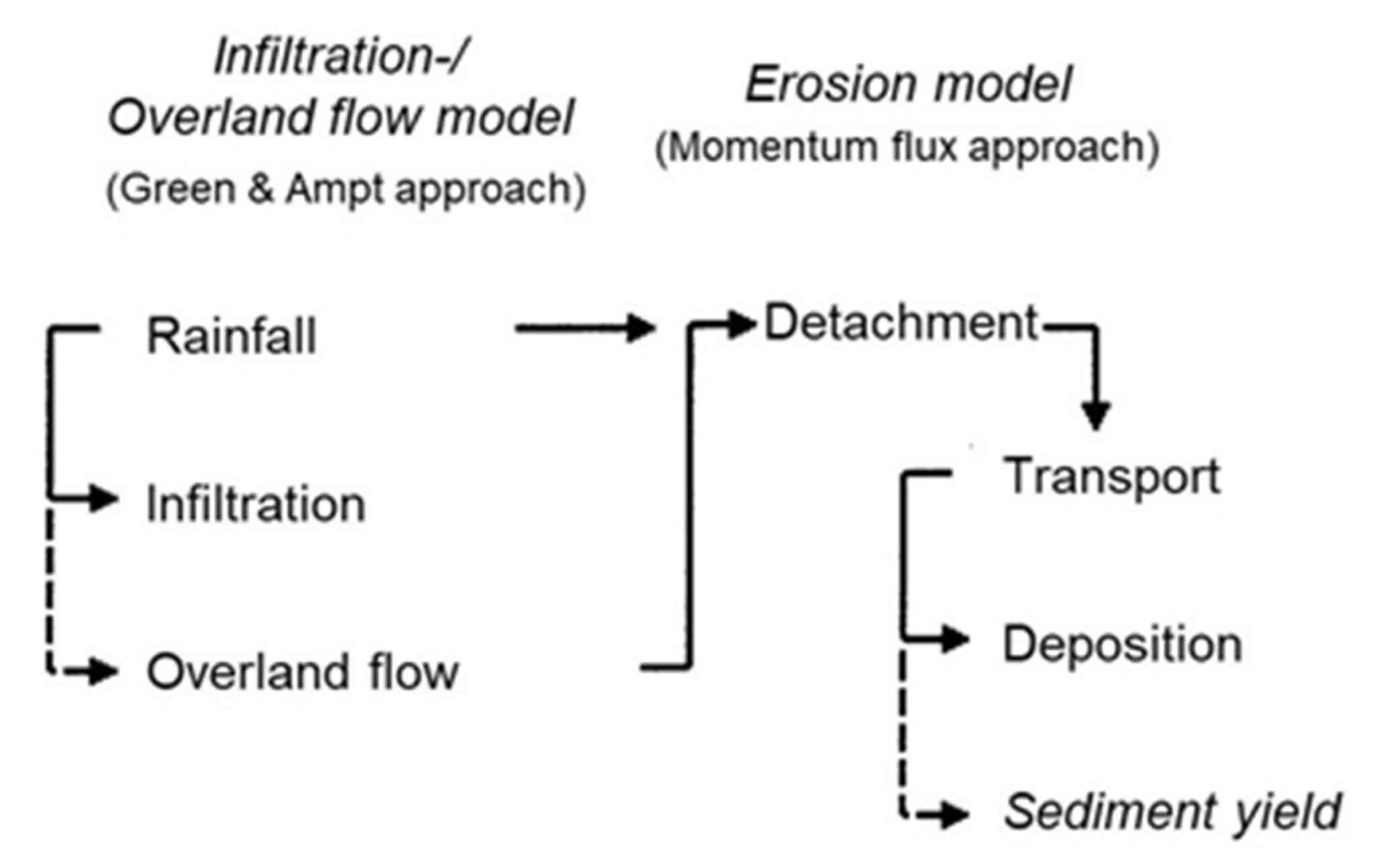
The structure of the EROSION-3D model consists of two main submodels, i.e., the infiltration and the erosion models (Figure 1). The calculations of the soil erosion are conducted by the erosion submodel, which considers the processes such as rainfall infiltration, generation of surface runoff, detachment of soil particles through the kinetic energy of raindrops and surface runoff or long-term modifications of the land surface relief due to soil erosion [27]. Because the EROSION-3D model is raster based, it requires a grid cell representation of a catchment.
The erosion submodel represents soil erosion processes in three steps, i.e., the detachment of soil particles from the impact of raindrops as well as their transport and deposition. The mathematical expression of the erosion submodule is based on the momentum flux approach [25], which involves an overland flow and is defined by the Equation:
where φqD is the momentum of the flux exerted by overland flow (N); q is the flow (m3/(m·s)); ρq is the fluid density (kg/m3); vq is the mean velocity of the flow according to Manning (m/s); and Δx is the length of a specified slope segment (m). Because the infiltration process is complicated, the mathematical description of the infiltration process is divided into the gravitational component i1 and the matrix component i2 as described below.
The gravitational component (i1) is defined by the gravitational potential as follows:
where i1 is the infiltration rate of the gravitational component (kg/(m2·s)); ks is the hydraulic conductivity of the transport zone ((kg·s)/m3); ∆ψg is the gravitational potential ((N·m)/kg); xf1 is the depth of the wetting front of the gravitational component (m); and g is the gravitational constant (m/s2).
The dynamic component of the matrix i2 is described by a function of the matrix potential Δψm:
where i2 is the infiltration rate of the matrix component (kg/(m2·s)); ks is the hydraulic conductivity of the transport zone ((kg·s)/m3); ∆ψm is the matrix potential ((N·m)/kg); and xf2(t) is the depth of the wetting front of the gravitational component (m) in time t.
The saturated hydraulic conductivity depends on the soil structure, soil texture, and the occurrence of macropores. For determining the saturated hydraulic conductivity, an empirical equation according to [28] is used:
where ks is the saturated hydraulic conductivity (kg·s/m3); ρb is the bulk density (kg/m³); T is the clay content (kg/kg); U is the silt content (kg/kg); D is the average particle size (m); δp is the standard deviation (-); and b is the local parameter (−).
2.2. Long-Term Simulation in the EROSION-3D Model
Although the EROSION-3D model has mainly been established as an event-based model, it contains the possibility of executing long-term simulations as an additional tool [29]. The long-term simulation submodel has a continuous character and can perform long-term simulations and run more calculations one after the other; after each event, the digital elevation model is adjusted to reflect the amount of erosion and deposition [25]. Long-term simulations can be performed in the following ways [30]:
- (1)
- The simulations are based on iterations where one or more events have recurred. How often single events or sequences of events are repeated is determined according to the iterative value.
- (2)
- A combination of individual single events is used to summarize the sequences of rainfall events. Based on this assumption, the model behaves like a continuous model and provides overall results.
- (3)
- A long-term simulation based on a continuous rainfall series consists of a chronological series of single rainstorms that occur within the period evaluated. Each rainfall event needs its own soil data set whose parameters account for the individual soil conditions and the stages of crop growth as of that date.
3. The Case Study
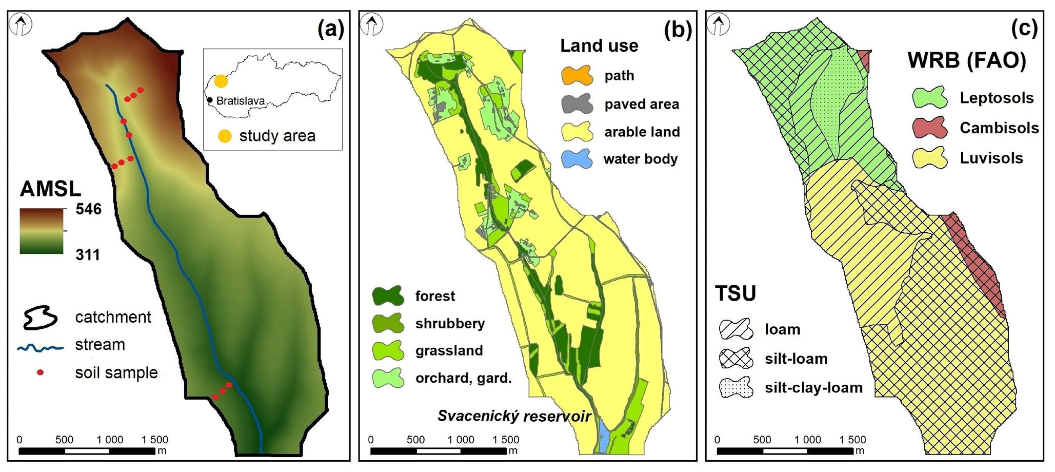
The Svacenický Creek catchment, which has a total area of 6.3 km2, is located in the Western Slovak Republic in the middle of the Myjava Hill Lands (Figure 2). The climate is continental, warm and moderately humid, with a mild winter and warm summer. The mean annual precipitation in the catchment is between 650 and 700 mm (1981–2015); the mean annual temperature is about 8.8 °C (1981–2013), as measured at the Myjava meteorological station. The elevation ranges from 311.4 m to 545.6 m a. s. l. The Svacenický Creek catchment is part of the flysch massif of the White Carpathians, and the dominant type of soil is Luvisols (68.0%), followed by Pararendzina (28.7%), and Cambisols (3.7%). The relief is composed of moderate slopes in the lower part of the catchment and narrow stream valleys with steep slopes in the upper part. The aerial-photograph from 2018 was used for creating of land use map and the arable land covers almost 66% of the catchment (Table 1).
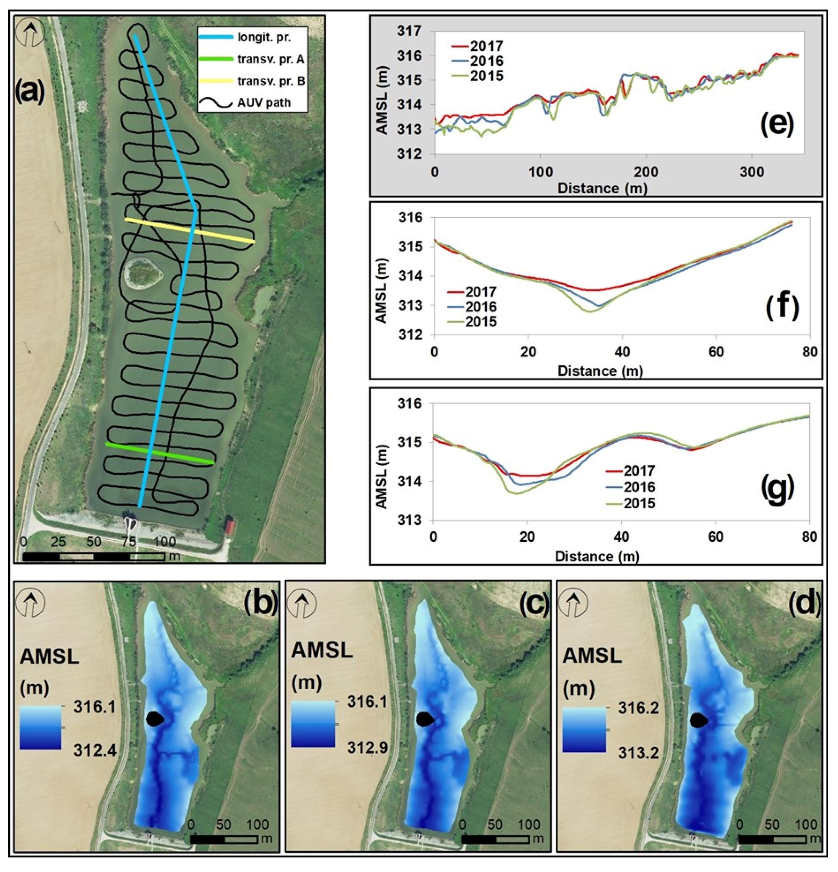
The Svacenický reservoir (Figure 2 and Figure 3) was constructed in 2010 at the bottom of the Svacenický Creek catchment as a flood-protection measure, and the permanent water level covers approximately 3 ha of the catchment. According to the project documentation [31], the height of the embankment dam is 10.25 m and the maximum retention capacity is 215,808 m3 with a maximum water level of 8.5 m. The planned minimum water level height is 4.4 m (316.4 m about mean sea level (AMSL)). The modelled retention capacity during a 100-year flood is 207,330 m3, with a peak discharge of 16.0 m3·s−1.
4. Data
An Autonomous Underwater Vehicle recorded the bathymetry in the Svacenický reservoir during field measurements carried out by the Slovak Academy of Science (SAS) in 2015 (22 September), 2016 (6 October) and 2017 (2 October). The EcoMapper is ideal for hydrographic spatial environmental monitoring in coastal and shallow-water applications. The speed of the AUV was 3.7 km/h and the sampling time interval was set at 1 s per sample. The total number of collected sample points is 2017 in 2015 and 2016, and 9211 sample points in 2017. The water level height was 4.45 m in 2015 and 2016, and 4.35 m in 2017. Figure 3 presents the results from the Digital Elevation Model (DEM) of the reservoir bottom with the 1 × 1 m spatial resolution. Post processing and data analysis were accomplished using Esri’s ArcGIS software (Jack Dangermond, Redlands, CA, United States) (ArcMap 10.7). The DEM of the Svacenický Creek reservoir was created by geostatistical analyst tool through the Topo to Raster. Topo to Raster provides the functionality of incorporating other types of geographic features, which can assist in the creation of a DEM. Finally, the input DEM of the Svacenický Creek catchment (in grid cell size 10 × 10 m) is provided by the Esprit spol. s.r.o. (cartographic company).
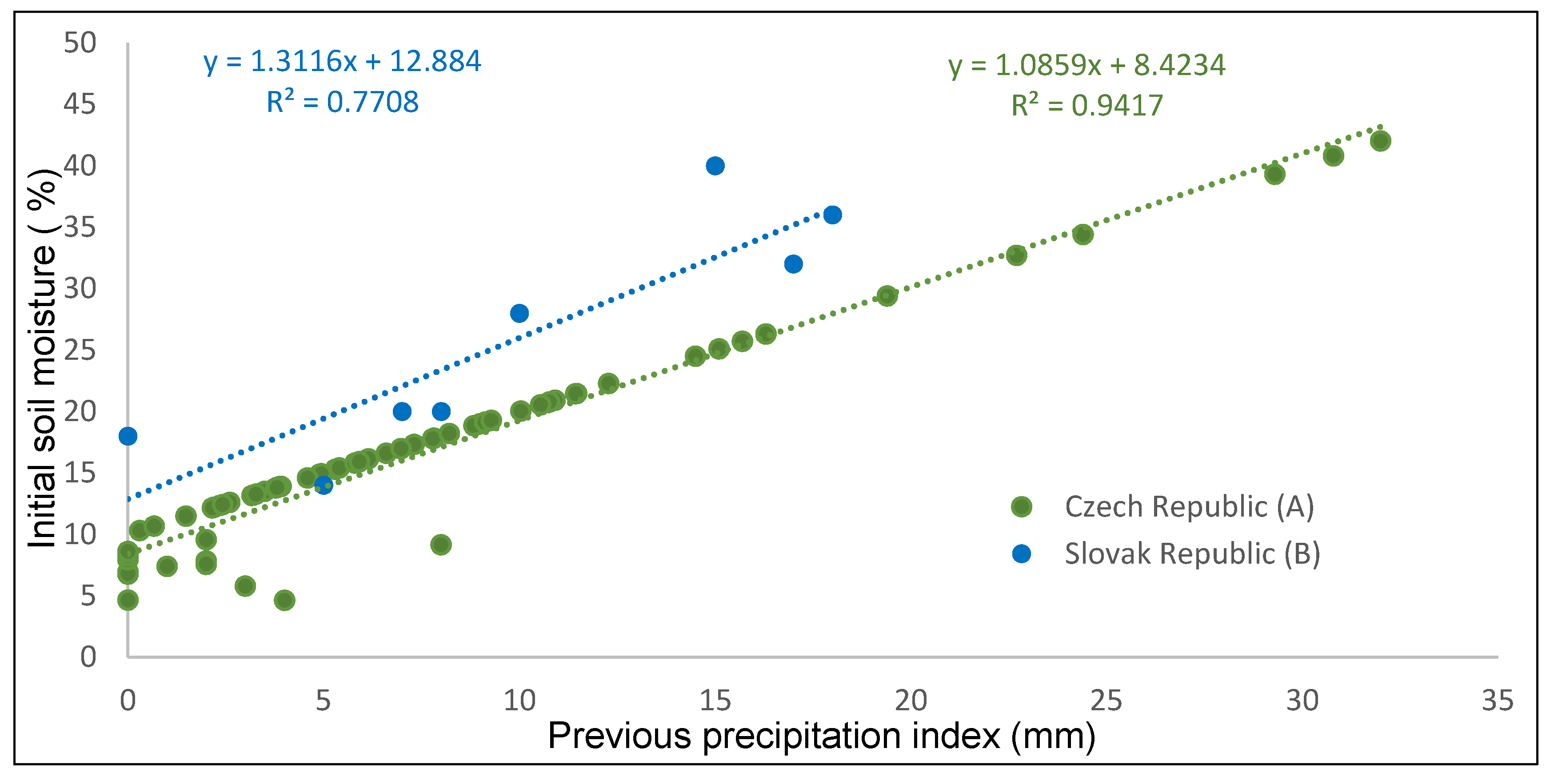
In comparison with other physically-based models like EUROSEM (The European Soil Erosion Model) [32], WEPP (The Water Erosion Prediction Project) [33], and LISEM (The Limburg Soil Erosion Model) [34], the EROSION-3D model requires fewer soil input parameters (Table 2). Some of the input soil data were acquired during field measurements, and the laboratory processing of eleven soil samples followed (Figure 2a, Table 3). Also, the initial soil moisture (one of the most unstable and changeable parameters) was determined based on the field measurements in the study area. The importance of this model input parameter is due to its correlation with the previous precipitation index (Figure 4). The previous precipitation index was estimated as the 5-days sum of antecedent precipitation amount before each simulated event. The functions are derived based on rainfall experiments with known rainfall intensities and durations. The rainfall experiments took place at experimental plots in Slovakia (the Myjava region) and the Czech Republic (the Plzen region) in cooperation with the Czech Technical University in Prague and with the Research Institute for Soil and Water Conservation. A graphical representation of the functions is shown in Figure 4 (A—data from the Czech Republic, B—data from the Slovak Republic). The soil input parameters from the Parameter Catalogue were estimated for the specific crop and its growth phase in different months within the year.
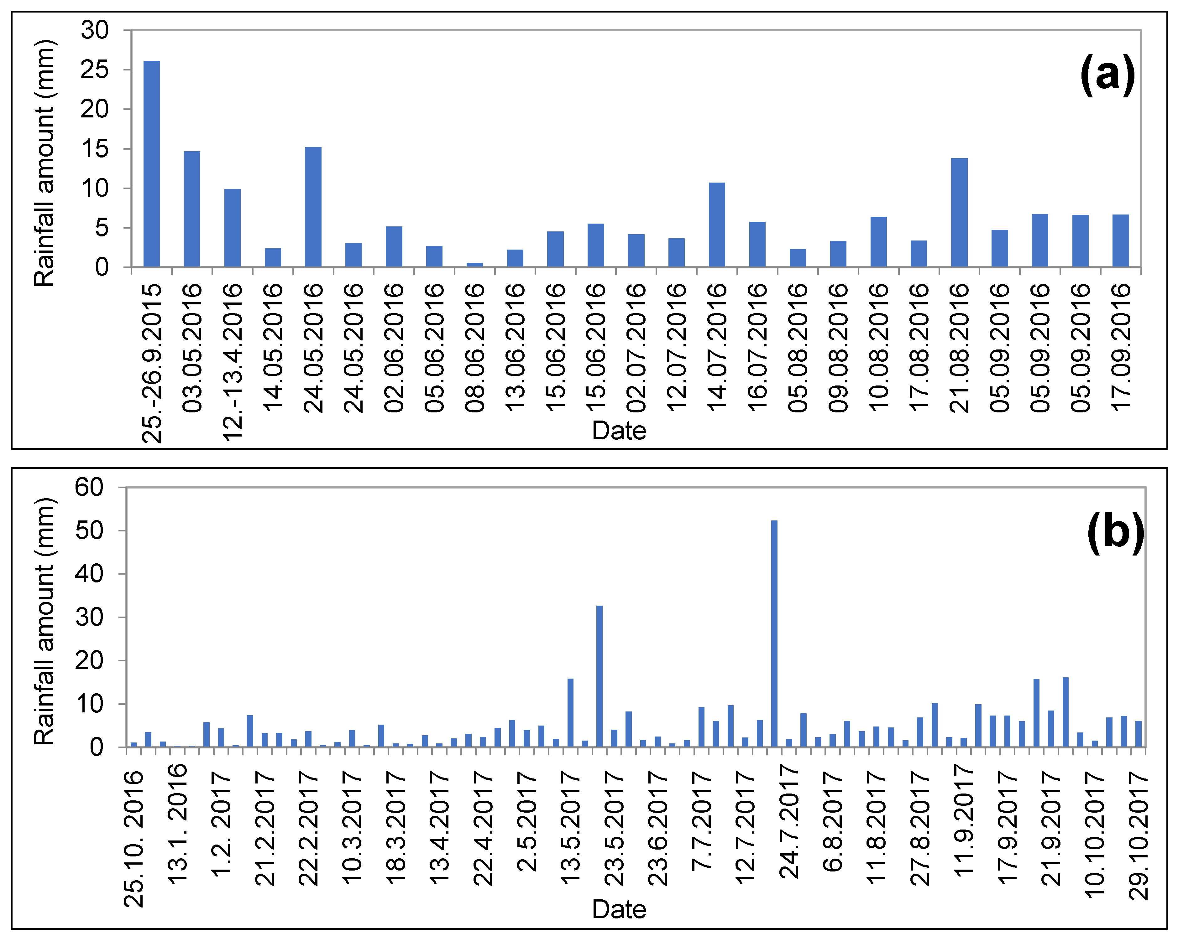
The rainfall data covers the time period investigated between September 2015 and October 2017. The rainfall events were used in the model calculations and the rainfall series consist of effective erosive events which occurred within the periods selected. Each rainfall event requires its own soil data set, whose parameters account for the current soil conditions and stages of crop growth of that date. The model runs were done for 95 rainfall events with specific rainfall intensities higher than 2 mm (for the model calculations, intensive rainfall events involved in soil erosion processes were selected). The summarized characteristics of the rainfall events selected are shown in Table 4. Figure 5 presents the occurrence of the selected rainfall events during the time period investigated.
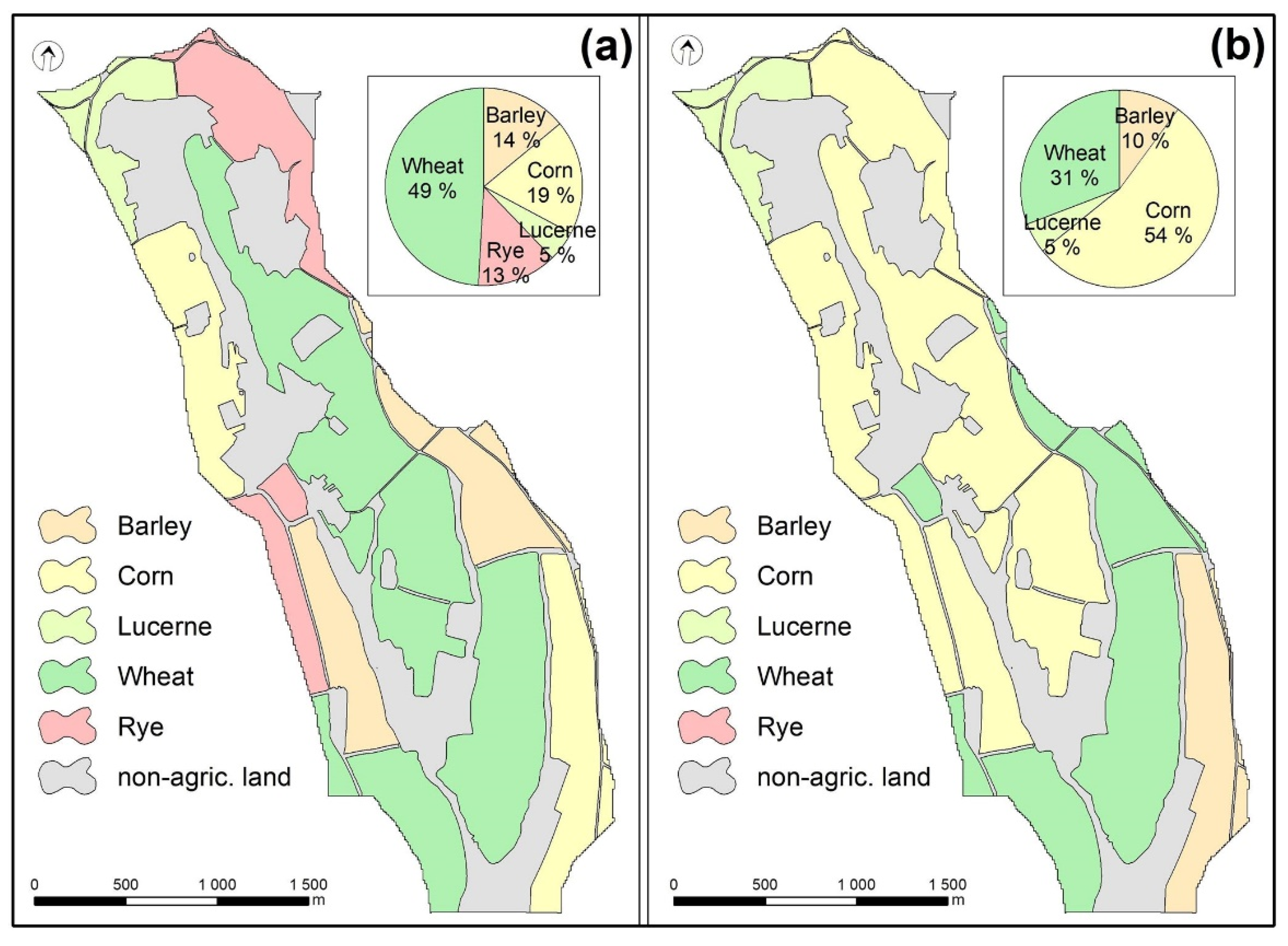
According to the documentation of the local farmers, 49% of the arable land (from September 2015 to October 2016) was covered by wheat, which was followed by corn (19%), barley (14%), rye (13%), and lucerne (5%). In the next time period (from October 2016 to October 2017), corn covered 54% of the arable land, which was followed by wheat (31%), barley (10%), and lucerne (5%). Figure 6 shows the spatial distribution of the crops in the study area from September 2015 to October 2016.
5. Results
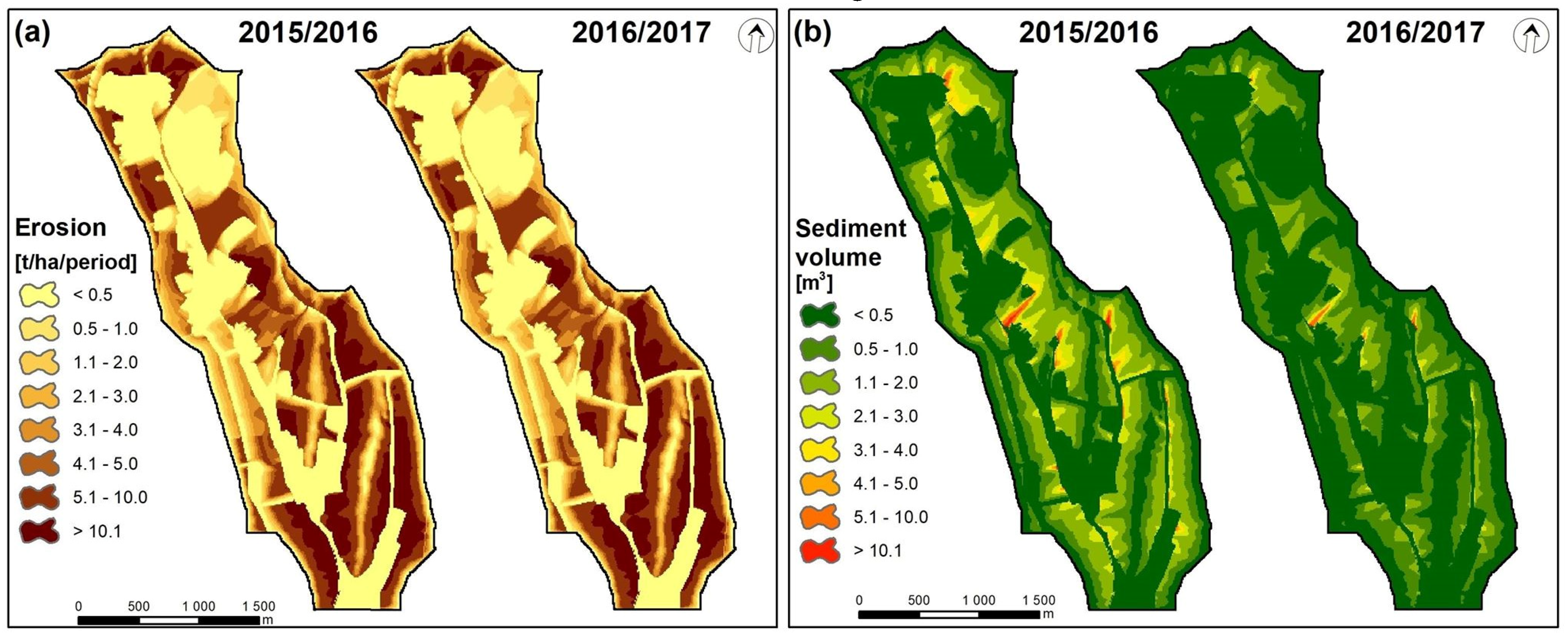
The arable land is influenced by the intensive erosion processes in the Svacenický Creek catchment. The most vulnerable areas are located at the bottom of the slopes and in the steepest parts of particular slopes (Figure 7a). The intensity of the erosion is often higher than 5.0 t/ha/yr. Together with inappropriate crop management (corn), these localities are exposed to extreme intensities of erosion processes (>10 t/ha/yr). Wide-row crops such as corn do not represent such a threat on short slopes as in the right part of the Svacenický Creek catchment. Nevertheless, narrow-row crops such as wheat or lucerne result in a lower rate of soil degradation (3–5 t/ha/yr). The intensities of the erosion look similar in both periods of time (Figure 7a). Nevertheless, there is a difference, which is more notable in the case of the volume of sediment (Figure 7b).
The intensive erosion processes are caused by intensive rainfall events. Table 5 presents the results for the rainfall-erosion events selected with a total rainfall amount higher than 12.5 mm [35,36,37]. In the first time period investigated (2015–2016), the rainfall-erosion events produced almost 23% of the eroded material compared to the total production of the time period in Table 6. On the other hand, only 2.4% of the sediments were produced by rainfall-erosion during the second time period investigated (2016–2017). The difference can be found in the total number of rainfall events, because the period 2016–2017 was richer in rainfall than the period 2015–2016, which made this period much drier and the soil more vulnerable to the erosion process.
The production of the eroded material is connected with areas of intensive erosion processes (Figure 7a). The total predicted sediment volume was 216.5 m3 in the period 2015–2016 and 375.8 m3 in the period 2016–2017. The higher amount of sediment in the period 2016–2017 correlates to the higher total number of rainfall events compared to the period 2015–2016. Comparing the predicted (modelled) and observed (bathymetric measured) sediment volume in the Svacenický reservoir, the EROSION-3D predicted a lower amount of sediments (Table 6). More specifically, the predicted volume of sediment (calculated for a function A) in the period 2015–2016 is 76% lower and 26% lower in the period 2016–2017 than the observed volume of sediment in the reservoir. Based on the function B, the production of sediment increased, and the modelled volume of sediment is even higher in the period 2016–2017 compared to the bathymetry. It must be noted that the actual measured volume of sediment was reduced by 56.5% because of the assumed water content in the reservoir sediment [38].
The eroded material reached the catchment outlet and the amount was measured by the AUV EcoMapper (YSI Company, Yellow Springs, OH, USA). The measured sediment volume was reduced by considering a sediment water content of 56.5% according to [38].
6. Discussion
The characteristics such as land use, and crop management (type of crop, crop rotation) belong to temporal dynamic features, while attributes such as slope morphology or type of soil represent relatively constant catchment characteristics [19]. The crop distribution with a higher amount of winter wheat pointed to a lower volume of sediments and generally less endangered soil [39]. The probable causes are the lower values for the parameters skin factor, surface roughness, and erosion resistance in comparison with corn. The higher amounts of the surface runoff (m3), the erosion and deposition rates (t/ha), and the volume of sediment (m3) in the Svacenický Creek catchment detected for the second period were the result of two main causes. The first one is the higher total number of rainfall events. The second cause lies in the crop management of the study area, where corn represents 54% of the arable land. The combinations of the effects of the management systems and rain conditions resulted in the higher amounts of erosion processes in the catchment. The type of crop has a great influence on the erosive process and soil losses [40]. There is a direct connection between the crop management system and soil losses; therefore, the crop management system is one of the main factors affecting soil erosion by water [40]. Appropriate land management can significantly help reduce erosion processes [41,42,43]. In the case of model parameters, the biggest influence on runoff and erosion processes has bulk density, soil moisture and skin factor. The skin factor is the parameter used to reduce the prediction error resulting from the simplified assumptions of the model because the EROSION-3D model considers simplifications of homogenous soil matrix, but the process of infiltration is influenced by many different factors, i.e., soil compaction, soil crusting, surface soil pores, biological activity due to rodent burrows or worm and it is necessary to include correcting parameter.
Although erosion resistance and hydraulic roughness are considered as important factors, it has been found that they do not affect model results to a significant extent. However, the general trend of decreasing resistance of erosion with increasing erosion intensity has been confirmed by experimental results [44,45].
The results also pointed to the importance of rainfall-erosion events that are able to result in high erosion of soil [46]. In this case, the role of such events could increase in the future because of the predicted increase in extreme rainfall events due to climate change [4,46,47,48,49,50]. According to the Slovak Hydrometeorological Institute, the number of rainfall events with durations of 5 to 240 min has been increasing during the last decade, while rainfall-erosion events occur 2.5 to 4.7 times per year; this amount is expected to increase in the future, especially during the spring and summer months [51,52].
When testing the application of the EROSION-3D model, some difficulties were found during the appropriate determination of the input parameters and when verifying the model results through the actual measured data. A model dependability heavily depends on its calibration [53] and the testing of a physically-based erosion model is considered as a necessary part of any scientific work in order to develop an understanding of what the model will demonstrate [54].
Due to the testing process, the strengths and weaknesses of a model can be discovered. According to [55], long-term results are generally simulated in the best possible way. Here, the results presented pointed at a notable difference between the modelled and observed sediment yields, which indicates the difficulty posed by the model simplification of the natural phenomenon of erosion [18].
As it is mentioned in [56], mathematical simulation models consist of three sub-models: (a) Rainfall-runoff submodel, (b) a soil erosion sub-model and (c) a stream sediment transport sub-model. All three sub-models should be considered, but in this case, it was not done, because relevant data for stream sediment transport sub-model was not possible to obtain. In spite of a fact that small streams exist in the polder basin, significant flow occurs only in case of intense precipitation. This fact largely limits the acquirement and measurement of the relevant data needed to calculate the flow of streambed erosion. In addition to that, it can be seen (Figure 2a), that majority of these small streams flow in low slope area, so flow velocity is also low and so, frame velocity is a weak one as well. So, for this reason, we assume this type of erosion has not to be taken into account. Besides all, the used simulation model cannot simulate it as well.
However, this part of the available sediments in the catchment should be taken into account [56], but because of the conditions mentioned above, there was not done. On the other hand, during the three-years monitoring time there was found depositions of sediment in one inlet part of the reservoir (the longest contributing creek), that confirm flow stream erosion, but their volume is not significant. From all of those, it can be supposed that omission of streambed erosion could be a part of differences between calculated and measured /observed sediment volume data.
As is mentioned, based on the field measurements of the bottom bathymetry which started in 2015, the current status of the clogging of the reservoir was evaluated. The results confirmed our theories about the on-going sedimentation processes in the Svacenicky Creek reservoir. According to the analysis, we determined that during the years 2012–2019, over 10.4285 m3 of sediment on the area of the Svacenicky Creek catchment have accumulated and the polder volume capacity has decreased 6%. The average sediment transport during the years was estimated to be 1400 t/year. The sediment transport has lowered since 2016, which can be e.g., due to lower precipitations as also flood protection measures adopted in this area. According to Table 6, the lifetime of the reservoir varies between 303.7 years for observed sedimentation, 315.0 years for predicted sedimentation B and 728.7 years for sedimentation A.
Possible sources of errors in the predicted sediment volume by the EROSION-3D model can mostly be associated with the model parameters, values of the initial soil moisture before each simulated event, and the grid size of the catchment area. The parameters of the EROSION-3D model as the resistance to erosion, surface roughness, and skin factor were chosen from the Parameter Catalogue for EROSION-3D, which contains their tabularized values by the type of soil, land use and the specific crop and its growth phase in different months within the year. Because of the attempt to continual modelling based on the modelling of a sequence of individual rainfall-erosion events, it was not possible to calibrate these parameters for each event. For the continual modelling, the crucial input parameters were the values of initial soil moisture before each simulated rainfall-erosion event. The values of initial soil moisture were estimated from the relationships between the soil moisture and the previous precipitation index, developed experimentally for the Plzen region in the Czech Republic (Figure 4, function A) and for the experimental plots in the Myjava region in Slovakia (Figure 4, function B). The data of initial soil moisture estimated from the function developed for the Myjava region in Slovakia, which is more representative for the case study area, improved the predictive sediment volumes in comparison with the measured sediment volumes—the relative error decreased to 40% for the period 2015–2016 and 30% for the period 2016–2017. On the other hand, the function B was developed only from seven pairs of experimental data, and we suppose that the extension of the data and improvement of this function would improve the performance of the model.
Also, the use of bathymetry to estimate trapped sediment in a reservoir brings out other uncertainties. According to [23], several problems with this method can be observed, e.g., the unknown effectiveness of the reservoir, the importance of a detailed analysis of the sediment cores; the precise location of sources of the sediment; the size of the reservoir and related discharges; and depreciation of the organic fraction of the sediment due to the measurements. Nevertheless, the bathymetric method is arguably the best way to determine the volume of sediment and can be carried out by several approaches [23,24,57]. The use of the autonomous underwater vehicle (AUV) to investigate the temporal evolution of changes in the bottom of the reservoir through the DEM was approved in this paper.
7. Conclusions
The physically-based EROSION-3D model was applied to simulate the runoff-erosion processes in the Slovak catchment. The model helps to identify the most sensitive erosion and deposition zones within a catchment. The long-term simulations were done for two periods (2015–2016 and 2016–2017), which were evaluated according to the time of the bathymetric measurements conducted. The results of the model pointed to an underestimation of the actual processes. The initial soil moisture plays an important role through all the input parameters of the EROSION-3D model. Finally, the rainfall- erosion events were able to erode and produce a significant part of the sediments, especially during a drier year or season.
Author Contributions
Conceptualization, Z.N. and D.H.; methodology, Z.N., D.H., S.K. and K.H.; software, Z.N., V.S. and Y.V.; validation, Z.N. and D.H.; formal analysis, Z.N. and D.H.; investigation, Z.N., D.H., V.S. and Y.V.; writing—original draft preparation, Z.N., D.H and M.Š.M.; writing—review and editing, S.K., K.H. and M.Š.M.; visualization, D.H. All authors have read and agreed to the published version of the manuscript.
Funding
This project was funded by Contracts No. APVV-15-0497 and VEGA Grant Agency No. 1/0632/19. This work was supported by the Specific Research project at Masaryk University (MUNI/A/1356/2019), the Slovak Research and Development Agency under Contracts No. APVV-15-0497, APVV-18-0347 and APVV-18-0205, the VEGA Grant Agency No. 1/0632/19 and No. 2/0025/19. The authors thank the agency for its research support
Conflicts of Interest
The authors declare no conflict of interest.
References
- Rawat, P.K.; Tiwari, P.C.; Pant, C.C.; Sharama, A.K.; Pant, P.D. Modelling of stream run-off and sediment output for erosion hazard assessment in Lesser Himalaya: Need for sustainable land use plan using remote sensing and GIS: A case study. Nat. Hazards 2011, 59, 1277–1297. [Google Scholar] [CrossRef]
- Markantonis, V.; Meyer, V.; Schwarze, R. Valuating the intangible effects of natural hazards—Review and analysis of the costing methods. Nat. Hazards Earth Syst. Sci. 2012, 12, 1633–1640. [Google Scholar] [CrossRef]
- Wainwright, J.; Parsons, A.J.; Michaelides, K.; Powell, D.M.; Brazier, R. Linking Short- and Long-Term Soil—Erosion Modelling. In Long Term Hillslope and Fluvial System Modelling, 1st ed.; Lang, A., Dikau, R., Eds.; Springer: Berlin/Heidelberg, Germany, 2003; pp. 37–51. [Google Scholar]
- Hlavčová, K.; Kohnová, S.; Borga, M.; Horvát, O.; Šťastný, P.; Pekárová, P.; Majerčáková, O.; Danáčová, Z. Post-event analysis and flash flood hydrology in Slovakia. J. Hydr. Hydrom. 2016, 64, 304–315. [Google Scholar] [CrossRef] [Green Version]
- Renfro, W.G. Use of erosion equation and sediment delivery ratios for predicting sediment yield. In Present and Prospective Technology for Predicting Sediment Yields and Sources, 1st ed.; US Department of Agriculture Publication ARS-S-40: Washington, DC, USA, 2018; pp. 33–45. [Google Scholar]
- Kirkby, M.J.; Morgan, R.P.C. Soil Erosion, 1st ed.; John Wiley and Sons: Chichester, UK, 1980; p. 306. [Google Scholar] [CrossRef]
- Walling, D.E. The sediment delivery problem. J. Hydrol. 1983, 65, 209–237. [Google Scholar] [CrossRef]
- Richards, K. Sediment delivery and drainage network. In Channel Network Hydrology, 1st ed.; Beven, K., Ed.; Wiley: New York, NY, USA, 1993; Volume 1, pp. 221–254. [Google Scholar]
- Atkinson, E. Methods for assessing sediment delivery in river systems. Hydrol. Sci. J. 1995, 40, 273–280. [Google Scholar] [CrossRef] [Green Version]
- Wischmeier, W.H.; Smith, H. Predicting Rainfall Erosion Losses—A Guide to Conservation Planning, 1st ed.; U.S. Dep. of Agriculture: Washington, DC, USA, 1978; p. 85.
- Nearing, M.A.; Lane, L.J.; Lopes, V.L. Modeling Soil Erosion. In Soil Erosion Research Methods, 2nd ed.; Lal, R., Ed.; Routledge: New York, NY, USA, 1994; p. 127. [Google Scholar]
- Kandel, D.D.; Western, A.W.; Grayson, R.B.; Turral, H.N. Process parameterization and temporal scaling in surface runoff and erosion modelling. Hydrol. Process. 2004, 18, 1423–1446. [Google Scholar] [CrossRef]
- Merritt, W.S.; Letcher, R.A.; Jakeman, A.J. A review of erosion and sediment transport models. Environ. Mod. Soft. 2003, 18, 761–799. [Google Scholar] [CrossRef]
- Kwong, F.A.L. Quantifying Soil Erosion for the Shihmen Reservoir Watershed, Taiwan. Agric. Sys. 1994, 45, 105–116. [Google Scholar] [CrossRef]
- Pandey, A.; Himanshu, S.K.; Mishra, S.K.; Singh, V.P. Physically based soil erosion and sediment yield models revisited. Catena 2016, 147, 595–620. [Google Scholar] [CrossRef]
- Hajigholizadeh, M.M.; Hector, A.F. Erosion and Sediment Transport Modelling in Shallow Waters: A Review on Approaches, Models and Applications. Int. J. Environ. Res. Public Health 2018, 15, 518. [Google Scholar] [CrossRef] [Green Version]
- Jakeman, A.J.; Green, T.R.; Beavis, S.G.; Zhang, L.; Dietrich, C.R.; Crapper, P.F. Modelling upland and instream erosion, sediment and phosphorus transport in a large catchment. Hydrol. Process. 1999, 13, 745–752. [Google Scholar] [CrossRef]
- Kuznetsov, M.S.; Gendugov, V.M.; Khalilov, M.S.; Ivanuta, A.A. An equation of soil detachment by flow. Soil Tillage Res. 1998, 46, 97–102. [Google Scholar] [CrossRef]
- Wei, H.; Nearing, M.A.; Stone, J.J.; Guertin, D.P.; Spaeth, K.E.; Pierson, F.B.; Nichols, M.H.; Moffet, C.A. A New Splash and Sheet Erosion Equation for Rangelands. Soil Sci. Soc. Am. J. 2009, 73, 1386–1392. [Google Scholar] [CrossRef]
- Iglesias, I.; Avilez-Valente, P.; Bio, A.; Bastos, L. Modelling the Main Hydrodynamic Patterns in Shallow Water Estuaries: The Minho Case Study. Water 2019, 11, 1040. [Google Scholar] [CrossRef] [Green Version]
- Marttila, H.; Klöve, B. Dynamics of erosion and suspended sediment transport from drained peatland forestry. J. Hydrol. 2010, 388, 414–425. [Google Scholar] [CrossRef]
- Ayele, G.T.; Teshale, E.Z.; Yu, B.; Rutherfurd, I.D.; Jeong, J. Streamflow and Sediment Yield Prediction for Watershed Prioritization in the Upper Blue Nile River Basin, Ethiopia. Water 2017, 10, 782. [Google Scholar] [CrossRef] [Green Version]
- García-Ruiz, J.M.; Beguería, S.; Nadal-Romero, E.; González-Hidalgo, J.C.; Lana-Renault, N.; Sanjuán, Y. A meta-analysis of soil erosion rates across the world. Geomorphology 2015, 239, 160–173. [Google Scholar] [CrossRef] [Green Version]
- Boyle, J.F.; Plater, A.J.; Mayers, C.; Turner, S.D.; Stroud, R.W.; Weber, J.E. Land use, soil erosion, and sediment yield at Pinto Lake, California: Comparison of a simplified USLE model with the lake sediment record. J. Paleolimnol. 2011, 45, 199–212. [Google Scholar] [CrossRef]
- Schmidt, J. A mathematical model to simulate rainfall erosion. Catena 1991, 19, 101–109. [Google Scholar]
- Green, W.H.; Ampt, G. Studies of soil physics: The flow of air and water through soils. J. Agric. Sci. 1911, 4, 1–24. [Google Scholar]
- Von Werner, M. Erosion-3D: User Manual, version. 3.1.1; Michael von Werner Berlin: Berlin, Germany, 2006; p. 54. [Google Scholar]
- Campbell, G.S. Soil physics with basic: Transport models for soil-plant systems. DEV. Soil Sci. 1985, 14, 252–254. [Google Scholar]
- Von Werner, M. Erosion-3D Version 3.0 User Manual—Samples. 2003; GeoGnostics Software: Berlin, Germany, 2003; p. 34. [Google Scholar]
- Schmidt, J. Development and Application of a Physically Established Simulation Model for the Erosion of Agricultural Areas; Institute of Geographic Sciences: Berlin, Germany, 1996; p. 148. [Google Scholar]
- VODOTIKA. Polder Svacenický Creek. Bratislava, 10-01-2008; Project documentation; Vodotika: Bratislava, Slovak Republic, 2008; p. 35. [Google Scholar]
- Morgan, R.; Quinton, J.; Smith, R.; Govers, G.; Poesen, J.; Auerswald, K.; Chisci, C.; Torri, D.; Styczen, M.E. The European soil erosion model (EUROSEM)—A process-based approach for predicting sediment transport from fields and small catchments. Earth Surf. Proc. Land. 1998, 23, 527–544. [Google Scholar] [CrossRef]
- Laflen, J.M.; Elliot, W.J.; Flanagan, D.C.; Meyer, C.R.; Nearing, M.A. WEPP-predicting water erosion using a process-based model. J. Soil Water Conserv. 1997, 52, 96–102. [Google Scholar]
- De Roo, A.P.J.; Wesseling, C.G.; Ritsema, C.J. LISEM: A single event physically based hydrological and soil erosion model for drainage basins. I: Theory, input and output. Hydrol. Process. 1996, 10, 1107–1117. [Google Scholar] [CrossRef]
- Stocking, M.A.; Elwell, H.A. Rainfall erosivity over Rhodesia. Trans. Inst. Brit. Geogr. 1976, 1, 231–245. [Google Scholar] [CrossRef]
- Pasák, V. Soil Protection against Erosion, 1st ed.; State Agricultural Publishing House Prague: Prague, Czech, 1984; p. 164. [Google Scholar]
- Brychta, J.; Janeček, M. Determination of erosion rainfall criteria based on natural rainfall measurement and its impact on spatial distribution of rainfall erosivity in the Czech Republic. Soil Water Res. 2019, 14, 153–162. [Google Scholar] [CrossRef]
- Hucko, P.; Šumná, J. Verification of the System of Sediment Disposal from Water Management Reservoirs, 1th ed.; VÚVH: Bratislava, Slovak, 2003. [Google Scholar]
- Schindewolf, M.; Bornkampf, C.; von Werner, M.; Schmidt, J. Simulation of Reservoir Siltation with a Process-based Soil Loss and Deposition Model. In Effects of Sediment Transport on Hydraulic Structures; Vlassias, H., Ed.; Democritus University of Thrace: Xanthi, Greece, 2015; pp. 41–57. [Google Scholar] [CrossRef] [Green Version]
- Carvalho, D.F.; Eduardo, E.N.; de Almeida, W.S.; Santos, L.A.F.; Sobrinho, T.A. Water erosion and soil water infiltration in different stages of corn development and tillage systems. Rev. Bras. Eng. Agríc. Ambient. Agric. 2015, 19, 1072–1078. [Google Scholar] [CrossRef] [Green Version]
- Panagos, P.; Borelli, P.; Meusburger, K.; Alewell, C.; Lugato, E.; Montanarella, L. Estimating the soil erosion cover-management factor at the European scale. Land Use Policy 2015, 48, 38–50. [Google Scholar] [CrossRef]
- Bo, M.; Xiaoling, Y.; Fan, M.; Zhanbin, L.; Faqi, W. Effects of Crop Canopies on Rain Splash Detachment. PLoS ONE 2014, 9, 10. [Google Scholar] [CrossRef]
- Hugo, V.; Zuazo, D.; Rocío, C.; Pleguezuelo, R. Soil-erosion and runoff prevention by plant covers. A review. Agric. Sustain. Dev. 2008, 1, 65–86. [Google Scholar] [CrossRef] [Green Version]
- Ebabu, K.; Tsunekawa, A.; Haregeweyn, N.; Adgo, E.; Meshesha, D.T.; Aklog, D.; Masunaga, T.; Tsubo, M.; Sultan, D.; Fenta, A.A.; et al. Effects of land use and sustainable land management practices on runoff and soil loss in the Upper Blue Nile basin. Sci. Total Environ. 2019, 648, 1462–1475. [Google Scholar] [CrossRef] [PubMed]
- Knapen, A.; Poesen, J.; De Baets, S. Seasonal variations in soil erosion resistance during concentrated flow for a loess-derived soil under two contrasting tillage practices. Soil Tillage Res. 2007, 94, 425–440. [Google Scholar] [CrossRef]
- Uhrová, J.; Bachan, R.; Štěpánková, P. Determination of soil loss from erosion rills by method of digital photogrammetry and method of volumetric quantification. VTEI 2018, 6, 35–38. [Google Scholar]
- Uhrová, J.; Štěpánková, P.; Osičkovám, K. Complex system of natural water retention measures against erosion and flash floods. VTEI 2016, 4, 13–19. [Google Scholar]
- Michael, A. Anwendung des Physikalisch Begründeten Erosionsprognosemodells EROSION 2D/3D—Empirische Ansätze zur Ableitung der Modellparameter. Ph.D. Thesis, Technische Universität Bergakademie Freiberg, Freiberg, Germany, 2000. [Google Scholar]
- Zolina, O.; Simmer, C.; Kapala, A.; Shabanov, P.; Becker, P.; Mächel, H.; Gulev, S.; Groisman, P. Precipitation Variability and Extremes in Central Europe: New View from STAMMEX Results. Bull. Am. Met. Soc. 2014, 99, 995–1002. [Google Scholar] [CrossRef] [Green Version]
- Dolák, L.; Řezníčková, L.; Dobrovolný, P.; Štěpánek, P.; Zahradníček, P. Extreme precipitation totals under present and future climatic conditions according to regional climate models. In Climate Change Adaptation Pathways from Molecules to Society, 1st ed.; Vačkář, D., Ed.; Global Change Research Institute, Czech Academy of Sciences: Brno, Czech, 2017; pp. 27–37. [Google Scholar]
- Trnka, M.; Brázdil, R.; Vizina, A.; Dobrovolný, P.; Mikšovský, J.; Štěpánek, P.; Hlavinka, P.; Řezníčková, L.; Žalud, Z. Droughts and Drought Management in the Czech Republic in a Changing Climate. In Drought and Water Crises: Integrating Science, Management, and Policy, 1st ed.; Wilhite, D.A., Ed.; CRC Press, Taylor & Francis: Boca Raton, FL, USA, 2017; pp. 461–480. [Google Scholar]
- Slovak Hydrometeorological Institute (Increase in the Extremes of Total Rainfall Events in Slovakia). Available online: http://www.shmu.sk/sk/?page=2049&id=965 (accessed on 20 March 2019).
- Acuña, G.J.; Ávila, H.; Fausto, A.C. River Model Calibration Based on Design of Experiments Theory. A Case Study: Meta River, Colombia. Water 2019, 11, 1382. [Google Scholar] [CrossRef] [Green Version]
- Quinton, J. The Validation of Physically-based Erosion Models with Particular Reference to EUROSEM. Ph.D. Thesis, Cranfield University, Wharley End, UK, 1994. [Google Scholar]
- Favis-Mortlock, D.; Boardman, J.; Bell, M. Modelling long-term anthropogenic erosion of a loess cover: South Downs, UK. Holocene 1997, 7, 79. [Google Scholar] [CrossRef]
- Hrissanthou, V. Computation of Lake or Reservoir Sedimentation in Terms of Soil Erosion, In Sediment Transport in Aquatic Environments, 3rd ed.; Manning, A.J., Ed.; IntechOpen: London, UK, 2011; pp. 233–262. [Google Scholar] [CrossRef] [Green Version]
- Zhao, G.; Mu, X.; Jiao, J.; Gao, P.; Sun, W.; Li, E.; Wei, Y.; Huang, J. Assessing response of sediment load variation to climate change and human activities with six different approaches. Sci. Total Environ. 2018, 639, 773–784. [Google Scholar] [CrossRef]
Figure 1.
The EROSION-3D model structure [24].
Figure 1.
The EROSION-3D model structure [24].

Figure 2.
The characteristics of the Svacenický Creek catchment study area: (a) Relief, soil samples and location in the Slovak Republic; (b) land use; (c) textural soil unit (TSU) and World Reference Base (WRB(FAO)).
Figure 2.
The characteristics of the Svacenický Creek catchment study area: (a) Relief, soil samples and location in the Slovak Republic; (b) land use; (c) textural soil unit (TSU) and World Reference Base (WRB(FAO)).

Figure 3.
The Svacenický reservoir: (a) The autonomous underwater vehicle (AUV) EcoMapper path and longitudinal/transversal profiles; DEM of the reservoir in (b) 2015, (c) 2016, and (d) 2017; Graphs of the bottom’s development—(e) longitudinal profile, (f) transversal profile A, (g) transversal profile B.

Figure 4.
The functions (dependence) between the initial soil moisture and previous precipitation index determined according to the field measurements in the Slovak and Czech Republics.
Figure 4.
The functions (dependence) between the initial soil moisture and previous precipitation index determined according to the field measurements in the Slovak and Czech Republics.

Figure 5.
Total rainfall amounts and date of occurrence of selected rainfall events during the two time periods: (a) September 2015–October 2016; (b) October 2016–October 2017.
Figure 5.
Total rainfall amounts and date of occurrence of selected rainfall events during the two time periods: (a) September 2015–October 2016; (b) October 2016–October 2017.

Figure 6.
Annual crop distribution in the study area: (a) 2015–2016; (b) 2016–2017.

Figure 7.
Results from the EROSION-3D model (calculated for a function A): (a) Erosion intensity; (b) Volume of sediment.
Figure 7.
Results from the EROSION-3D model (calculated for a function A): (a) Erosion intensity; (b) Volume of sediment.


Table 1.
The land use categories in the study area.
| Land Use Category | Total | Path | Paved Area | Arable Land | Water Body | Forest | Shrubbery | Grassland | Orchard, Garden |
|---|---|---|---|---|---|---|---|---|---|
| Area (km2) | 6.26 | 0.03 | 0.11 | 4.11 | 0.49 | 0.55 | 0.06 | 0.54 | 0.37 |
| Area (%) | 100 | 0.5 | 1.8 | 65.7 | 7.8 | 8.8 | 1.0 | 8.6 | 5.9 |
Table 2.
The input soil parameters required by the EROSION-3D model.
| Input Parameter | Unit | Data Source |
|---|---|---|
| Altitude (DEM) | (m) | Esprit, s. r. o. |
| Rainfall intensity per time step | (mm/min) | Slovak Hydrometeorological Institute |
| Bulk density | (kg/m3) | Field measurement |
| Organic carbon content | (%) | Field measurement |
| Grain size distribution | (%) | Field measurement |
| Skin factor | (−) | Parameter Catalogue |
| Surface roughness | (s/m1/3) | Parameter Catalogue |
| Initial soil moisture | (%) | Field measurement |
| Erosion resistance | (N/m2) | Parameter Catalogue |
Table 3.
The soil characteristics in the study area.
| Soil ID | Soil Particle Size (%) | Organic Carbon Content (%) | Bulk Density (g/cm3) | ||
|---|---|---|---|---|---|
| Sand | Silt | Clay | |||
| 1 | 15.9 | 55.7 | 5.1 | 9.5 | 1.070 |
| 2 | 19.4 | 53.1 | 2.8 | 12.5 | 1.161 |
| 3 | 19.1 | 41.4 | 3.6 | 11.8 | 1.032 |
| 4 | 8.4 | 73.5 | 7.2 | 8.8 | 1.097 |
| 5 | 7.8 | 76.5 | 6.3 | 9.4 | 1.011 |
| 6 | 9.1 | 71.9 | 7.0 | 9.2 | 1.466 |
| 7 | 9.8 | 68.3 | 7.2 | 12.1 | 1.334 |
| 8 | 3.6 | 69.5 | 12.1 | 15.1 | 0.890 |
| 9 | 9.8 | 68.3 | 7.2 | 12.1 | 1.334 |
| 10 | 8.9 | 70.4 | 7.2 | 12.8 | 1.048 |
| 11 | 7.9 | 75.0 | 6.5 | 10.9 | 0.982 |
Table 4.
Characteristics (minimum, maximum and mean value ) of the selected 95 rainfall events between September 2015 and October 2017.
Table 4.
Characteristics (minimum, maximum and mean value ) of the selected 95 rainfall events between September 2015 and October 2017.
| Time Period | Duration (min) | Rainfall Amount (mm) | Rainfall Intensity (mm/min) |
|---|---|---|---|
| 2015–2016 | 1–1041 ( 141) | 0.57–26.11 ( 6.63) | 0.02–0.57 ( 0.12) |
| 2016–2017 | 10–504 (86) | 0.28–52.30 (5.59) | 0.02–0.71 ( 0.10) |
Table 5.
Results from the EROSION-3D model calculated for the erosion-rainfall events (total rainfall amount >12.5 mm; [35,36,37] and function A.
| Date | Duration (min) | Rainfall Amount (mm) | Rainfall Intensity (mm/min) | Surface Runoff (m3) | Erosion/Deposition Rate (t/ha) | Sediment Volume (m3) |
|---|---|---|---|---|---|---|
| 25–26 September 2015 | 1041 | 26.11 | 0.03 | 10.20 | 2.75 | 12.27 |
| 3 May 2016 | 206 | 14.66 | 0.07 | 6.25 | 0.35 | 15.66 |
| 24 May 2016 | 161 | 15.22 | 0.09 | 6.23 | 0.00 | 13.54 |
| 21 August 2016 | 79 | 13.8 | 0.18 | 4.33 | 0.18 | 7.60 |
| Total Sediment Production: | 49.07 | |||||
| 13 May 2017 | 51 | 15.8 | 0.31 | 4.20 | 1.36 | 1.19 |
| 23 May 2017 | 58 | 32.67 | 0.56 | 10.20 | 2.37 | 1.30 |
| 22 July 2017 | 74 | 52.3 | 0.71 | 22.30 | 2.36 | 1.41 |
| 21 September 2017 | 504 | 15.74 | 0.03 | 10.60 | 2.57 | 3.87 |
| 3 October 2017 | 226 | 16.07 | 0.07 | 0.50 | 0.21 | 1.23 |
| Total Sediment Production: | 9.00 | |||||
Table 6.
Comparison between the bathymetric measured data and modelled data of the sediment budget in the Svacenický reservoir (2015–2017).
Table 6.
Comparison between the bathymetric measured data and modelled data of the sediment budget in the Svacenický reservoir (2015–2017).
| Time Period | Predicted Sediment Volume (1) (m3) | Predicted Sediment Volume (2) (m3) | Observed Sediment Volume (m3) | Relative Error (%) | |
|---|---|---|---|---|---|
| 2015–2016 | 216.5 | 648.6 | 913.1 | −76.3 (1) | −28.9 (2) |
| 2016–2017 | 375.8 | 721.5 | 508.1 | −26.0 (1) | 41.9 (2) |
© 2020 by the authors. Licensee MDPI, Basel, Switzerland. This article is an open access article distributed under the terms and conditions of the Creative Commons Attribution (CC BY) license (http://creativecommons.org/licenses/by/4.0/).
Share and Cite
MDPI and ACS Style
Németová, Z.; Honek, D.; Kohnová, S.; Hlavčová, K.; Šulc Michalková, M.; Sočuvka, V.; Velísková, Y. Validation of the EROSION-3D Model through Measured Bathymetric Sediments. Water 2020, 12, 1082. https://doi.org/10.3390/w12041082
AMA Style
Németová Z, Honek D, Kohnová S, Hlavčová K, Šulc Michalková M, Sočuvka V, Velísková Y. Validation of the EROSION-3D Model through Measured Bathymetric Sediments. Water. 2020; 12(4):1082. https://doi.org/10.3390/w12041082
Chicago/Turabian StyleNémetová, Zuzana, David Honek, Silvia Kohnová, Kamila Hlavčová, Monika Šulc Michalková, Valentín Sočuvka, and Yvetta Velísková. 2020. "Validation of the EROSION-3D Model through Measured Bathymetric Sediments" Water 12, no. 4: 1082. https://doi.org/10.3390/w12041082
Note that from the first issue of 2016, this journal uses article numbers instead of page numbers. See further details here.