Simulating the Hydraulic Heave Phenomenon with Multiphase Fluid Flows Using CFD-DEM

School of Civil Engineering, Southeast University, Nanjing 210096, China
Water 2020, 12(4), 1077; https://doi.org/10.3390/w12041077
Submission received: 14 March 2020
/
Revised: 3 April 2020
/
Accepted: 5 April 2020
/
Published: 9 April 2020
(This article belongs to the Special Issue Granular Flows Modeling and Simulation)
Abstract
:In geotechnical engineering, the seepage phenomena, especially regarding the hydraulic heave, is one of the most dangerous failure mechanisms related to infrastructural stability. Hence, a fundamental understanding of this occurrence is important for the design and construction of water-retaining structures. In this study, a computational fluid dynamics (CFD) solver was developed and coupled with discrete element method (DEM) software to simulate the seepage failure process for the three phases of soil, water, and air. Specimens were constructed with two layers of gap-graded particles to give different permeability properties in the vertical direction. More significant heave failure was observed for the sample with higher permeability in the upper layer. Special attention was drawn to the particle-scale observations of the internal structure and drag force to study the erosion mechanism. The soil filled with air bubbles produced a higher drag force in the region below the retaining wall and showed a larger loss of fine particles than the saturated soil, particularly in the initial stages. The results indicate that the impact of air bubbles would accelerate the development of the heave or boiling phenomenon and influence the stability of the system at an early stage.
1. Introduction
Seepage failure is a phenomenon that occurs when the seepage pressure exceeds the dead load of a considered soil bulk. McNamee [1] classified seepage failure into two main categories—piping and boiling or heaving. Based on the incidents reported in the International Commission on Large Dams (ICOLD), Foster et al. [2] found that approximately of 46% failure occurred due to piping through the embankment. Regarding the hydraulic heave, this was first addressed by Terzaghi [3], who showed that it can be captured at retaining wall excavation sites and can impact the stability of the system. Thus, a fundamental understanding of seepage impacts on the erosion mechanism is extremely important in the design and construction of geotechnical practice problems.
The flume test is one of the commonly used experimental approaches for studying the piping phenomenon. Adopting this technique, the piping resistance was investigated relating to the specific gravity, stress state, anisotropic condition of the soil, and the axisymmetric seepage flow [4,5,6,7,8,9]. Tanaka and Verruijt [10] analyzed the seepage failure behind the sheet piles and found that the critical hydraulic gradient depended on the anisotropy of the permeability of the soil. The seepage impact produced a significantly larger local hydraulic gradient around the cutoff walls, as seen from the observations of temporal and spatial progressions of seepage-induced erosion [11,12]. Moreover, the literature also suggested the humidity condition as an important factor in the piping resistance. Wan and Fell [13] found that the erosion resistance was increased for samples in a wet condition with the optimum water content.
In recent decades, numerical analysis has become one of the commonly used approaches for studying the mechanism of erosion. The literature contains serval methods used for investigating multiphase media, including the Eulerian and Lagrangian approaches. The Lagrangian approach simulates the granular particles as the discrete phase and can provide micro-scale information. Adopting the discrete element method (DEM), Kawano et al. [14] and Shire et al. [15] studied the micro-mechanisms of the internal instability of the system without incorporating the fluid phase. Maeda and Sakai [16] employed the smooth particle hydrodynamics (SPH) method to study the seepage failure and showed that the air bubbles cause ground damage under low hydraulic gradient conditions.
The Eulerian method considers both the granular materials and fluid flow in the interpenetration continuum [17,18], which can efficiently simulate the large-scale system structure. Griffiths and Fenton [19] studied the effects of random and spatially correlated soil permeability on seepage beneath water-retaining structures. They found that the exit gradient is particularly sensitive to the fluctuations caused by the random field. Koltuk et al. [20] simulated heave failure in stratified cohesionless soils using the finite element method (FEM). They found that a larger ratio of permeability between the upper layer and the base layer would result in a higher critical hydraulic gradient, and that the developed fluid flow had a great impact on the pore water pressure. Benmebarek et al. [21] investigated the seepage failure within a cofferdam using two-dimensional version of Fast Lagrangian Analysis of Continua (FLAC2D) and proposed that the failure mechanism shapes and the head loss depend on the characteristics of the soil and the interface.
However, the Eulerian approach cannot provide fundamental particle-scale information. Hence, the Eulerian–Lagrangian method is popular for modeling fluid flow as the continuum phase and solid particles as the discrete phase. Numerous studies can be found in the literature review using this approach to study the erosion mechanism [22,23,24,25]. Huang et al. [23] investigated the migration of particles under hydraulic load using a computational fluid dynamics (CFD) discrete element method (DEM). They found that the erosion resistance of the filter decreased with the increase of the representative size ratio . Kawano et al. [24] found that the coordination number dropped significantly due to the impact of fluid flow, especially for mobile fine particles. Zou et al. [26] employed the CFD-DEM software to conduct simulations of the suffusion phenomenon with gap-graded sandy gravel. They observed obvious redistribution of particles during suffusion, while a sharp reduction in the fine grain content occurred in the bottom layer under upward seepage. The distribution of contact force was also studied in the literature in order to analyze the seepage erosion, showing that the contact forces were oriented in a more horizontal direction during the erosion process [27].
In the literature, the reported work on the seepage phenomenon is mainly based on saturated soil. However, the two phase flows are present in various industries, such as mining and chemical engineering [28,29], certifying their engineering importance. Kodaka and Asaoka [30] first addressed the importance of dynamic air bubbles in geo-engineering. Moreover, Sakai and Maeda [31] found that the critical hydraulic gradient increased with the number of air bubbles in an experimental study. Thus, the fundamental understanding of multiphase flows on porous media is an important issue, which has not been addressed in the literature to date, giving rise to this work.
This paper is structured as follows. Section 2 elaborates on the software methodology, whereby samples are constructed with gap-graded particles. Section 3 presents the simulation results, followed by a discussion on the development of the hydraulic heave phenomenon in terms of microscale observations. Finally, a summary of this paper is provided.
2. Methodology
This study adopted the open-sourced LAMMPS Improved for General Granular and Granular Heat Transfer Simulations (LIGGGHTS) software to simulate the discrete particles [32], and the Open Field Operations and Manipulation (OpenFOAM) software to mimic the fluid flow [33]. OpenFOAM adopts the finite volume (FV) method to discretize the complex geometries into cell control volumes, and the following continuity and Navier–Stokes equations are assumed to satisfy the conservation of mass and momentum in each control volume:
where and denote the velocity and porosity of the fluid flow, respectively; is the gradient operator; and refers to the averaged particle velocity. The stress tensor for the fluid phase is calculated as , in which is the fluid viscosity and denotes the momentum exchange with the particulate phase.
Regarding the solid particles phase, the linear and angular velocities for each particle are estimated on the basis of Newton’s second law of motion. The governing equations of translational and rotational motions of a particle with mass and momentum are as follows [34]:
where and are the contact force and torque for particle with particle or with the boundary; and refer to the particle–fluid interaction force and the gravitational force acting on particle , respectively.
Details of the CFD approach, momentum estimation, and coupling procedures can be found in [35]. The interFoam solver was developed in the CFD-DEM engine to couple the two software programs and perform simulations with the two fluid-phase conditions. For the two fluid phases, the density of the fluid is calculated as , in which and are the phase fraction parameters, and and are the corresponding density values of the fluid phases, respectively. The interFoam solver defines the gas phase with a phase fraction parameter that equals 0. If the coefficient of the phase fraction is 1, then this means that the cell is filled with liquid. For the free surface (interphase) boundary, the coefficient should lie between 0 and 1. Regarding the interface, the pressure difference is estimated based on the Young–Laplace equation,
in which is the surface tension coefficient and is the surface norm, while is the curvature of the surface. In this study, the surface tension coefficient is set as 0.072 N/m, which is used as the value for distilled water.
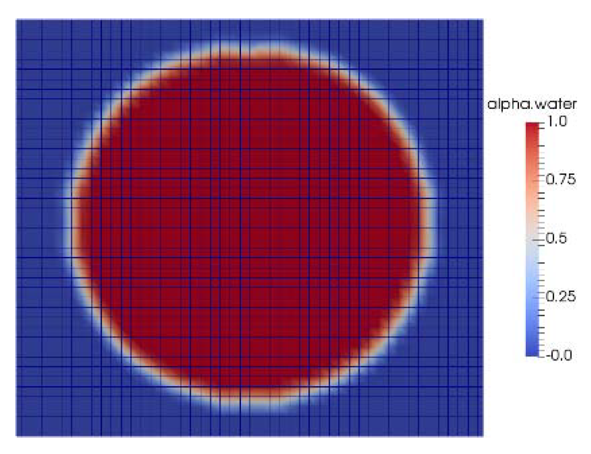
A simulation of a water droplet is taken as an example to validate the software, as shown in Figure 1. In the graph, the red color represents the fluid phase of the water, while the blue color denotes the fluid phase of air. The colors become blurred around the interphase, due to the magnitudes of the volume fraction, which ranges between 0 and 1.
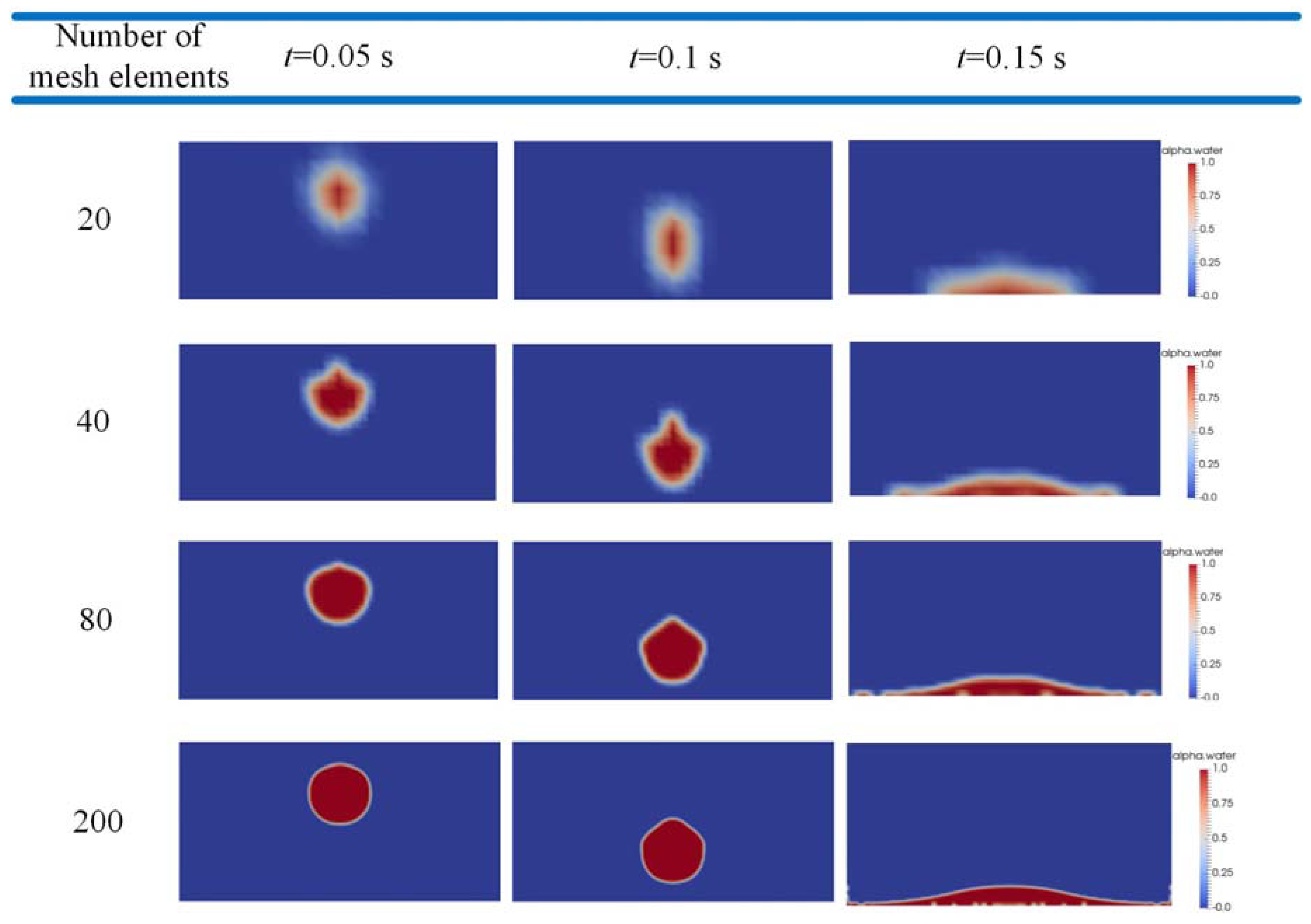
The mesh size was uniformly distributed in each direction within the boundaries of . Figure 2 displays simulations of water droplets with different numbers of mesh elements. The water droplet process was hard to capture when the coarse mesh cells were adopted. With reduced mesh cell size, the shape of the water droplets was more accurate. The results demonstrate that the developed software can successfully mimic the two fluid phases. Tests were conducted on an Intel Core i7-8700 K processor, with the simulation time presented in Table 1.
3. Observations of the Hydraulic Heave Phenomenon
The numerical simulations started with sample preparations, using the spherical particles in LIGGGHTS software. Figure 2 shows that tests in which the number of mesh elements was larger than 80, captured the air bubbles inside the water droplets during the simulation process. According to Table 1, the simulation time with 200 mesh elements was approximately 44 times the result with 80 mesh elements, without considering the solid phase. Hence, in this section, the size of the mesh cells in the CFD boundary equaled that adopted in Section 2 with 80 mesh elements. This size was used to model the multiphase fluids accurately and to reduce the computation effort.
3.1. Impact of Stratified Soils
Stratified soils are widely observed in natural lacustrine and marine deposits, and in engineering structures such as dam embankments. Gupta et al. [36] found that the permeability of soils constructed from clay in the top layer and sand in the ground would decrease with the increase of the top layer thickness. However, when sand is present in the upper layer and clay is present in the bottom layer, the permeability of the soil skeleton increases with the increasing thickness in the top. This would have a decisive effect on the rate of fluid flow through porous media and an impact on the seepage failure mechanism. Hence, the simulations adopted two different groups of gap-graded particles to study the impact of permeability in the vertical direction on the development of the hydraulic heave phenomenon. One group had radii of 0.25 and 1 mm for the fine particles and coarse particles, respectively, while the other one had radii of 0.5 and 1 mm for the fine particles and coarse particles, respectively.
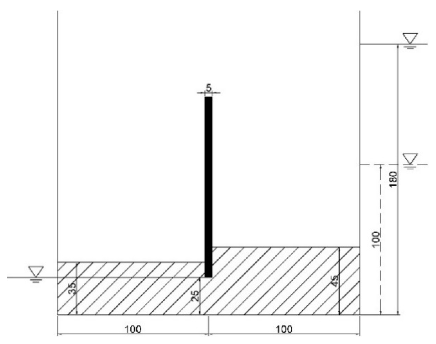
This section presents the tests that were performed in the saturated condition with three different specimens. Sample A refers to a uniform condition constructed with only one binary-sized particle, with radii of 0.25 and 1 mm. The other specimens were prepared with two layers of gap-graded particles, denoted as samples B and C, respectively. The condition of sample B was , whereas the condition of sample C was , where and denote the permeability coefficient of the top and bottom layers, respectively. This work determined the interface of the layers as the bottom of the retaining wall. Figure 3 depicts the initial configuration of the specimen, which measured 0.02 m in the y direction. Regarding a larger excavation, the seepage failure of the soil in front of sheet pile walls could be treated as a two-dimensional problem. Table 2 presents the information of samples.
After the samples were prepared, the system was submerged in fluid to observe the heave phenomenon. El Shamy and Zeghal [37] examined the impact of shear moduli on the steady-state response of pore fluid and particles subjected to upward fluid flow. For the moduli of and Pa, they found that the results of the tests were consistent and only observed minor local variations. Hence, Young’s modulus was selected as 5 MPa to reduce the computational effort. Table 3 gives the coefficients of parameters used in the simulations.
Tests were conducted by setting different hydraulic conditions at the two sides of the retaining wall. The simulations defined the left side as the downstream side, with the water table set to 0.025 m. Regarding the upstream side, this was selected as two different hydraulic heads (h) to study the impact of the hydraulic gradient, as shown in Figure 3.
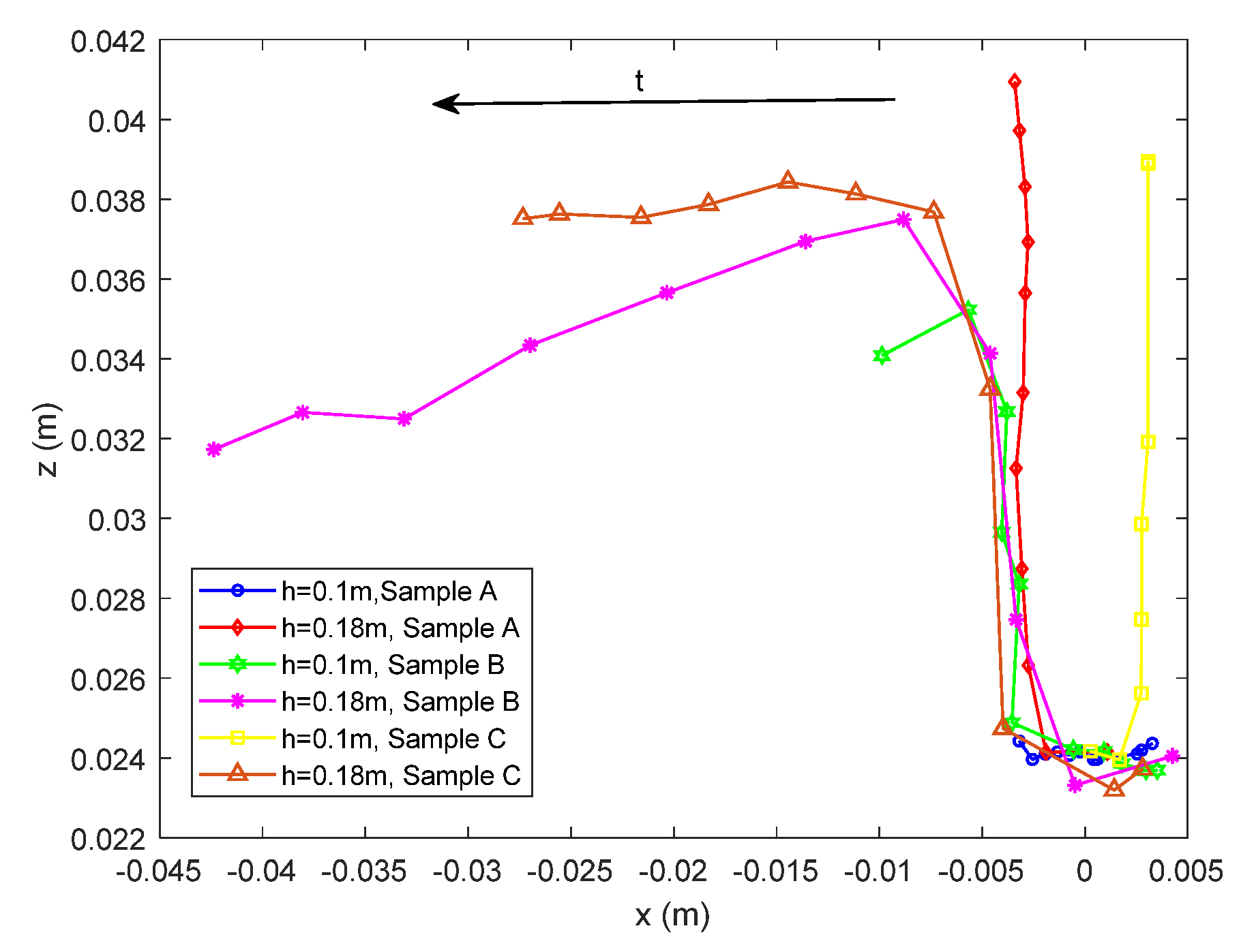
The critical characteristic of heave failure is the migration of particles inside the soil skeleton. Hence, Figure 4 portrays the particle trajectory to observe the seepage impact. Particles in the graph represent those located on the upstream side, which experience the largest displacement during the erosion process. The results indicate that a higher hydraulic gradient would result in severe seepage failure. Compared with the results of other samples, sample A produced the least transportation of particles, demonstrating that the erosion resistance increased with the increase of fine particles. Regarding the stratified specimens, sample B induced a higher detachment of particles than sample C.
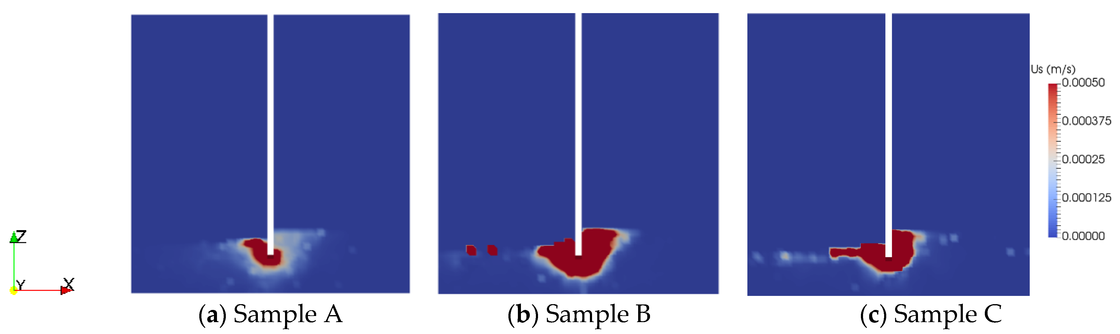
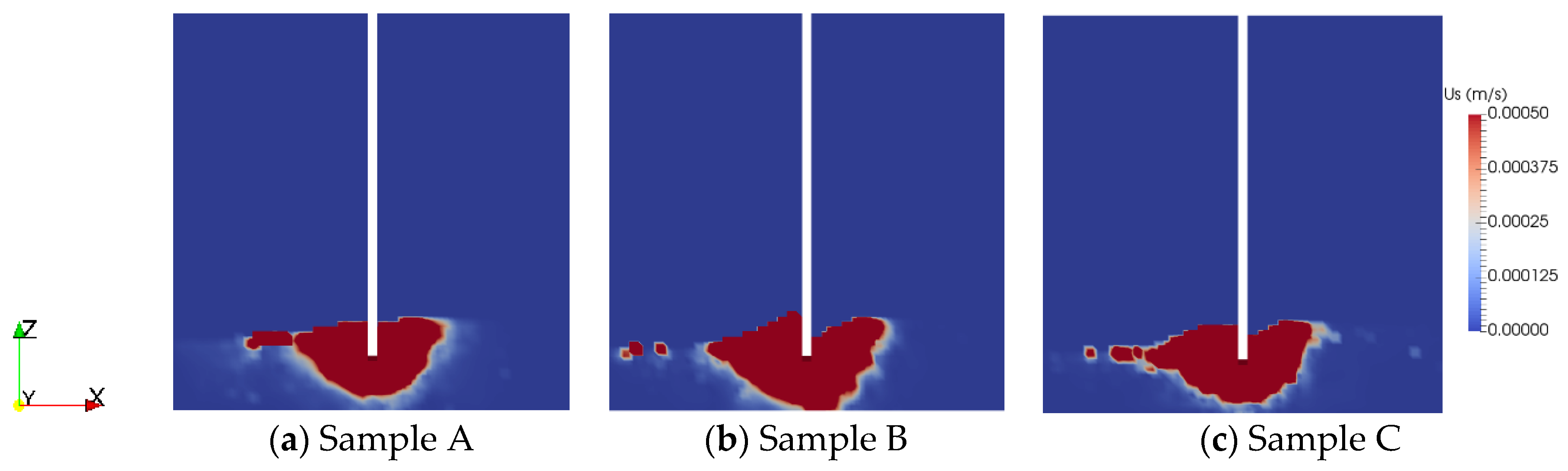
Figure 5 and Figure 6 display the distribution of the particle velocity at t = 1.0 s under different h values. The system showed faster particle speed for the region adjacent to the retaining wall. Moreover, the graphs show that sample A induces a relatively lower particle velocity value. Similar to the observations of Tanaka [38], sample B produced a significant hydraulic heave phenomenon, depending on the higher magnitude of the particle velocity. The results indicate that the top layer, which has a larger permeability coefficient, would result in a severe heave phenomenon.
3.2. Impact of Unsaturated Condition
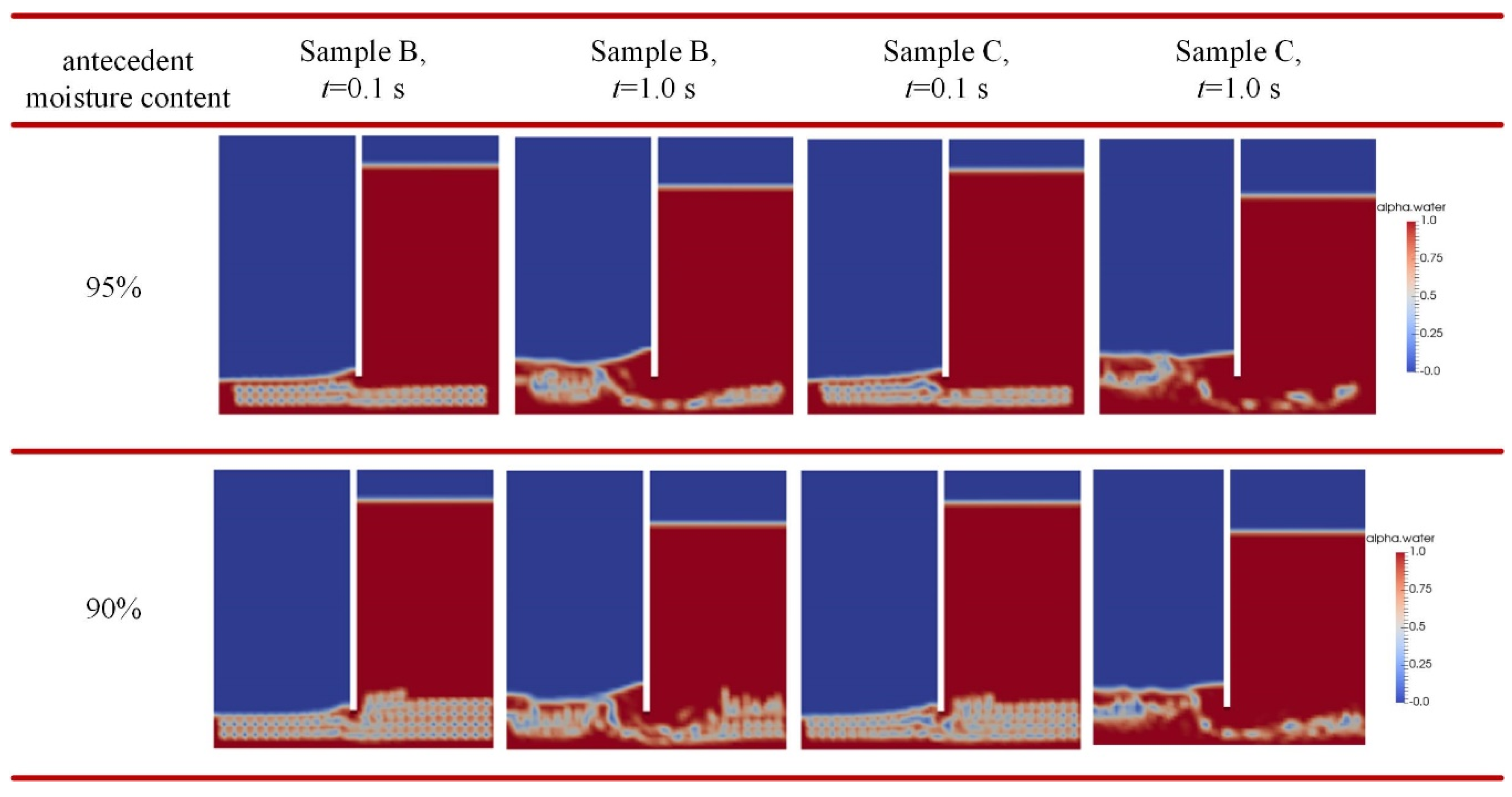
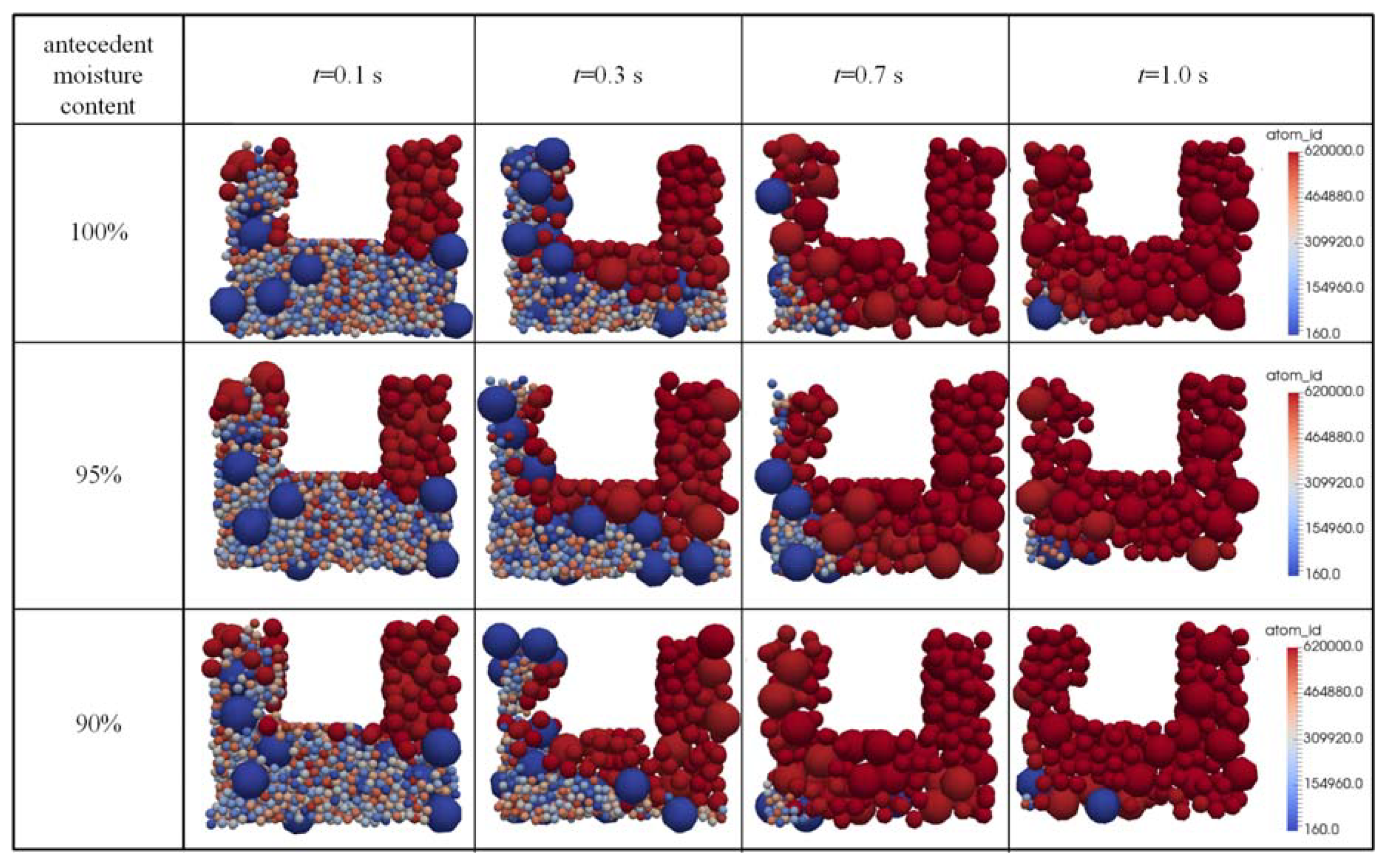
The above investigations demonstrate that the stratified soil skeleton would influence the occurrence of the heave phenomenon. This section further studies the erosion mechanism by considering air bubbles inside the system. The air bubbles, with the size of 0.005 m, were uniformly generated inside the specimen within the height of 0.0325 m in order to change the water content. The antecedent moisture content was estimated as the total volume of water inside the skeleton divided by the volume of the system. Tests were conducted under h = 0.18 m with moisture contents of 90% and 95%, respectively. Figure 7 gives the multiphase fluid flow behavior for different moisture contents. The results indicate that the fluid flow alters the shape of air bubbles and discharges the air bubbles from the downstream side. Regarding sample C, due to the coarse soil skeleton, the discharge rate of the air bubbles was larger in comparison with the results of sample B, as seen by the behavior at 1.0 s.
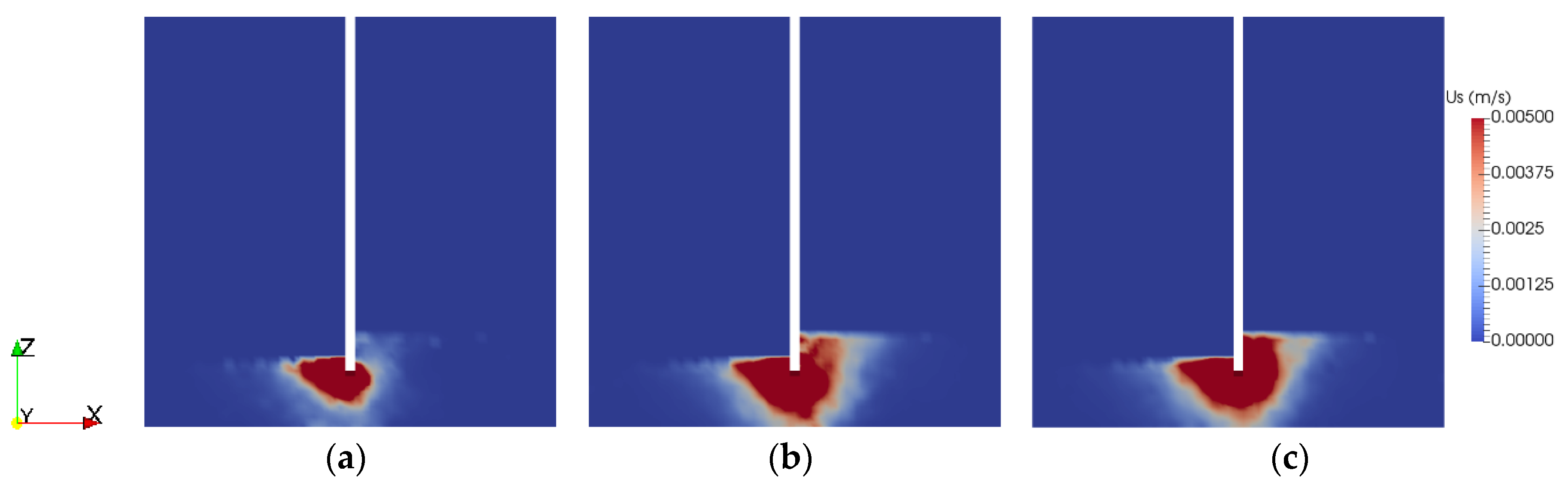
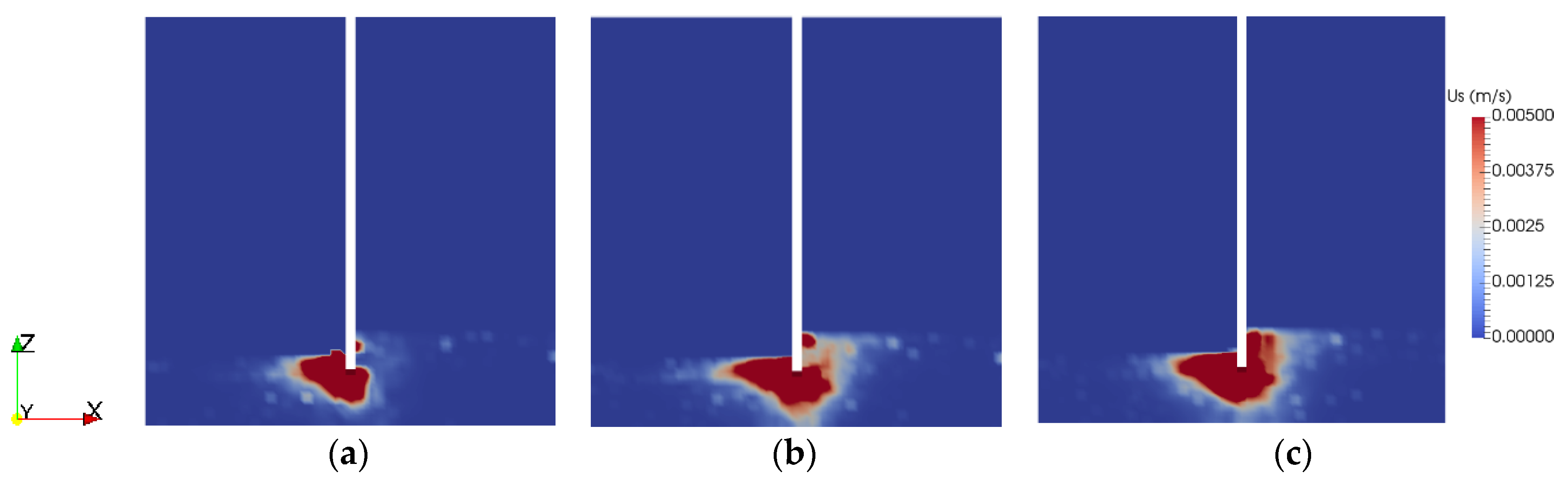
Taking t = 0.1 s as an example, Figure 8 and Figure 9 show the particle velocity fields of the two specimens to investigate the impact of air bubbles on the transportation of particles. For each simulation, the peak magnitude of the particle velocity occurred around the retaining wall. Moreover, the particle velocity was increased with an increase in the content of air bubbles. The results were similar to the work of Sakai and Maeda [31], which indicated that soil with lower antecedent moisture content would induce a severe seepage phenomenon at early stages.
Figure 10 depicts the spatial distribution of particle displacement to show the heave phenomenon at t = 1.0 s. The results are consistent with the particle velocity behavior. The graphs show that sample B containing more bubbles produces a great number of particles with higher displacement. According to Figure 10b, the influence of moisture content on the hydraulic heave phenomenon was negligible for sample C. The results indicate that the air bubbles in the fine soil skeleton would have a more significant impact on the seepage failure than those in a coarse soil skeleton.
4. Discussions on the Development of Heave Failure
Section 3 shows that the fluid flow has a significant impact on the particle velocity and the displacement field. This section aims to interpret the impact of antecedent moisture content on the occurrence of heave failure from particle-scale observations of internal structure and force. Based on the spatial distribution of the particle velocity and particle displacement, sample B produced a relatively significant seepage phenomenon under the impact of multiphase fluid flows, which was selected to investigate the erosion mechanism with air bubbles.
4.1. Spatial Distribution of Internal Structure
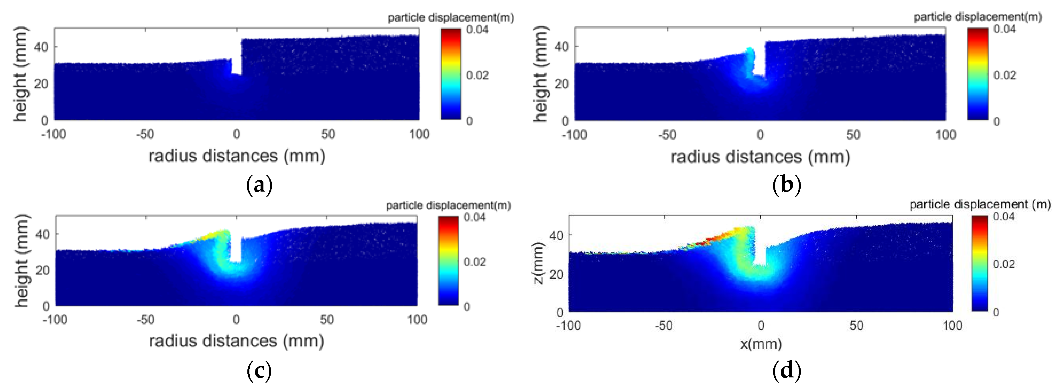
Figure 11 portrays the temporal and spatial distribution of the particle displacement for the specimen with 90% moisture content in order to study the development of the hydraulic heave phenomenon. At t = 0.1 s, the seepage impact formed flow paths around the boundary, inducing the occurrence of the boiling phenomenon. An obvious heave phenomenon was observed from t = 0.3 s onwards.
The above results indicate that the fluid flow would influence the transportation of particles. A central plane inside the specimen with dimensions of was selected and taken as an example to show the detailed redistribution of particles under seepage impact, as shown in Figure 12. The graphs display the obvious detachment of particles and suggest that the erosion phenomenon starts with particles adjacent to the wall on the downstream side and then regresses to the upstream side, resulting in the formation of flow channels. The results are consistent with the particle velocity behavior. The fluid flow results in a more serious loss of particles with increasing content of air bubbles inside the soil skeleton.
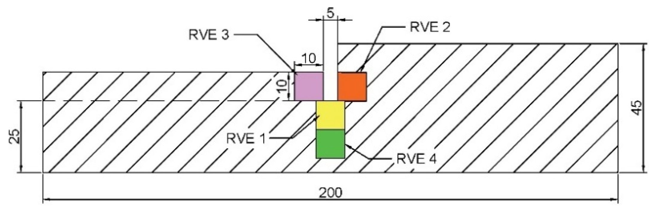
The spatial distribution of the soil skeleton demonstrates that the seepage impact induces the redistribution of particles and results in different particle interactions. According to the definition of the internal structure (fabric) proposed by Brewer [39], the results imply that the fluid flow alters the internal structure of the system due to the change of porosity and rearrangement of particles during the erosion process, and influences the erosion resistance and shear resistance of the system. Since the redistribution of particles mainly appears around the boundary, four different representative volume elements (RVE), with the dimensions of , were selected to study the characteristics of the internal structure during erosion. These elements were located underneath the boundary, and on the left and right sides of the retaining wall, as shown in Figure 13.
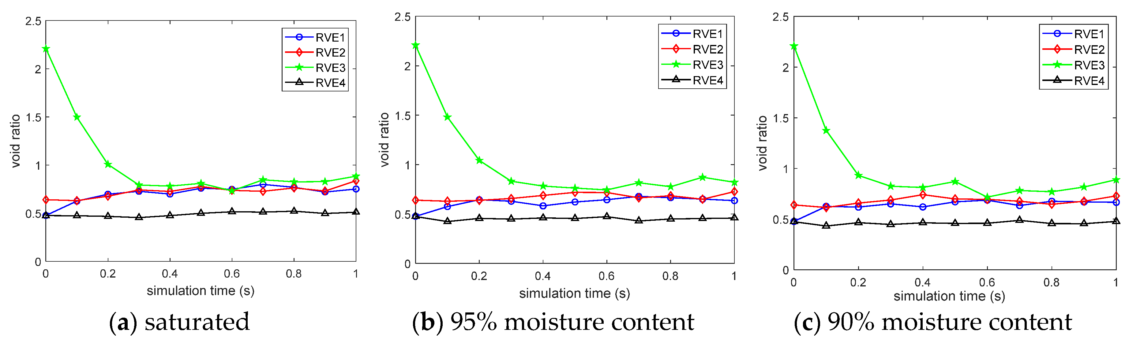
Figure 14 presents the evolution of the void ratio for the different elements. Similar behavior was observed for the specimen with different antecedent moisture contents. Regarding the element near the free surface on the downstream side, the void ratio was higher at the initial stage due to the coarse soil skeleton. During erosion, the fluid flow triggered the movement of fine particles to fill this element and induced a reduction of the void ratio due to the occurrence of heave or boiling failure. The detachment of particles would affect the loss of particles on the upstream side and form flow channels, which can increase the porosity on the upper parts of flow paths.
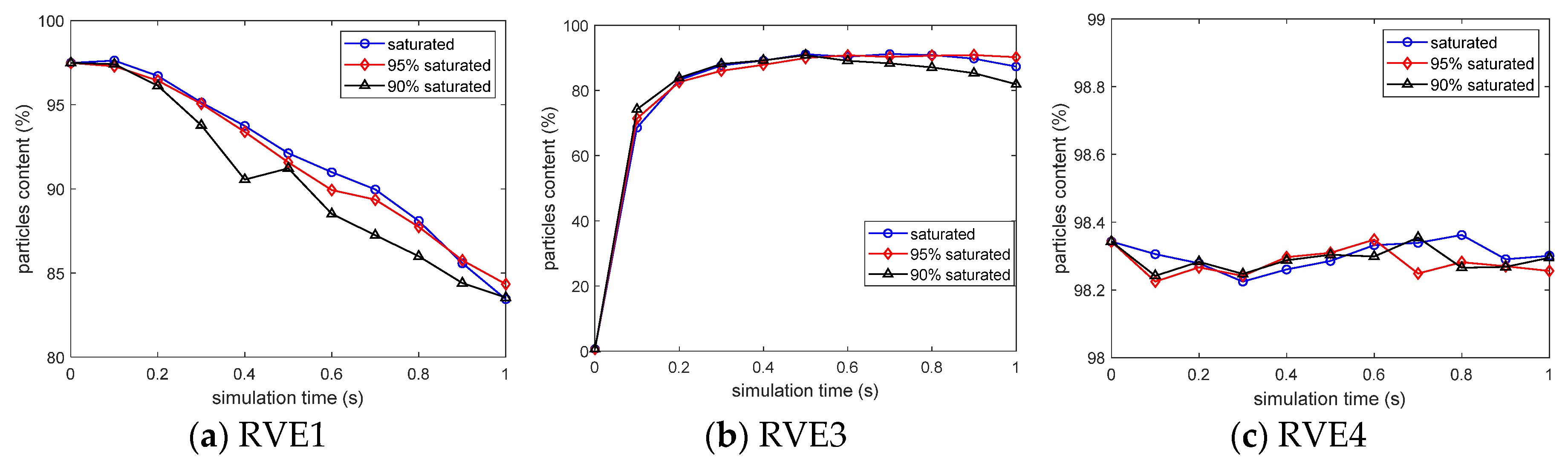
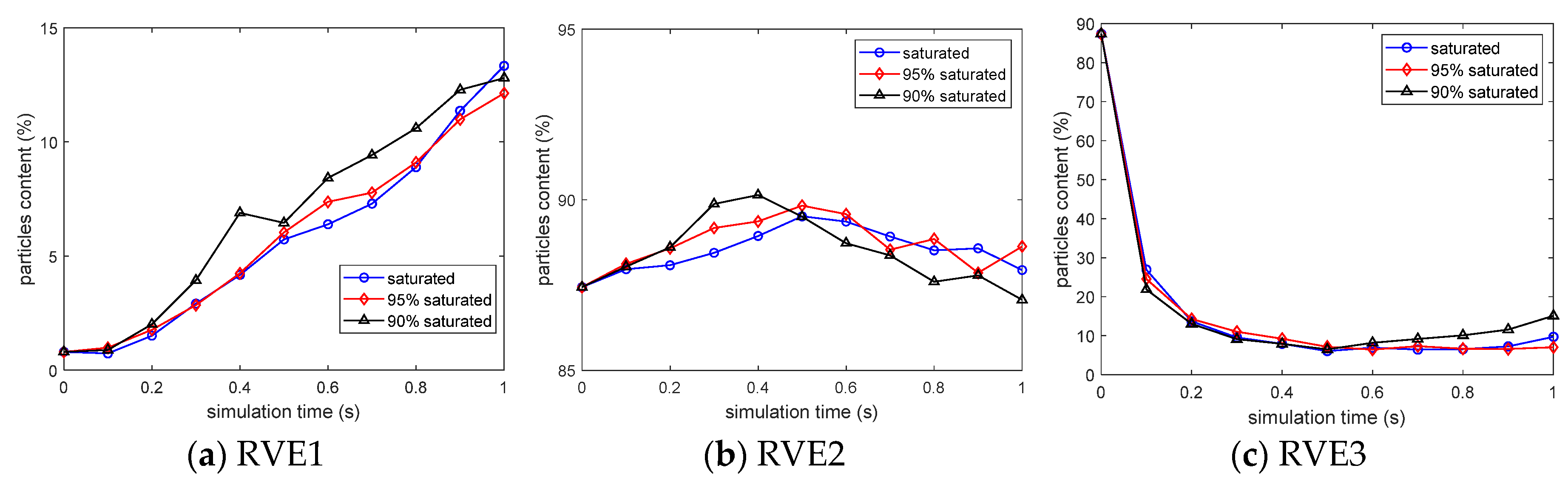
To further analyze the erosion mechanism, the temporal changes of particle size distribution inside the elements were tracked and recorded, with the results displayed in Figure 15 and Figure 16. The particles of 0.00025 and 0.0005 m were not contained in elements RVE2 and RVE4, respectively. The impact of air bubbles was slight for the element near the base of the system. The loss of fine particles was more significant around the wall. The graphs imply that the seepage phenomenon starts at the free surface on the downstream side (RVE3) and induces a drop in the content of the 0.0005 m particles due to fluid flow, which results in a rapid increase in the content of fine particles. Compared with the results of other samples, the specimen with 90% antecedent moisture content produced a serious reduction of fine particles in the region below the retaining wall, which caused further movement of particles on the upstream side and increased the content of coarse particles in RVE2, particularly at the initial stages. The results indicate that the impact of multiphase fluid flows would induce rapid occurrence of the heave phenomenon and influence the stability of the system at an early stage.
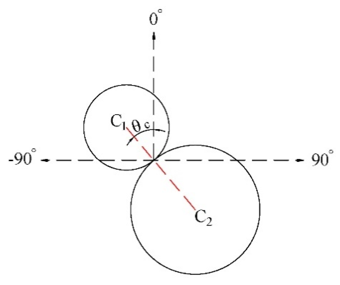
The redistribution of particles would also impact the rearrangement of particle interactions. The probability distribution of the contact orientation was examined with different saturated conditions. Figure 17 defines the contact orientation in this study. The RVE1 element showed significant differences in the contents of the particles. This element was selected to study the behavior of contact orientation during erosion, with the results displayed in Figure 18. Compared with the initial results, the seepage impact increased the probability of contact orientation within the span of . The results indicate that the fluid flow in the soil skeleton with lower moisture content induces the rotation of inter-particle contacts in a relatively vertical direction, particularly in the initial stage, which may exacerbate the occurrence of the boiling phenomenon.
4.2. Spatial Distribution of Drag Force
Section 4.1 shows that the unsaturated condition would influence the internal structure of the system. This section further studied the impact of air bubbles on the seepage failure mechanism based on the force field observations. The simulations investigated the drag force as the interaction force between fluid and particles using the Di Felice model with the following equations [40]:
where is the drag coefficient and is the Reynolds number; is the diameter of the considered particle; and and are the drag force and volume of each particle, respectively.
The transportation of particles occurred when the seepage force exceeded the weight of the soil bulk. Hence, the ratio between the drag force and corresponding soil weight, shown as , was investigated to analyze the occurrence of seepage failure. According to Figure 15 and Figure 16, the impact of air bubbles on the movement of particles was more significant in the initial stages. Thus, the temporal–spatial distribution of drag force was studied within the simulation time of 0.4 s. Figure 19, Figure 20 and Figure 21 portray the results of in the central region of the system for sample B. For each simulation, the peak magnitude of was observed underneath the retaining wall at the initial stage. Moreover, the values of were increased around the boundary, with a reduction of the antecedent moisture content of the system, which caused higher particle velocities and aggravated the movement of particles, resulting in a significant seepage failure phenomenon.
5. Conclusions
This paper studied the occurrence of heave failure under multiphase fluid flow using the CFD-DEM approach. The interFoam solver of OpenFOAM software was developed in the CFD-DEM engine to capture the fluid properties in the two fluid phases. Similar to the experimental results reported in the literature, the specimen with the larger permeability coefficient in the upper layer produced significant heave failure. This study prepared samples with different moisture contents in order to examine the impact of air bubbles on the development of the hydraulic heave phenomenon. The system with increasing content of air bubbles presented a larger particle velocity concentrated around the boundary, which would cause a significant heave phenomenon at the initial stage. Moreover, regarding the stratified soils, the impact of air bubbles in a coarse skeleton on the heave phenomenon is smaller than that contained in fine soil. Special attention was paid to the spatial distribution of the internal structure and drag force to investigate the erosion mechanism. According to the spatial distribution of particles, it is suggested that the fluid flow involving the air phase produces a serious loss of fine particles around the retaining wall and causes rearrangement of the interactions. Based on the contact orientation behavior, the impact of air bubbles produced a higher probability in the vertical direction for the region below the retaining wall, particularly at t = 0.1 s. With the development of seepage erosion, the influence of air bubbles on the migration of particles and the contact orientation was not that significant. The spatial distribution of drag force was further investigated to analyze the occurrence of seepage failure at the initial stages of the seepage process. Compared with the saturated condition, samples with a great number of air bubbles caused a higher ratio of drag force and soil weight adjacent to the wall, increasing the velocity of particles and rapidly inducing severe seepage failure. The results suggest that the existence of air bubbles may exacerbate the process of heave or boiling failure and affect the infrastructure stability at an early stage.
Funding
This research received no external funding.
Conflicts of Interest
The author declares no conflict of interest.
References
- McNamee, J. Seepage into a Sheeted Excavation. Géotechnique 1949, 1, 229–241. [Google Scholar] [CrossRef]
- Foster, M.; Fell, R.; Spannagle, M. The statistics of embankment dam failures and accidents. Can. Geotech. J. 2000, 37, 1000–1024. [Google Scholar] [CrossRef]
- Terzaghi, K. Theoretical Soil Mechanics; Wiley: Hoboken, NJ, USA, 1943. [Google Scholar]
- Fleshman, M.S.; Rice, J.D. Laboratory modeling of the mechanisms of piping erosion initiation. J. Geotech. Geoenviron. Eng. 2014, 140, 04014017. [Google Scholar] [CrossRef]
- Xie, Q.; Liu, J.; Han, B.; Li, H.; Li, Y.; Li, X. Critical hydraulic gradient of internal erosion at the soil-structure interface. Processes 2018, 6, 92. [Google Scholar] [CrossRef] [Green Version]
- Chang, D.; Zhang, L. Critical hydraulic gradients of internal erosion under complex stress states. J. Geotech. Geoenviron. Eng. 2013, 139, 1454–1467. [Google Scholar] [CrossRef]
- Miura, K.; Supachawarote, C.; Ikeda, K. Estimation of 3D seepage force inside cofferdam regarding boiling type of failure. In Proceedings of the Geotech-Year 2000 Developments in Geotechnical Engineering, Bangkok, Thailand, 27–30 November 2000; pp. 371–380. [Google Scholar]
- Tanaka, T. Boiling occurred within a braced cofferdam due to two dimensionally concentrated seepage flow. In Proceedings of the 3rd International Symposium, Geotechnical Aspects of Underground Construction in Soft Ground, Toulouse, France, 23–25 October 2002; pp. 33–38. [Google Scholar]
- Tanaka, T.; Tomoya, K.; Shigeru, N.; Daisuke, H. Characteristics of seepage failure of soil under various flow conditions. In Proceedings of the Nineteenth International Offshore and Polar Engineering Conference, Osaka, Japan, 21–26 June 2009; pp. 21–26. [Google Scholar]
- Tanaka, T.; Verruijt, A. Seepage failure of sand behind sheet piles—The mechanism and practical approach to analyze. Soils Found. 1999, 39, 27–35. [Google Scholar] [CrossRef] [Green Version]
- Moffat, R.; Fannin, R.J.; Garner, S.J. Spatial and temporal progression of internal erosion in cohesionless soil. Can. Geotech. J. 2011, 48, 399–412. [Google Scholar] [CrossRef]
- Luo, Y.; Nie, M.; Xiao, M. Flume-scale experiments on suffusion at bottom of cutoff wall in sandy gravel alluvium. Can. Geotech. J. 2017, 54, 1716–1727. [Google Scholar] [CrossRef] [Green Version]
- Wan, C.F.; Fell, R. Investigation of rate of erosion of soils in embankment dams. J. Geotech. Geoenviron. Eng. 2004, 130, 373–380. [Google Scholar] [CrossRef]
- Kawano, K.; O’Sullivan, C.; Shire, T. Using DEM to assess the influence of stress and fabric inhomogeneity and anisotropy on susceptibility to suffusion. In Proceedings of the 8th International Conference on Scour and Erosion, Oxford, UK, 12–15 September 2016; pp. 85–94. [Google Scholar]
- Shire, T.; O’Sullivan, C.; Hanley, K.J.; Fannin, R.J. Fabric and effective stress distribution in internally unstable soils. J. Geotech. Geoenviron. Eng. 2014, 140, 04014072. [Google Scholar] [CrossRef] [Green Version]
- Maeda, K.; Sakai, H. Seepage failure and erosion of ground with air bubble dynamics. Soil Behav. Geo-Micromech. 2010. [Google Scholar] [CrossRef]
- Swain, S.; Mohanty, S. A 3-dimensional Eulerian—Eulerian CFD simulation of a hydrocyclone. Appl. Math. Model. 2013, 37, 2921–2932. [Google Scholar] [CrossRef]
- Chen, S.; Doolen, G.D. Lattice Boltzmann method for fluid flows. Annu. Rev. Fluid Mech. 1998, 30, 329–364. [Google Scholar] [CrossRef] [Green Version]
- Griffiths, D.V.; Fenton, G.A. Seepage beneath water retaining structures founded on spatially random soil. Géotechnique 1993, 43, 577–587. [Google Scholar] [CrossRef] [Green Version]
- Koltuk, S.; Song, J.; Iyisan, R.; Azzam, R. Seepage failure by heave in sheeted excavation pits constructed in stratified cohesionless soils. Front. Struct. Civ. Eng. 2019, 13, 1415–1431. [Google Scholar] [CrossRef]
- Benmebarek, N.; Benmebarek, S.; Kastner, R. Numerical studies of seepage failure of sand within a cofferdam. Comput. Geotech. 2005, 32, 264–273. [Google Scholar] [CrossRef]
- Zou, Y.-H.; Chen, Q.; Chen, X.-Q.; Cui, P. Discrete numerical modeling of particle transport in granular filters. Comput. Geotech. 2013, 47, 48–56. [Google Scholar] [CrossRef]
- Huang, Q.-F.; Zhan, M.-L.; Sheng, J.-C.; Luo, Y.-L.; Su, B.-Y. Investigation of fluid flow-induced particle migration in granular filters using a DEM-CFD method. J. Hydrodyn. 2014, 26, 406–415. [Google Scholar] [CrossRef]
- Kawano, K.; Shire, T.; O’Sullivan, C. Coupled DEM-CFD analysis of the initiation of internal instability in a gap-graded granular embankment filter. EPJ Web Conf. 2017, 140, 10005. [Google Scholar] [CrossRef] [Green Version]
- Guo, Y.; Yang, Y.; Yu, X.B. Influence of particle shape on the erodibility of non-cohesive soil: Insights from coupled CFD–DEM simulations. Particuology 2018, 39, 12–24. [Google Scholar] [CrossRef]
- Zou, Y.; Chen, C.; Zhang, L. Simulating progression of internal erosion in gap-graded sandy gravels using coupled CFD-DEM. Int. J. Géoméch. 2020, 20, 04019135. [Google Scholar] [CrossRef]
- Tao, H.; Tao, J. Quantitative analysis of piping erosion micro-mechanisms with coupled CFD and DEM method. Acta Geotech. 2017, 12, 573–592. [Google Scholar] [CrossRef]
- Bannari, R.; Kerdouss, F.; Selma, B.; Bannari, A.; Proulx, P. Three-dimensional mathematical modeling of dispersed two-phase flow using class method of population balance in bubble columns. Comput. Chem. Eng. 2008, 32, 3224–3237. [Google Scholar] [CrossRef]
- Rusche, H. Computational Fluid Dynamics of Dispersed Two-Phase Flows at High Phase Fractions. Ph.D. Thesis, University of London, London, UK, 2002. [Google Scholar]
- Kodaka, T.; Asaoka, A. Formation of air bubbles in sandy soil during seepage process. J. JSCE 1994, 487, 129–138. (In Japanese) [Google Scholar]
- Sakai, H.; Maeda, K. Seepage Failure and Erosion Mechanism of Granular Material with Evolution of Air Bubbles Using SPH. In Proceedings of the 6th International Conference on Micromechanics of Granular Media, Golden, CO, USA, 13–17 July 2009. [Google Scholar]
- LIGGGHTS. LIGGGHTS (R)-Public Documentation, Version 3.X. Available online: http://www.cfdem.com (accessed on 18 February 2015).
- OpenFOAM. OpenFOAM—The Open Source CFD Toolbox. The OpenFOAM Foundation, 2015. Available online: http://www.openfoam.org (accessed on 22 May 2015).
- Cundall, P.A.; Strack, O.D.L. A discrete numerical model for granular assemblies. Géotechnique 1979, 29, 47–65. [Google Scholar] [CrossRef]
- Xiao, Q.; Wang, J.-P. CFD–DEM simulations of seepage-induced erosion. Water 2020, 12, 678. [Google Scholar] [CrossRef] [Green Version]
- Gupta, P.; Alam, J.; Muzzammil, M. Influence of thickness and position of the individual layer on the permeability of the stratified soil. Perspect. Sci. 2016, 8, 757–759. [Google Scholar] [CrossRef] [Green Version]
- El Shamy, U.; Zeghal, M. Coupled continuum-discrete model for saturated granular soils. J. Eng. Mech. 2005, 131, 413–426. [Google Scholar] [CrossRef]
- Tanaka, T.; Kageyama, T.; Nagai, S. Seepage failure test of sand within cofferdam-test apparatus and seepage flow pattern. In Proceedings of the 40th Geotechnical Engineering Symposium on New Problems and New Technology, New Delhi, India, 7–11 April 1995; pp. 323–330. [Google Scholar]
- Brewer, R. Fabric and mineral analysis of soils. Soil Sci. 1965, 100, 73. [Google Scholar] [CrossRef]
- Di Felice, R. The voidage function for fluid-particle interaction systems. Int. J. Multiph. Flow 1994, 20, 153–159. [Google Scholar] [CrossRef]
Figure 1.
An example of the gas–fluid phase definition.

Figure 2.
Simulation of water droplets with different numbers of mesh elements in the x direction.

Figure 3.
The initial configuration of the specimen (unit: mm).

Figure 4.
The behavior of the particle trajectory under different h values.

Figure 5.
Particle velocity behavior at t = 1.0 s with h = 0.1 m.

Figure 6.
Particle velocity behavior at t = 1.0 s with h = 0.18 m.

Figure 7.
The fluid flow behavior with h = 0.18 m.

Figure 8.
The particle velocity behavior for sample B at t = 0.1 s with antecedent moisture contents of (a) 100%, (b) 95%, and (c) 90%.
Figure 8.
The particle velocity behavior for sample B at t = 0.1 s with antecedent moisture contents of (a) 100%, (b) 95%, and (c) 90%.

Figure 9.
The particle velocity behavior for sample C at t = 0.1 s with antecedent moisture contents of (a) 100%, (b) 95%, and (c) 90%.
Figure 9.
The particle velocity behavior for sample C at t = 0.1 s with antecedent moisture contents of (a) 100%, (b) 95%, and (c) 90%.

Figure 10.
The spatial distribution of particle displacement at t = 1.0 s under h = 0.18 m.

Figure 11.
The spatial distribution of particle displacement for the sample with 90% moisture content at t = (a) 0.1, (b) 0.3, (c) 0.7, and (d) 1.0 s.
Figure 11.
The spatial distribution of particle displacement for the sample with 90% moisture content at t = (a) 0.1, (b) 0.3, (c) 0.7, and (d) 1.0 s.

Figure 12.
Spatial distribution of particles within the region measuring during erosion.

Figure 13.
The representative volume elements inside the system (unit: mm).

Figure 14.
The evolution of the void ratio during erosion for sample B.

Figure 15.
The evolution of the particle content for sample B at r = 0.00025 m.

Figure 16.
The evolution of the particle content for sample B at r = 0.0005 m.

Figure 17.
The contact orientation.

Figure 18.
The probability of contact orientation for the RVE1 element at t = (a) 0.1 and (b) 0.4 s.
Figure 18.
The probability of contact orientation for the RVE1 element at t = (a) 0.1 and (b) 0.4 s.

Figure 19.
The spatial distribution of soil weight () for the saturated sample at t = (a) 0.1, (b) 0.2, (c) 0.3, and (d) 0.4 s.
Figure 19.
The spatial distribution of soil weight () for the saturated sample at t = (a) 0.1, (b) 0.2, (c) 0.3, and (d) 0.4 s.

Figure 20.
The spatial distribution of for the sample with 95% moisture content at t = (a) 0.1, (b) 0.2, (c) 0.3, and (d) 0.4 s.
Figure 20.
The spatial distribution of for the sample with 95% moisture content at t = (a) 0.1, (b) 0.2, (c) 0.3, and (d) 0.4 s.

Figure 21.
The spatial distribution of for the sample with 90% moisture content at t = (a) 0.1, (b) 0.2, (c) 0.3, and (d) 0.4 s.
Figure 21.
The spatial distribution of for the sample with 90% moisture content at t = (a) 0.1, (b) 0.2, (c) 0.3, and (d) 0.4 s.


Table 1.
Simulation times for different numbers of mesh elements.
| Number of Mesh Elements | 20 | 40 | 80 | 200 |
| Simulation Time (s) | 29 | 60 | 490 | 21,524 |
Table 2.
The prepared samples.
| Sample Information | Sample A | Sample B | Sample C |
|---|---|---|---|
| Number of Particles | 816,692 | 550,806 | 237,597 |
Table 3.
Properties of particles and boundaries.
| Parameters | Magnitudes |
|---|---|
| Young’s Modulus | 5 MPa |
| Friction Coefficient | 0.5 |
| Poisson’s Ratio | 0.45 |
| Restitution Coefficient | 0.1 |
| Kinematic Viscosity of Water | 1 × 10⁻⁶ m2/s |
| Density of Water | 1000 kg/m3 |
| Kinematic Viscosity of Air | 1.506 × 10⁻⁵ m2/s |
| Density of Air | 1.2041 kg/m3 |
© 2020 by the author. Licensee MDPI, Basel, Switzerland. This article is an open access article distributed under the terms and conditions of the Creative Commons Attribution (CC BY) license (http://creativecommons.org/licenses/by/4.0/).
Share and Cite
MDPI and ACS Style
Xiao, Q. Simulating the Hydraulic Heave Phenomenon with Multiphase Fluid Flows Using CFD-DEM. Water 2020, 12, 1077. https://doi.org/10.3390/w12041077
AMA Style
Xiao Q. Simulating the Hydraulic Heave Phenomenon with Multiphase Fluid Flows Using CFD-DEM. Water. 2020; 12(4):1077. https://doi.org/10.3390/w12041077
Chicago/Turabian StyleXiao, Qiong. 2020. "Simulating the Hydraulic Heave Phenomenon with Multiphase Fluid Flows Using CFD-DEM" Water 12, no. 4: 1077. https://doi.org/10.3390/w12041077
Note that from the first issue of 2016, this journal uses article numbers instead of page numbers. See further details here.