Characterizing the Water Storage Capacity and Hydrological Role of Mountain Peatlands in the Arid Andes of North-Central Chile

Abstract

High-altitude peatlands in the Andes, i.e., bofedales, play an essential role in alpine ecosystems, regulating the local water balance and supporting biodiversity. This is particularly true in semiarid Chile, where bofedales develop near the altitudinal and hydrological limits of plant life. The subterranean geometry and stratigraphy of one peatland was characterized in north-central Chile using Electrical Resistivity Tomography (ERT), Ground Penetrating Radar (GPR) and core extraction. Two sounding locations, two transversal and one longitudinal profile allowed a 3D interpretation of the bofedal’s internal structure. A conceptual model of the current bofedal system is proposed. Geophysical results combined with porosity measurements were used to estimate the bofedal water storage capacity. Using hydrological data at the watershed scale, implications regarding the hydrological role of bofedales in the semiarid Andes were then briefly assessed. At the catchment scale, bofedal water storage capacity, evapotranspiration losses and annual streamflow are on the same order of magnitude. High-altitude peatlands are therefore storing a significant amount of water and their impact on basin hydrology should be investigated further.

1. Introduction

Peat accumulating wetlands in the Andes, i.e., bofedales, are critical for livestock grazing in the highlands from Venezuela to Chile [1,2] and play a crucial role in sustaining a unique diversity of endemic and rare biota [3,4]. One-third of the threatened bird species and mammals in the Andes depend upon bofedales for water, nesting and grazing. Whilst bofedales are generally small-sized, they likely impact regional carbon stocks due to their large number and relatively deep peat layers [5,6,7]. Bofedales are increasingly being recognized as key regulators of the local water balance [8], and regional hydrology is likely influenced by their water storage capacity and retardation of surface flow [9]. The hydrological role of bofedales is likely very important for downstream urban and agricultural activities [10].

Andean bofedales develop near the hydrological and altitudinal limits for plant life [11]. Surrounding areas are characterised by high-velocity winds, intense solar radiation, a short growing season, daily frost and a seasonal snow cover, all of which are strong impediments to vegetation development [4,9,12]. They form in relatively flat areas along small watercourses or ponds, and are occasionally expanded by human intervention. Whilst most bofedales are characterised by saturated sediments throughout the year [13], in a few cases, they are ephemeral features. As they are dependent on water supply for their development [14], and are temperature-limited depending on the tolerance of the local vegetation, their elevation band varies along the Andes. In general, in the central Andes (16° S), they exist between 4000 and 5000 m a.s.l., whereas in the southern Andes (27° S) they generally occupy a lower elevation band (2000–3500 m a.s.l.) [14,15].

Bofedales found in the southern Andes (south of 24° S) exist in arid and semiarid conditions, which mean they fill a distinct environmental niche in the continuum of mountain peatland (peat accumulating wetland) environments. Due to the logistical complexity of accessing these areas, the internal structure, hydrological role and development processes of these Andean peatlands are poorly understood in comparison to Northern Hemisphere peatlands. Nearly all understanding of peatland processes is based on Northern Hemisphere peatlands (e.g., [16,17,18,19,20,21]), where climatic conditions are vastly different. Although bofedales have been referred to as “highland bogs” [22,23], they are different from the Northern Hemisphere bogs because they are generally not ombrogenous, nor covered by mosses, and are at the limits of complex plant survival. Ground Penetrating Radar (GPR) has been extensively used to characterize peatland structure [24], especially to identify the peatland base [25,26]. GPR was successfully used to quantify carbon stocks in high-altitude peatlands [6], while [24] used a combination of GPR and Electrical Resistivity Tomography (ERT) to enhance the hydrogeological understanding of a northern peatbog. Resistivity methods have been applied to peatlands in several studies [24,27,28,29,30,31,32,33]. One study mentioned above [6] focused on a peatland in the northern Andes, while all other studies are for peatlands outside of South America.

This study aims to understand the hydrological role of high Andean wetlands as water reservoirs. The internal structure and the water storage capacity of the bofedal are assessed using geophysical techniques. This study is the first to apply ERT and GPR to map the 3D underground structure of an arid region bofedal in the scientific literature. Likewise, this is the first assessment of the water storage capacity of an arid peatland to our knowledge. Using the results generated for the bofedal, we estimate the total water storage capacity offered by peatlands over the entire watershed to understand their hydrological role at the watershed scale.

2. Study Area

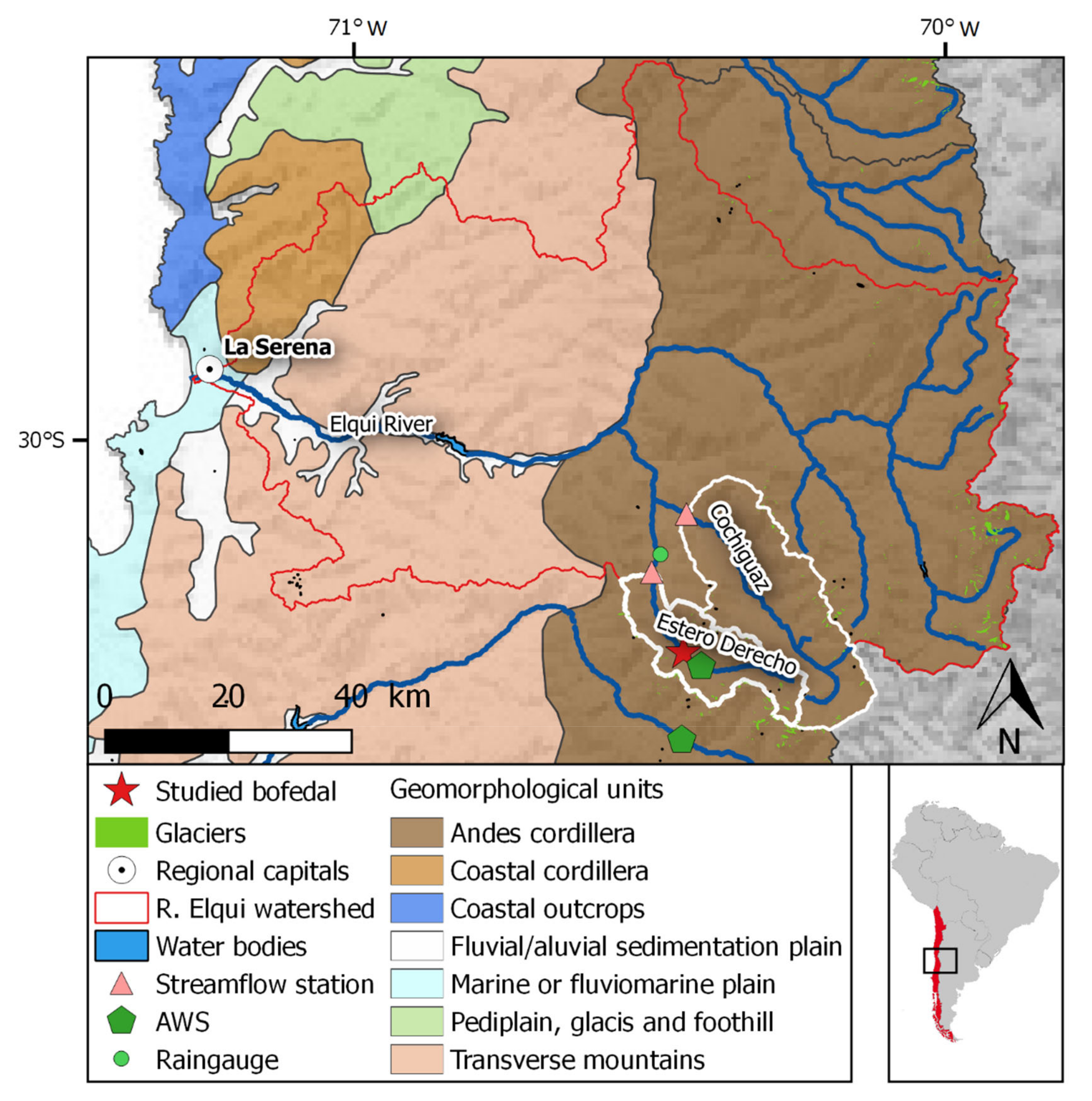
2.1. Geographical Context

The study area is located in north-central Chile (30° S), where the distance between the Pacific Ocean and the highest peaks of the Andes (>6000 m a.s.l.) is less than 150 km. This strong altitudinal gradient and intensive compression between the Nazca and South American tectonic plates, associated with a flat slab segment (between 28° S and 33° S, e.g., [34]), has resulted in the creation of major transverse valleys, such as the Elqui Valley in the Coquimbo Region (Figure 1). Together with two major valleys further north (Huasco and Copiapó), these watersheds drain the last northern perennial surface flow before the hyper arid systems of the Atacama Desert (northward 28° S).

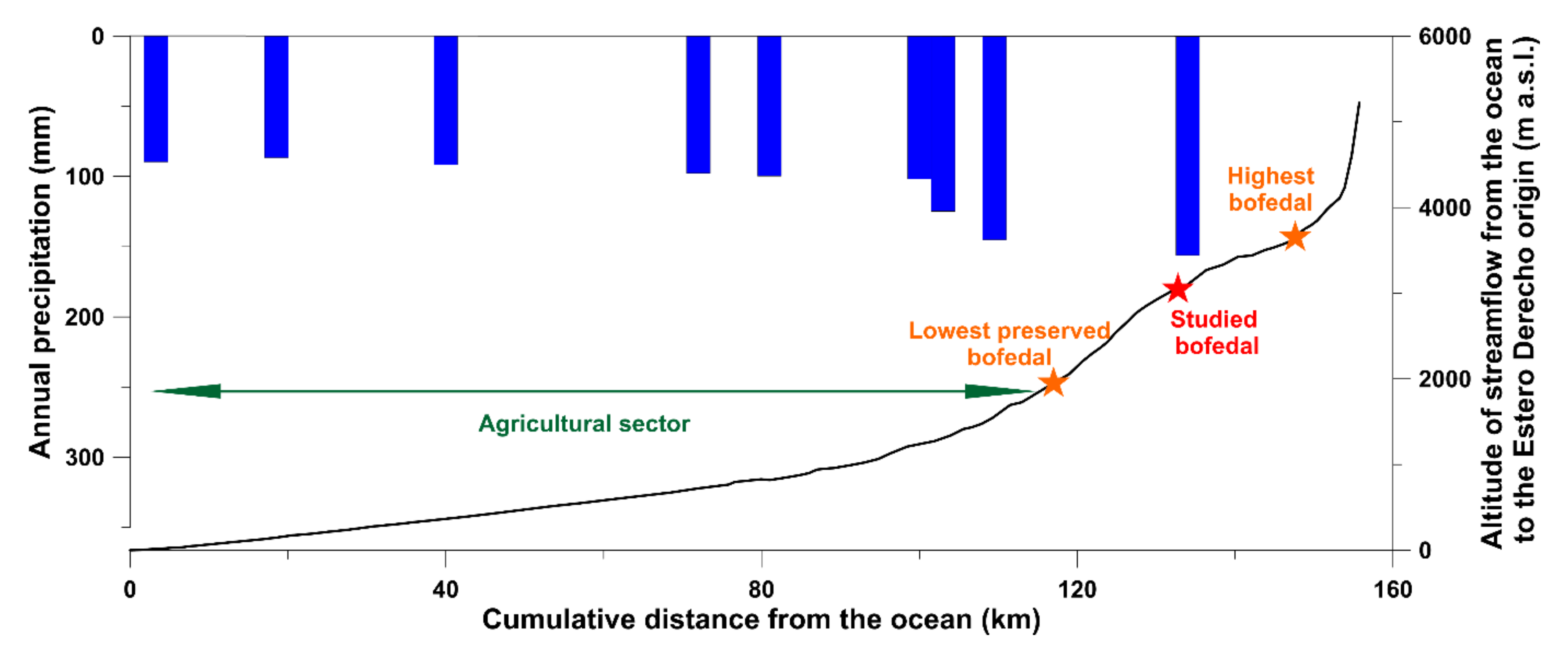
2.2. Climatic Context

Between 1870 and 1890, average precipitation was ~150 mm per year in La Serena (30° S, 142 m a.s.l.) [35,36]. Since 1870, a negative trend of −0.52 mm per year and reduction in rainfall by ~50% has been observed. In this region, precipitation generally increases with altitude (Figure 2), however there is a strong temporal variability linked to the El Niño Southern Oscillation (ENSO) at an inter-annual time scale [35] and the Pacific Decadal Oscillation [37] at a decadal time scale. More winter precipitation at higher altitudes enables the formation of a seasonal snowpack that completely melts in the following spring and summer seasons [35,38]. This snowpack governs annual streamflow volume in the main river channels [39]. Aside from snow melt and direct rainfall, perennial flows are maintained mainly by aquifers contained within the sediment filled valleys, as well as from debris-free and rock glaciers [35,40,41,42].

2.3. Geological Context

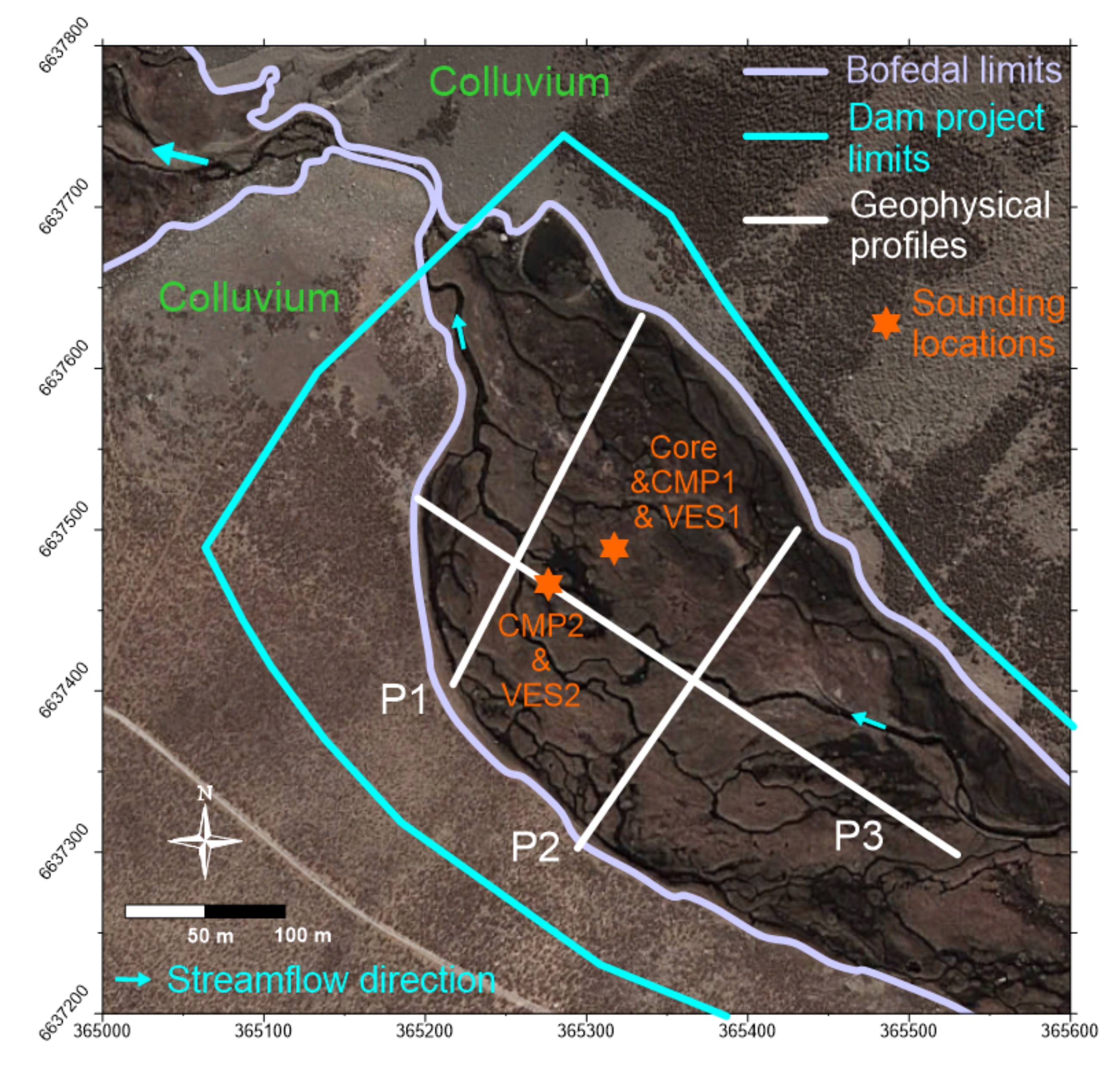
The fluvial plain from La Serena (Figure 1), which narrows toward the high Andes, is mainly composed of Quaternary alluvium of boulder, gravel, sand and clay, which forms the floor and marginal terraces of the Elqui Valley [43]. These lowlands are very suitable for growing crops, in comparison to the surrounding steep intrusive, volcanic, magmatic and volcano-sedimentary mountains. Agriculture is the primary economic activity outside of the combined La Serena–Coquimbo metropolitan area.

The agricultural area extends from the coast up to ~2000 m a.s.l. (Figure 1 and Figure 2). The first bofedales are observed above 2000 m a.s.l., where the protected area of the Estero Derecho Nature Sanctuary starts. The highest bofedal is detected at an elevation of 3750 m a.s.l., above which a glacial moraine prevents peat development. The sub-valley of Estero Derecho was chosen because there is a peatland network between these two limits, which was likely formed by the closure of the valley at various points due to the deposit of scree and colluvium from slopes and gullies above. This sub-valley is located between mountains that are mainly composed of magmatic rock, such as granites.

2.4. Study Site

The studied bofedal, called “Piuquenes”, was chosen due to its position in the central part of the existing bofedal range (3070 m; Figure 2) and its rounded-elongated shape which is representative of other bofedales in the region. The Estero Derecho River flows through the bofedal, exiting at the joining of two rock scree slopes that enable a small waterfall to form and mark the end of the studied bofedal. Further downstream the watercourse travels through other bofedal and rock scree systems. This bofedal, like many others in Estero Derecho, has been artificially widened using man-made canals to increase the vegetation available for cattle grazing. This peatland was also chosen because there is a proposal to create a dam at the bofedal outlet to improve control of water delivery for agricultural use. The boundaries of the proposed reservoir are shown in Figure 3.

The bofedal surface contrasts with its surroundings, having a darker colour associated with more vegetation than the surrounding terrain (Figure 3). While the bofedal surroundings consist of brownish sands and arid plants, such as cacti, the bofedal itself contains grass grazed by livestock and native biota. The main watercourse (arrows in Figure 3) and man-made canals cross the bofedal before converging and crossing the colluvium formations at the end of the bofedal. Around the peatland as well as on the steep slopes perpendicular to the river flow, the bedrock cannot be observed since it is covered by rock scree or colluvium and low arid vegetation.

3. Materials and Methods

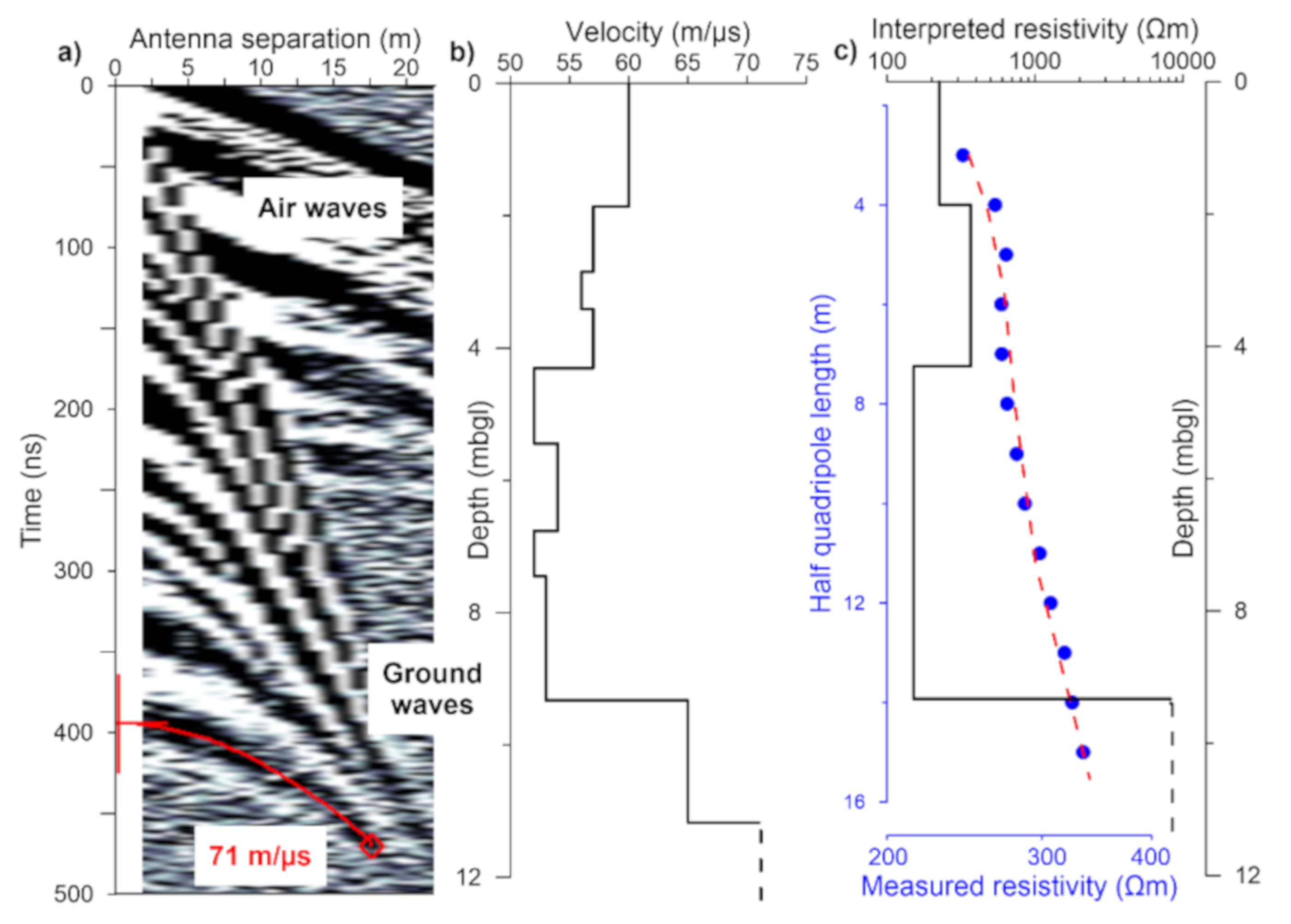
3.1. Vertical Electrical Sounding

Vertical Electrical Sounding (VES) and Electrical Resistivity Tomography (ERT) are geophysical methods that characterize the electrical resistivity distribution in the subsurface [44]. In this study, VES and ERT measurements were carried out during February 2019 using a TIGRE resistivity system and 32 stainless-steel electrodes. One resistivity measurement uses two dipoles: one dipole injecting current between two electrodes and one dipole measuring the potential difference between two other electrodes. The apparent electrical resistivity can then be calculated, depending on the electrode configuration [45]. Each measurement was repeated three times, and data were discarded if there was more than a 5% deviation between measurements. A Wenner–Schlumberger configuration was carried out with the measuring potential dipole at the centre of the current injecting dipole.

A VES consists of using a fixed measuring dipole, at the centre of the moving current dipole. The distance between the two electrodes of the current dipole and the electrical resistivity distribution define the depth to which the signal will penetrate. A larger distance results in a greater penetration depth. The sounding curve, made by plotting the apparent resistivity values together with the half-distance between the two current-electrodes, is then inverted in order to compute the 1D vertical resistivity model that best fits the data [45]. The software IPI2WIN was used to carry out the inversions [46].

3.2. Electrical Resistivity Tomography

ERT consists of various VES distributed along a profile line, which allows a 2D interpretation of the resistivity distribution [47]. ERT has been successfully used to locate laterally varying geology, such as fracture zones, and to discriminate soil from bedrock [48,49,50]. In this study, we used 32 electrode sets having the same inter-electrode distance (5 m) along a line together with the computer and the TIGRE switch box, which automatically use almost all of the Wenner–Schlumberger electrode configurations among the 32 electrodes. Three hundred and thirty-six quadripoles were used for the first two profiles using one roll-along procedure, whereas 630 quadripoles requiring three roll-along procedures that allow an extension of the profile length were used for the last profile. Positions were taken with a Trimble differential GPS to add topographical information to the ERT dataset. The inversion of apparent resistivity data was carried out with Res2dinv software (Geotomo Software; [51]), which provides 2D cross-sections of resistivity with a maximum depth of investigation in the range of 15 to 30 m, for the conditions of the present study. The larger the inter-electrode spacing, the deeper the investigation depth for similar acquisition and geological conditions. Nevertheless, it should be noted that with a conductive layer at shallow depth, such as a clay layer, the sensitivity of the model decreases substantially at depths greater than a few meters below the surface [48]. Electrical resistivity in peat soils mostly depends on pore fluid resistivity and the physical properties of the peat matrix, such as porosity, inorganic content and surface area [52]. Peat resistivity generally increases with depth when the mineral soil is a source of inorganic solutes for the peat pore water [24]. A significant contrast between peat and the underlying mineral soil will likely occur due to the markedly different physical characteristics of organic versus inorganic sediments [53]. Electrical resistivity depends on the water and clay content [50,54], as well as the media consolidation degree (

Table 1. Physical parameters relevant for the study of peatlands, extracted from [32,57,58,59,60].

Material	Electrical Resistivity (Ωm)	EM Wave Velocity (m/µs)
Ice	106–107	170
Water	10–100	30
Air	1014	300
Clay	1–100	47 (wet)–210 (dry)
Sand	100–5 × 103	54 (wet)–170 (dry)
Gravels	100–4 × 102	80–120
Granite	5 × 103–106	77 (wet and fractured)–130 (dry)
Peat	10–350	35–45

).

3.3. Ground Penetrating Radar

Similarly to the VES and ERT methods, Ground Penetrating Radar (GPR) uses a transmitter and a receiver. GPR differs from resistivity methods as it propagates a high frequency electro-magnetic (EM) wave through the transmitting antenna that is reflected at the boundary between materials with sufficiently different EM properties, such as geological discontinuities, and the receiving antenna measures the returned signal. The velocity of this EM wave is primarily controlled by the relative dielectric permittivity, a geophysical property strongly dependent on water content [32]. Measurements were taken with a Pulse Ekko system and a 50 MHz antenna and repeated 64 times to increase the signal-to-noise ratio. GPR can be used in two different modes, called Common Mid-Point (CMP) and Common Offset Profile (COP). CMP is similar to VES as it provides a 1D vertical sounding of the EM velocity by increasing the distance between the receiver and the transmitter centred on a CMP. The analyses of refraction hyperbolas contained in the CMP enable the calculation of the EM velocity [55]. EM velocity depends mainly on the water content (Table 1). COP were carried out with a fixed transmitter-receiver distance (2 m) and measurements were made along a line with a fixed step (0.66 and 1.14 m). COP allows a 2D interpretation of the reflectors, after a data post-process that consists mainly of adjusting gains, filters and a topographic correction [55]. Ekko-View software was used to process the data.

3.4. Core Extraction and Acquisition Strategy

One soil core of 1.3 m depth was extracted a year before the geophysical survey with a manual auger in the peatland (Figure 3). Samples were extracted from the ground every 25 cm and stored in PVC tubes. The sediment samples were interpreted and porosity estimations were completed by measuring dry and saturated sample weights with an accurate scale and comparing the calculated densities [56].

Three geophysical profiles and two soundings were acquired on the peatland (Figure 3). The first two profiles cross the bofedal more or less perpendicular to the valley, whereas the third profile is parallel to the river. This configuration allows a 3D interpretation of the peatland structure. The core as well as the first CMP and VES were acquired at the first sounding location, whereas the second CMP and VES were acquired on a relatively homogenous surface on the third profile.

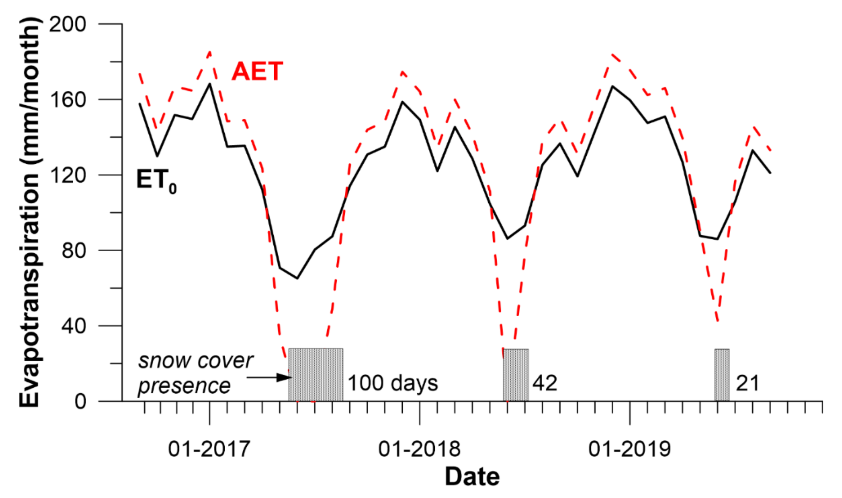
3.5. Evapotranspiration

The evapotranspiration was estimated using two automatic weather stations (AWS in Figure 1; www.ceazamet.cl). The AWS monitor wind velocity and direction, rainfall, air temperature and humidity. The northern station inside the Estero Derecho watershed (3020 m a.s.l.) has a snow height sensor, but no solar radiation sensor. Solar radiation from the nearest station (the southern AWS at 2500 m a.s.l.) was used to calculate the daily reference evapotranspiration ET₀. The latter is based on the formula given in [61], called the FAO Penman–Monteith. Derived from the well-known Penman–Monteith [62,63] equation; this reference evapotranspiration formula has proven its effectiveness in many locations and climates [61,64]. The actual evapotranspiration AET (mm) is calculated by multiplying ET₀ with the crop coefficients K_c (−) chosen from [61]. K_c values depend on land cover and plant stage.

3.6. Vegetation Cover Area

The satellite-derived vegetation index called Normalized Difference Vegetation Index (NDVI) has been used to assess the presence of live vegetation in satellite images for a number of decades [65]. Where the water table is shallow, the presence of live vegetation indicates the availability of groundwater during summer [65]. The NDVI temporal variability is a good indicator of vegetation variation in semi-arid areas [66]. The NDVI combines the spectral bands recorded by remote sensing satellites in a way that enhances the visibility of vegetation and reduces the visibility of other elements, such as soil, lighting and water. LandSat-8 products (30 m resolution) were used here to compute the NVDI. Field observation and satellite imagery were used to discriminate peatlands from crops.

4. Results

After the analysis of the geophysical results (soundings and cross-sections), a 3D computation of the alluvial filling identified with geophysics was carried out, before completing the hydrological interpretation of the bofedal water storage compared to other hydrological components (evapotranspiration, streamflow and precipitation).

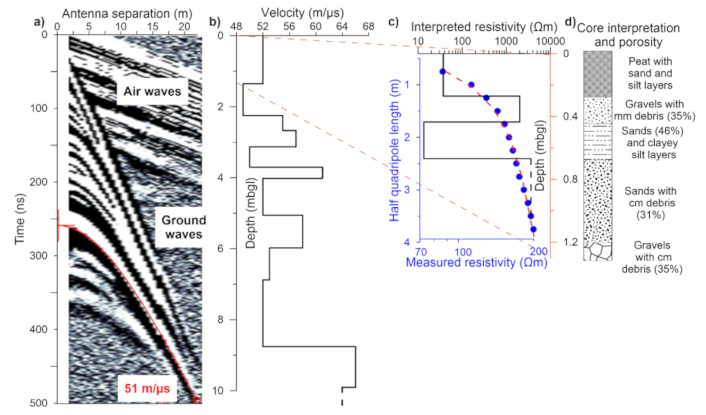
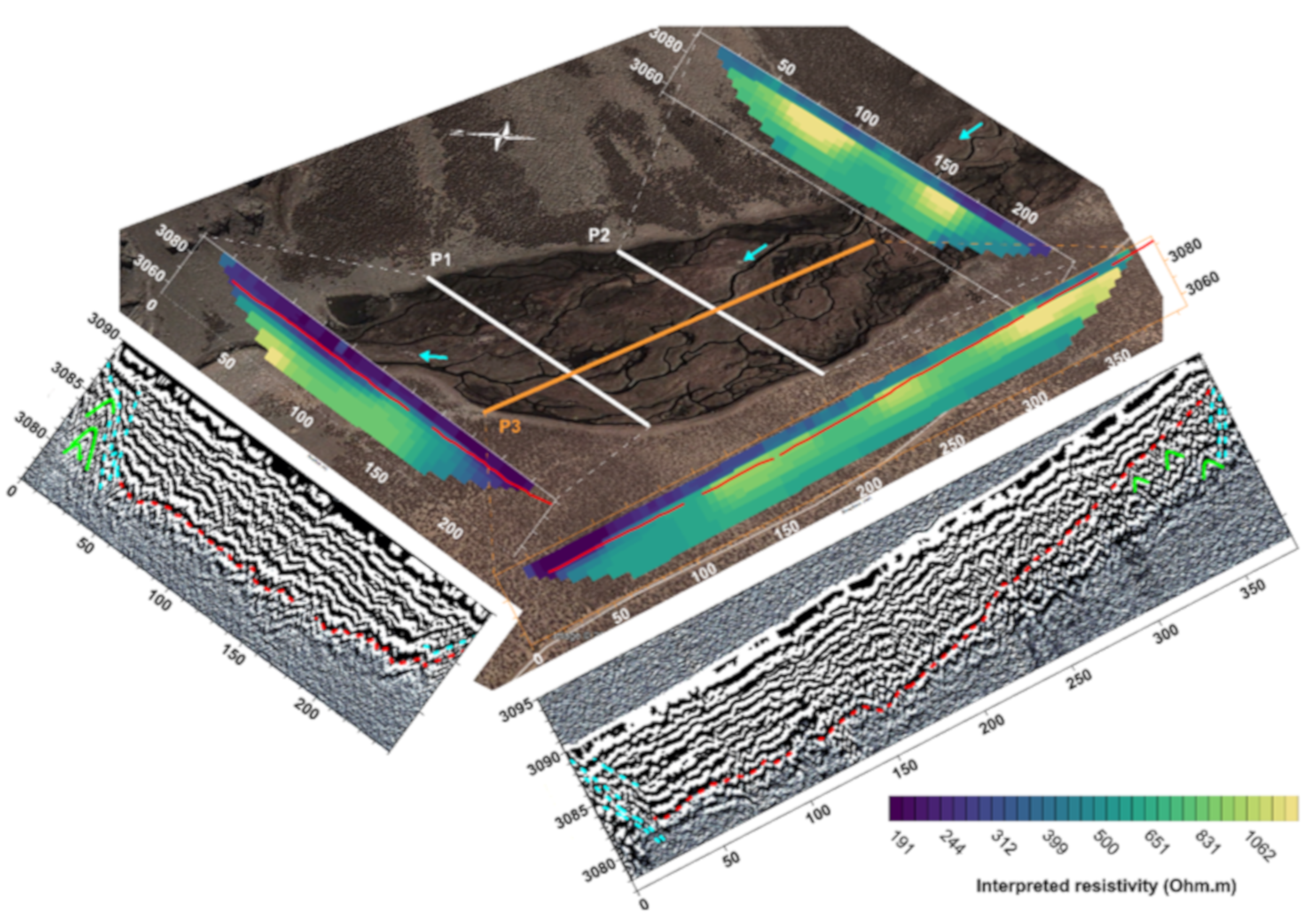
4.1. Geophysical Results

Raw data for each geophysical method at Sounding Location 1 are presented (Figure 4a for GPR in CMP mode, Figure 4c in blue for VES), as well as their interpreted models (Figure 4b for GPR, Figure 4c in black for VES). The GPR velocity model was calculated using the hyperbolas in the raw data, while the resistivity model was calibrated using the core interpretation (Figure 4d). Geophysical inversion processes generally face a non-uniqueness problem, meaning that several models can explain the data well [67]. The fit of the observed data with the output from the model is evaluated with a root mean square (RMS) error, which represents the square difference of the blue and red curves (Figure 4c). To avoid such non-uniqueness, a priori information can be used, such as core or geophysical information. In the case of Figure 4, using the a priori core thickness information led to a low RMS of 1.94%, which is an indicator of good model quality.

While the peat with coarse sand and silt layers, as well as the sand with clay-silt layers, are characterized by low resistivities below 40 Ωm, the clay-, silt- and peat-free layers, such as the gravels and sands, are marked by their high resistivity of more than 1000 Ωm (Figure 4c,d). The results are in agreement with Table 1, but are quite high for saturated gravels or sands values. This inconsistency could be linked to the non-uniqueness of the inversion process or to the high resistivity of pore water coming from snow or ice melt. The shallowest layer of the EM (GPR) velocity profile contains the four sediment layers observed in the VES and the core interpretations. The EM velocity corresponding to these four layers is 52 m/µs, which is in agreement with saturated peat, sand or clay (Table 1). The deeper GPR layer measured at a depth of 6–8.8 m should be composed of similar material because of the relatively low EM velocity variations (49 to 61 m µs^–1). Nonetheless, there are a significant number of GPR reflectors that may be interpreted as successive deposits of sediment layers, such as in the core. The two final reflectors at depths of 8.8 and 9.9 m display a sharper velocity contrast (52 to 66 m/µs) in comparison with the upper layers.

The second sounding is located at 100 m on P3 (Figure 3), where the peatland surface is relatively homogenous, so it was investigated using 1D methods. Similar to the first sounding, CMP2 is characterized by many reflectors (Figure 5a,b), but with slightly higher EM velocities (52 to 66 m/µs). There are also well-defined deeper reflectors with sharp velocity variations at depths of approximately 9.5 and 11 m. Those layers are characterized by their higher EM velocities of 65 and 71 m/µs. The VES model contains a priori thickness information from GPR models. Various tests were carried out in order to obtain a low RMS value, a limited layers number and fixed thicknesses from the velocity model. The first three layers have resistivities between 150 and 400 Ωm, which contrast less than the layers at Sounding Location 1. This low contrast can largely be explained by the dipole spacing, as the spacing between each electrode at Sounding Location 1 was 0.25 cm, while for Location 2 it was 1 m. The resolution is therefore much lower for Location 2, resulting in reduced sensitivity and ability to detect variations in resistivity associated with thinner layers. Velocities and resistivities of the first 9.5 m are in agreement with values in Table 1 for sands and gravels mixed with some thin clay or silt layers, as observed in the core. Higher EM velocities seem to be linked to higher resistivities, as observed in the upper layers (Figure 4 and Figure 5), but this is not always the case as, for example, the second layer in Figure 5 (from 2 to 4 m depth, approximatively). This might be a gravel layer with some thin clay or peat beds. The third resistivity layer in Figure 5 (from 4 to 9 m depth, approximatively) reaffirms the positive correlation between velocities and resistivities as it has the lowest resistivity and velocity values observed. This layer should contain peat or clays until a depth of 9.5 m. At this depth there is a sharp shift toward very high resistivity and relatively high velocity values (Figure 5b,c). This shift could be explained by an unconsolidated clay-free material (low EM velocity in Table 1) with low water content (high resistivity), such as boulders or rock scree colluvium.

The results of the three profiles are presented in Figure 6, where the ERT and GPR cross-sections allow an investigation depth of about 30 m and 10 m, respectively. The vertical scale of the GPR sections is exaggerated (7 times) in order to properly display the reflectors. In order to transform the GPR time scale into a depth scale, averaged EM velocities derived from the CMPs were used. The 10th reflector near the CMP2 location (Figure 5) is highlighted in red (Figure 6), since it should correspond to the sharp EM velocity variation observed in CMP2. Assuming this reflector represents the base of the bofedal, the maximum thickness is about 10 m, reducing upstream to a depth of 4 m (end of P3). The red reflector of the transverse profile (P1) displays a relatively constant thickness across the bofedal. This reflector ends near the sub-vertical (NE of P1, NW of P3), interpreted as colluvium slopes covered with alluvium. Beneath these reflectors, there are indeed diffraction hyperbolas (green lines in Figure 6), interpreted as boulders or rock scree. The CMPs (Figure 4 and Figure 5) and the GPR profiles (Figure 6) show various sub-horizontal reflectors above the reflector highlighted with a red line, interpreted as sediment layers with distinct EM properties.

The red GPR reflector, representing the bofedal base, is also displayed on the ERT cross-sections to improve the interpretation. These reflectors are in agreement with the ERT results, as they separate two zones with contrasting resistivities. The shallowest zone is relatively conductive with resistivities between 150 and 600 Ωm, whereas below the red reflector higher resistivities are observed from 500 to 1500 Ωm. The shallow conductive zone is thicker and more conductive downstream than upstream, observed along line P3 and confirmed at P2. We expect that the conductive zone is made up of thinner alluvial material (sands, silts), as seen in the core (Figure 4). The geomorphological interpretation of these results is discussed in Section 5.

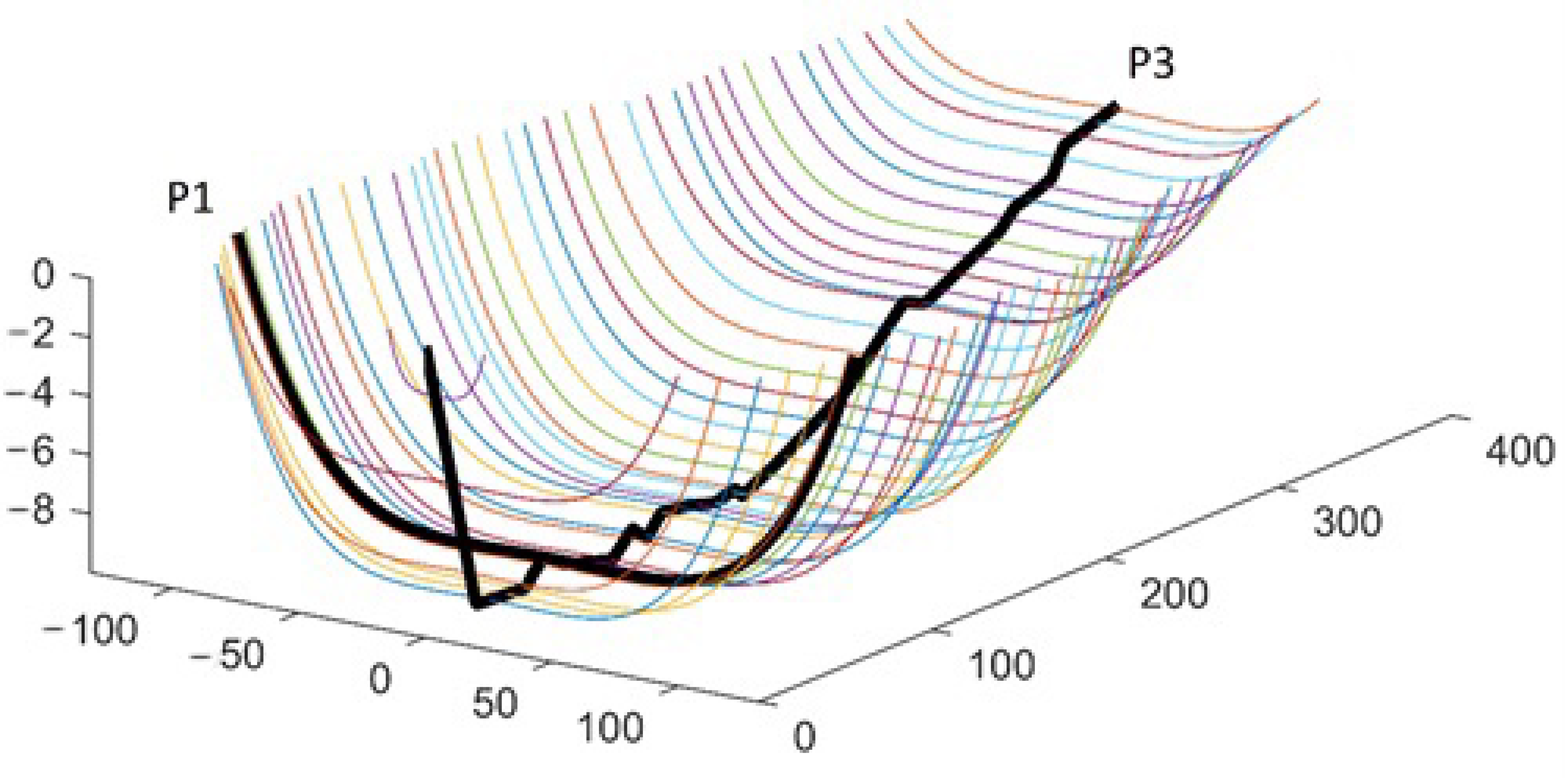
4.2. Water Storage Capacity Assessment

The water storage capacity of the alluvial deposits within the bofedal can be assessed using the geophysical results and the porosity measurements. In order to compute the 3D volume of the alluvial filling, one should delineate the bofedal surface area, its lateral limits and its lower limit. While the surface area can be delineated using satellite imagery (Figure 3), its lower and lateral limits need to be interpolated using the geophysical data. To that end several assumptions are required:

(1)

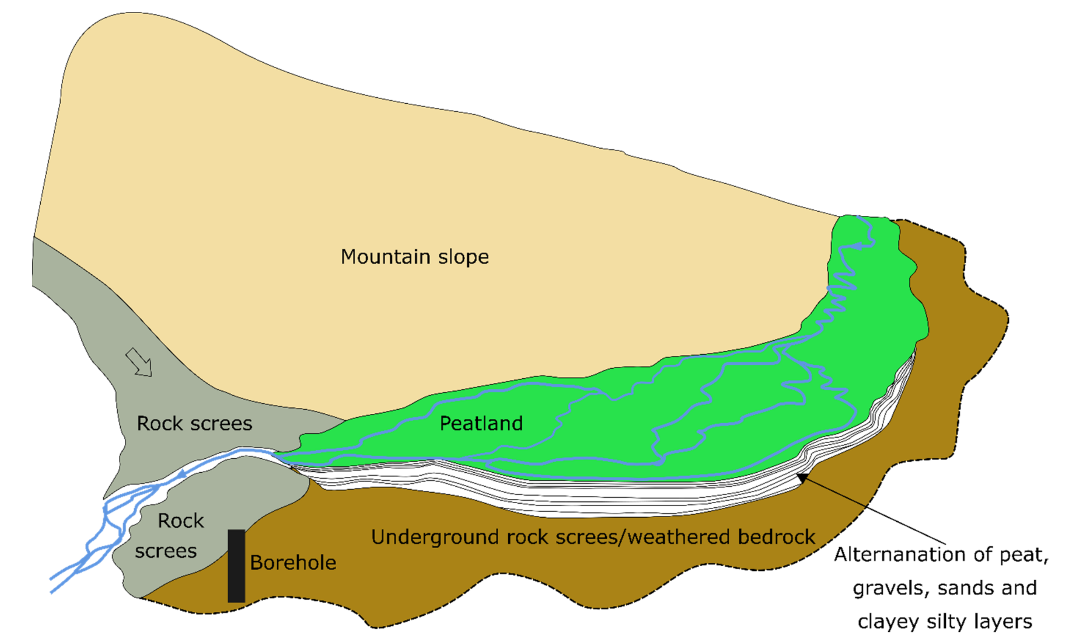
That the lateral limits of the bofedal identified in the GPR sections (dashed blue lines in Figure 6) mark the end of the filling. It is expected from a geomorphological perspective that the alluvial filling would not develop beneath the colluvium. This idea is supported by hyperbolas observed below the lateral limit on line P1 (Figure 6), which are interpreted as boulder or rock scree, marking the end of the alluvial deposits.

(2)

The deep red reflectors (observed in profiles P1 and P3 in Figure 6) represent the maximum depth of the alluvial deposits perpendicular to the longitudinal P3 profile. From the P1 GPR section, it can be seen that this reflector has approximately a constant elevation of ~3081 m a.s.l.

(3)

That the filling is symmetrically distributed perpendicular to the longitudinal profile P3 (Figure 6 and Figure 7). This assumption is supported by the P1 and P2 profiles, which show some symmetry.

Applying these assumptions, symmetrical 4th order polynomials were used to extrapolate the filling’s lower limit perpendicular to P3 at one meter spacing (Figure 7), constrained by the two lateral limits at the bofedal surface and the maximum depth in the middle of the profile. The polynomial was calibrated using the P1 profile since the lower limit of the filling can be estimated well with the P1 red reflector (Figure 6), resulting in an RMSE error of 0.53 m.

The alluvial filling volume is estimated to be 530,000 m³ for the area studied with geophysics, which contains the bofedal surface from the peatland outlet to the southeast side of P3 (Figure 3). By extrapolating the upstream bottom curve until the extension of the projected dam reservoir (Figure 3), we obtain a filling volume of 600,000 m³ for the dam extension. Assuming that the filling is composed of gravels and sands with debris or clay-silt beds, as in the core, and by taking the median porosity (35%) of the four measurements, the water storage capacity is about 185,000 to 210,000 m³, for the study area and the dam extension, respectively. If the minimum (31%) and maximum porosity (46%) are applied, the water storage capacities are 164,000 to 243,000 m³ for the study area and 186,000 to 276,000 m³ for the dam extension. In comparison to the usable volume of the projected reservoir of 1,600,000 m³ [68], the natural storage capacity of the bofedal is about 13% (11.6 to 17.3%) of the future dam capacity. The storage capacity of the bofedal relative to the dam increases if the deterioration of downstream peatlands due to the dam creation and the flow restriction is taken into account. We only consider the water content capacity of the alluvial filling and not the water content in the more consolidated basal material.

A basic computation of the reservoir capacity was completed using the water volume of 185,000 m³ and the studied bofedal surface (about 0.09 km²), leading to a reserve of approximately 2000 mm (1770 to 2630 mm) of water per square meter of bofedal.

4.3. Evapotranspiration Estimates

Water losses through evapotranspiration from vegetated areas were estimated for the Estero Derecho catchment in order to determine if these losses are significant relative to the average precipitation and runoff. Because vegetation is usually covered by snow in winter, evapotranspiration should be rather limited, while during the rest of the year plants will be exposed to air and able to evapotranspire. Snow presence was derived from the AWS in the Estero Derecho catchment (Figure 1) using a snow height sensor. When snow was present, we assumed no evapotranspiration from plants and soils (K_c = 0), while a value of 1.1 for K_c,, based on wetland values in [61], was used for the remaining period (Figure 8). Peatland actual evapotranspiration (AET) was calculated from ET₀ and K_c. There is a clear seasonal trend with lower ET₀ and AET in winter than in summer (Figure 8).

The annual AET values (from May to April) as well as the peatland water storage capacity from the previous section are reported in the first two columns of

Table 2. Annual AET values and water storage capacity (stock) at the peatland and watershed scales, streamflow presented as water height (mm) and precipitation (precip) corresponding to rain gauge data downstream of the Estero Derecho catchment (Figure 1).

	Peatland Scale (mm)		Watershed Scale (mm)			Precip in Horcon (mm)
	Peatland Annual AET	Peatland Stock	Peatlands Annual AET	Peatlands Stock	Stream Flow
2017–2018	1520	2000	35.1	46.2	103	240
2018–2019	1660		38.3		54	33

. These values were extrapolated to the green areas at the watershed scale using the NVDI and aerial photography in the gauged portion of Estero Derecho (Figure 1). Vegetation covers 3.08% of the gauged catchment. Agriculture accounts for about 25% of the cover, while peatlands make up the other 75%. Thus, peatlands AET and stocks can be computed at the watershed scale by multiplying the peatland scale results by the peatland cover ratio (3.08% × 75%). This analysis assumes that the other peatlands have a similar depth and structure, such that the reserve is consistently 2000 mm of water per square meter of bofedal. Peatland AET and stocks are higher than annual precipitation at the watershed scale during the driest year (2018–2019), as shown in Table 2. They are also in the same order of magnitude as the annual streamflow (Table 2) at the outlet of the Estero Derecho watershed during 2018–2019 (Figure 1). The hydrological system of peatlands is discussed in the next section.

5. Discussion

In this section we discuss the geomorphological interpretation of the “Piuquenes” Bofedal, then the hydrological role and functioning of high-altitude peatlands.

5.1. Bofedal Geomorphological Interpretation

Rock scree appears to play a major role in the bofedal formation, restricting water flow and thus aiding the creation of a basin bofedal (Figure 9). According to the classification of [4], this bofedal is a basin peatland. The barrier created by rock scree allows alluvial deposits to accumulate at the barrier and then progressively upstream. The latter is supported by the basin-shape and the thicker material downstream compared to upstream derived from the geophysical analysis. The numerous reflectors, the low resistivity and the depth of the sharp resistivity and GPR velocity contrast point towards such an interpretation.

The alluvial layers which are likely composed of peat, sand, gravel and clay materials are limited at depth by a material composed of rock scree or weathered granite bedrock. This interpretation is supported by the relatively high resistivity and velocities at depth, as well as by a geotechnical study carried out for dam construction that has been proposed for development on the studied bofedal [68]. Low seismic velocities at depth (2000 ms⁻¹) were found in the middle of the peatland, while high velocities (4000 ms⁻¹) were detected on the mountain slope side (NE). Those high velocities are typical for a consolidated unweathered granite, whereas the low velocities are most likely a transition material between sedimentary layers and consolidate media. Boreholes drilled in the frontal rock scree until a depth of 60 m and on the mountain slope at the SW side of the bofedal, contained rock scree with a sandy matrix and no evidence of bedrock [68].

5.2. Hydrological Role of High-Altitude Peatlands

Bofedales in north-central Chile are located between the upstream cryosphere reserve (snow and ice) and downstream agricultural production and human-needs areas. They contribute water downstream, but also lose a significant amount of water through evapotranspiration (Section 4.3; Table 2). The amount of evapotranspiration could be negatively correlated to the water table depth, as shown by [69]. Hence, despite the seasonal trend observed at a regional scale, with the shallowest groundwater levels observed during summer time and deepest groundwater levels observed during wintertime, groundwater levels in Andean wetlands behave inversely as they are influenced by evapotranspiration cycles [70]. Peatland drainage can have a significant role in lowering the water table [71].

Bofedales act as important water reservoirs at the watershed scale because their water storage is on the same order of magnitude as the streamflow and can be higher than the annual precipitation (Table 2), as seen in Section 4.2 and Section 4.3. While sands and gravels, which have a high potential for water circulation, make up much of the alluvial deposits within the “Piuquenes” bofedal, vertical fluxes are likely to be very slow due to the presence of thin layers of clay and silt. Ice layers were observed in the winter, and these could also inhibit the vertical flow of water. Whilst pronounced vertical gradients were found in a basin peatland [72], other studies have observed low permeability ratio values (horizontal to vertical permeability ratio) of ~100 or 1000 m²/m² in peatlands [73,74]. Mineral layers in peatlands, such as sub-horizontal clay deposits, can also restrict vertical groundwater exchanges [75]. Restricted vertical fluxes, such as deep infiltration, implies that bofedales have the potential to hold water for a long period which could prove useful during droughts.

During the mega drought from 2009 to 2015 [76], streamflows in the region were very low (Figure 10), and the downstream reservoir was almost empty in 2014. This mega drought was characterized by six consecutive years of precipitation below the average with negative consequences on water resources availability. Annual minimum specific discharge (discharge per unit area of watershed) were extracted at the outlets of Estero Derecho and its neighbouring catchment, Cochiguaz (Figure 1), in order to assess the bofedales’ role during low streamflow stages. These low stages are assumed to represent catchment baseflow. These two catchments, which together form the Rio Claro watershed, are ideal for comparison since they have the same climatic, geographic and geological conditions. They are composed of incised valleys surrounded by plutonic rocks of similar elevations in the same semi-arid climate [43]. The main differences are the size (785 vs. 393 km²) and vegetation cover ratio (1.16% vs. 3.08%) for the Cochiguaz vs. Estero Derecho catchments. The minimum specific discharge measured in Cochiguaz is generally higher than Estero Derecho (Figure 10), which could be explained by the higher vegetated coverage of Estero Derecho compared to Cochiguaz (12.1 vs. 9.11 km²), which consumes more water through evapotranspiration. Higher precipitation or larger aquifers maintaining a higher baseflow in Cochiguaz could also explain this difference, but there is no evidence supporting these hypotheses. In fact, the Cochiguaz watershed has a lower mean elevation than Estero Derecho (3511 vs. 3544 m a.s.l.), and it likely receives less precipitation [77].

The difference between the minimum specific streamflow of the two watersheds tends towards zero at the end of the mega drought (Figure 10, years 2014 and 2015). Moreover, the Estero Derecho minimum streamflow displays a lower temporal variability than Cochiguaz, which could be explained by a more stable baseflow in Estero Derecho than Cochiguaz. Such a baseflow could be maintained by rock glaciers or bofedales. This explanation is reasonable since rock glacier and bofedal cover ratios are higher in Estero Derecho than in Cochiguaz (7.88% vs. 4.91% for the rock glacier cover ratios, respectively).

Future research should further investigate recharge processes of mountain peatlands and their contributions to regional hydrological systems. Isotopic analysis should be the next step in order to better characterize the hydrological functioning. Evaluation of groundwater or snowmelt contribution to streamflow is recommended [78,79]. These altitude peatlands are not only water consuming reservoirs, but also allow for mixing of water from different origins, such as the main water course, small mountain streams and groundwater from several sources [36,69]. The important role of hillslope subsurface flow for peatland recharge and streamflow generation should be assessed, as demonstrated in other Andean peatlands [80]. Future research should also focus on factors playing an important role in the circulation of water and changes in the water level, by using a statistical approach such as [81] and [82], in order to discriminate the effects of slope, altitude, climate, hydrology and peatland underground structure.

6. Conclusions

The combination of ERT and GPR geophysical methods enable a better understanding of both the geological composition and the geometry of high-altitude peatlands. According to these results, and to the extracted core data, the studied bofedal is composed of layers of saturated unconsolidated sediments with a low clay content, such as sands, gravels and silts beds. Those layers are expected to be found until a depth of approximately 10 m, where a strong contrast in resistivity and EM velocity marks the limit between the bottom of the alluvial filling and the top of a media probably composed of rock scree or weathered bedrock, inferred from the high resistivity and relatively high EM velocities.

By carrying out longitudinal and transversal profiles and following the strong resistivity and velocity interface, it was possible to define the bofedal geometry as a basin-shaped landform, with thicker sediment filling downstream than upstream. Converging rock scree lobes form a barrier that defines the downstream limit of the bofedal. Together, these observations suggest that the bofedal was formed by the closing of the valley by scree, and the progressive deposition of alluvial deposits upstream.

The water storage capacity of this alluvial filled structure is estimated to be 2000 mm per square meter of bofedal, which translates to a reservoir capacity comparable to the annual streamflow and the actual peatland evapotranspiration at the basin scale. Thus, high-altitude peatlands (bofedales) are important water reservoirs that consume a significant amount of water in arid environments, but are necessary to provide the essential eco-services of peat, soil, plant production and carbon accumulation. Thanks to their reservoir function and their low vertical permeability, bofedales may buffer the impact of droughts. Efforts to characterize the hydrological role of and preserve these unique wetlands critical for sustaining biodiversity and livestock grazing must be a priority in the context of a changing climate.

References

1. De Carolis Friedmann, G. Descripción del Sistema Ganadero y Hábitos Alimentarios de Camélidos Domésticos y Ovinos en el Bofedal de Parinacota; Universidad de Chile: Santiago, Chile, 1987. [Google Scholar]
2. Moreau, S.; Bosseno, R.; Gu, X.F.; Baret, F. Assessing the biomass dynamics of Andean bofedal and totora high-protein wetland grasses from NOAA/AVHRR. Remote Sens. Environ. 2003, 85, 516–529. [Google Scholar] [CrossRef]
3. Coronel, J.S.; Declerck, S.; Maldonado, M.; Ollevier, F.; Brendonck, L. Temporary shallow pools in high-Andes “bofedal” peatlands: A limnological characterization at different spatial scales. Arch. des Sci. 2004, 57, 85–96. [Google Scholar]
4. Squeo, F.A.; Warner, B.G.; Aravena, R.; Espinoza, D. Bofedales: High Altitude Peatlands of the Central Andes Bofedales: Turberas de Alta Montaña de los Andes Centrales. Rev. Chil. Hist. Nat. 2006, 79, 245–255. [Google Scholar]
5. Chimner, R.A.; Lemly, J.M.; Cooper, D.J. Mountain fen distribution, types and restoration priorities, San Juan Mountains, Colorado, USA. Wetlands 2010, 30, 763–771. [Google Scholar] [CrossRef]
6. Comas, X.; Terry, N.; Hribljan, J.A.; Lilleskov, E.A.; Suarez, E.; Chimner, R.A.; Kolka, R.K. Estimating belowground carbon stocks in peatlands of the Ecuadorian páramo using ground-penetrating radar (GPR). J. Geophys. Res. Biogeosci. 2017, 122, 370–386. [Google Scholar] [CrossRef]
7. Li, Z.; Gao, P.; You, Y. Characterizing Hydrological Connectivity of Artificial Ditches in Zoige Peatlands of Qinghai-Tibet Plateau. Water 2018, 10, 1364. [Google Scholar] [CrossRef] [Green Version]
8. Van Damme, P. Disponibilidad, uso y Calidad de los Recursos Hídricos en Bolivia; Cumbre Mundial sobre el Desarrollo Sostenible: Johannesburg, South Africa, 2002. [Google Scholar]
9. Earle, L.R.; Warner, B.G.; Aravena, R. Rapid development of an unusual peat-accumulating ecosystem in the Chilean Altiplano. Quat. Res. 2003, 59, 2–11. [Google Scholar] [CrossRef]
10. Reboratti, C. La situacion ambiental en las ecoregiones Puna y Altos Andes. In La Situación Ambiental Argentina 2005; Brown, A., Martinez Ortiz, U., Acerbi, M., Corcuera, J., Eds.; Fundación Vida Silvestre Argentina: Buenos Aires, Argentina, 2006; p. 577. ISBN 9509427144. [Google Scholar]
11. Wright, A.C.S. Los bofedales-alkaline cushion-peatland peats of the semi-arid Chilean Altiplano. Pac. Viewp. 1962, 4, 189–193. [Google Scholar] [CrossRef]
12. Alzérreca, H.; Prieto, G.; Laura, J.; Luna, D.; Laguna, S. Características y Distribución de los Bofedales en el Ámbito Boliviano; Editorial Plural Editores: La Paz, Bolivia, 2001. [Google Scholar]
13. Fonkén, M.S.M. An introduction to the bofedales of the Peruvian High Andes. Mires Peat 2014, 15, 1–13. [Google Scholar]
14. Otto, M.; Scherer, D.; Richters, J. Hydrological differentiation and spatial distribution of high altitude wetlands in a semi-arid Andean region derived from satellite data. Hydrol. Earth Syst. Sci. Discuss. 2011, 8, 1287–1327. [Google Scholar] [CrossRef]
15. Scott, D.A.; Carbonell, M. A Directory of Neotropical Wetlands; IUCN Conservation Monitoring Centre: Cambridge, UK, 1986. [Google Scholar]
16. Clymo, R.S. The Limits to Peat Bog Growth. Philos. Trans. R. Soc. B Biol. Sci. 1984, 303, 605–654. [Google Scholar]
17. Crum, H.; Planisek, S. A Focus on Peatlands and Peat Mosses, 1st ed.; University of Michigan Press: Ann Arbor, MT, USA, 1992. [Google Scholar]
18. Moore, P.D. The ecology of peat-forming processes: A review. Int. J. Coal Geol. 1989, 12, 89–103. [Google Scholar] [CrossRef]
19. Gorham, E. Northern Peatlands: Role in the Carbon Cycle and Probable Responses to Climatic Warming. Ecol. Appl. 1991, 1, 182–195. [Google Scholar] [CrossRef] [PubMed]
20. Maimer, N. Peat accumulation and the global carbon cycle. In Greenhouse-Impact on Cold-Climate Ecosystems and Landscapes; Boer, M., Koster, E., Eds.; Catena: Reiskirchent, Germany, 1992; Volume 22, p. 151. ISBN 9783923381319. [Google Scholar]
21. Belyea, L.R.; Baird, A.J. Beyond “the limits to peat bog growth”: Cross-scale feedback in peatland development. Ecol. Monogr. 2006, 76, 299–322. [Google Scholar] [CrossRef]
22. Ruthsatz, B. Flora und ökologische Bedingungen hochandiner Moore Chiles zwischen 18°00’ (Arica) und 40°30’ (Osorno) südl. Br. Phytocoenologia 1993, 23, 157–199. [Google Scholar] [CrossRef]
23. Wilcox, B.P.; Bryant, F.C.; Wester, D.; Allen, B.L. Grassland communities and soils on a high elevation grassland of central Peru. Phytologia 1986, 61, 231–250. [Google Scholar]
24. Slater, L.D.; Reeve, A. Investigating peatland stratigraphy and hydrogeology using integrated electrical geophysics. Geophysics 2002, 67, 365–378. [Google Scholar] [CrossRef] [Green Version]
25. Lowe, D.J. Application of impulse radar to continuous profiling of tephra-bearing lake sediments and peats: An initial evaluation. N. Z. J. Geol. Geophys. 1985, 28, 667–674. [Google Scholar] [CrossRef] [Green Version]
26. Pelletier, R.E.; Davis, J.L.; Rossiter, J.R. Peat analyses in the Hudson Bay Lowlands using ground penetrating radar. In IGARSS ‘91, Proceedings of the 11th Annual International Geoscience and Remote Sensing Symposium, Espoo, Finland, 3–6 June 1991; Institute of Electrical and Electronics Engineers, Inc.: New York, NY, USA, 1991; Volume 4, pp. 2141–2144. [Google Scholar]
27. Meyer, J.H. Investigation of Holocene organic sediments—A geophysical approach. Int. Peat J. 1989, 3, 45–57. [Google Scholar]
28. Comas, X.; Slater, L.; Reeve, A. Geophysical evidence for peat basin morphology and stratigraphic controls on vegetation observed in a Northern Peatland. J. Hydrol. 2004, 295, 173–184. [Google Scholar] [CrossRef]
29. Slater, L.; Comas, X.; Ntarlagiannis, D.; Moulik, M.R. Resistivity-based monitoring of biogenic gases in peat soils. Water Resour. Res. 2007, 43, 10. [Google Scholar] [CrossRef] [Green Version]
30. Kettridge, N.; Comas, X.; Baird, A.; Slater, L.; Strack, M.; Thompson, D.; Jol, H.; Binley, A. Ecohydrologically important subsurface structures in peatlands revealed by ground-penetrating radar and complex conductivity surveys. J. Geophys. Res. Biogeosci. 2008, 113, G4. [Google Scholar] [CrossRef] [Green Version]
31. Sass, O.; Friedmann, A.; Haselwanter, G.; Wetzel, K.F. Investigating thickness and internal structure of alpine mires using conventional and geophysical techniques. Catena 2010, 80, 195–203. [Google Scholar] [CrossRef]
32. Comas, X.; Terry, N.; Slater, L.; Warren, M.; Kolka, R.; Kristiyono, A.; Sudiana, N.; Nurjaman, D.; Darusman, T. Imaging tropical peatlands in Indonesia using ground-penetrating radar (GPR) and electrical resistivity imaging (ERI): Implications for carbon stock estimates and peat soil characterization. Biogeosciences 2015, 12, 2995–3007. [Google Scholar] [CrossRef] [Green Version]
33. Sjöberg, Y.; Marklund, P.; Pettersson, R.; Lyon, S.W. Geophysical mapping of palsa peatland permafrost. Cryosphere 2015, 9, 465–478. [Google Scholar] [CrossRef] [Green Version]
34. Yáñez, G.A.; Ranero, C.R.; von Huene, R.; Díaz, J. Magnetic anomaly interpretation across the southern central Andes (32°-34° S): The role of the Juan Fernández Ridge in the late Tertiary evolution of the margin. J. Geophys. Res. Solid Earth 2001, 106, 6325–6345. [Google Scholar] [CrossRef]
35. Favier, V.; Falvey, M.; Rabatel, A.; Praderio, E.; López, D. Interpreting discrepancies between discharge and precipitation in high-altitude area of chile’s norte chico region (263–2° S). Water Resour. Res. 2009, 45, 1–20. [Google Scholar] [CrossRef] [Green Version]
36. Valois, R.; MacDonell, S.; Núñez Cobo, J.H.; Maureira-Cortés, H. Groundwater level trends and recharge event characterization using historical observed data in semi-arid Chile. Hydrol. Sci. J. 2020. [Google Scholar] [CrossRef]
37. Núñez, J.; Rivera, D.; Oyarzún, R.; Arumí, J.L. Influence of Pacific Ocean multidecadal variability on the distributional properties of hydrological variables in north-central Chile. J. Hydrol. 2013, 501, 227–240. [Google Scholar] [CrossRef]
38. Réveillet, M.; MacDonell, S.; Gascoin, S.; Kinnard, C.; Lhermitte, S.; Schaffer, N. Uncertainties in the spatial distribution of snow sublimation in the semi-arid Andes of Chile. Cryosph. Discuss. 2019, 1–34. [Google Scholar] [CrossRef] [Green Version]
39. Sproles, E.A.; Kerr, T.; Orrego Nelson, C.; Lopez Aspe, D. Developing a Snowmelt Forecast Model in the Absence of Field Data. Water Resour. Manag. 2016, 30, 2581–2590. [Google Scholar] [CrossRef]
40. Gascoin, S.; Kinnard, C.; Ponce, R.; Lhermitte, S.; MacDonell, S.; Rabatel, A. Glacier contribution to streamflow in two headwaters of the Huasco River, Dry Andes of Chile. Cryosphere 2011, 5, 1099–1113. [Google Scholar] [CrossRef] [Green Version]
41. Perucca, L.; Angillieri, E. Glaciers and rock glaciers’ distribution at 28° SL, Dry Andes of Argentina, and some considerations about their hydrological significance. Environ. Earth Sci. 2011, 64, 2079–2089. [Google Scholar] [CrossRef]
42. Schaffer, N.; MacDonell, S.; Réveillet, M.; Yáñez, E.; Valois, R. Rock glaciers as a water resource in a changing climate in the semiarid Chilean Andes. Reg. Environ. Chang. 2019, 1–17. [Google Scholar] [CrossRef]
43. Jones, P.H. Geology and ground-water conditions in the lower valley of the Rio Elqui of Chile. Econ. Geol. 1953, 48, 457–491. [Google Scholar] [CrossRef]
44. Dahlin, T. The development of DC resistivity imaging techniques. Comput. Geosci. 2001, 27, 1019–1029. [Google Scholar] [CrossRef] [Green Version]
45. Zohdy, A.A.R. A new method for the automatic interpretation of Schlumberger and Wenner sounding curves. Geophysics 1989, 54, 245–253. [Google Scholar] [CrossRef]
46. Bobachev, C. IPI2Win: A windows software for an automatic interpretation of resistivity sounding data. Moscow State Univ. 2002, 320. [Google Scholar]
47. Greggio, N.; Giambastiani, B.; Balugani, E.; Amaini, C.; Antonellini, M. High-Resolution Electrical Resistivity Tomography (ERT) to Characterize the Spatial Extension of Freshwater Lenses in a Salinized Coastal Aquifer. Water 2018, 10, 1067. [Google Scholar] [CrossRef] [Green Version]
48. Valois, R.; Camerlynck, C.; Dhemaied, A.; Guerin, R.; Hovhannissian, G.; Plagnes, V.; Rejiba, F.; Robain, H. Assessment of doline geometry using geophysics on the Quercy plateau karst (South France). Earth Surf. Process. Landf. 2011, 36, 1183–1192. [Google Scholar] [CrossRef]
49. Valois, R.; Galibert, P.Y.; Guerin, R.; Plagnes, V. Application of combined time-lapse seismic refraction and electrical resistivity tomography to the analysis of infiltration and dissolution processes in the epikarst of the Causse du Larzac (France). Near Surf. Geophys. 2016, 14, 13–22. [Google Scholar] [CrossRef]
50. Valois, R.; Cousquer, Y.; Schmutz, M.; Pryet, A.; Delbart, C.; Dupuy, A. Characterizing Stream-Aquifer Exchanges with Self-Potential Measurements. Groundwater 2018, 56, 437–450. [Google Scholar] [CrossRef] [PubMed]
51. Loke, M.H.; Barker, R.D. Rapid least-squares inversion of apparent resistivity pseudosections by a quasi-Newton method1. Geophys. Prospect. 1996, 44, 131–152. [Google Scholar] [CrossRef]
52. Theimer, B.D.; Nobes, D.C.; Warner, B.G. A study of the geoelectrical properties of peatlands and their influence on ground-penetrating radar surveying. Geophys. Prospect. 1994, 42, 179–209. [Google Scholar] [CrossRef]
53. Comas, X.; Slater, L.; Reeve, A.S. Pool patterning in a northern peatland: Geophysical evidence for the role of postglacial landforms. J. Hydrol. 2011, 399, 173–184. [Google Scholar] [CrossRef]
54. Vouillamoz, J.M.; Valois, R.; Lun, S.; Caron, D.; Arnout, L. Can groundwater secure drinking-water supply and supplementary irrigation in new settlements of North-West Cambodia? Hydrogeol. J. 2016, 24, 195–209. [Google Scholar] [CrossRef] [Green Version]
55. Neal, A. Ground-penetrating radar and its use in sedimentology: Principles, problems and progress. Earth-Science Rev. 2004, 66, 261–330. [Google Scholar] [CrossRef]
56. Hao, X.; Ball, B.C.; Culley, J.L.B.; Carter, M.R.; Parkin, G.W. Soil Density and Porosity. In Soil Sampling and Methods of Analysis; Carter, M.R., Gregorich, E.G., Eds.; Canadian Society of Soil Science: Pinawa, MB, Canada, 2008; p. 1261. ISBN 9780849335860. [Google Scholar]
57. Jol, H. Ground Penetrating Radar Theory and Applications; Elsevier: Amsterdam, The Netherlands, 2009; ISBN 9780444533487. [Google Scholar]
58. Asadi, A.; Huat, B.B.K. Electrical resistivity of tropical peat. Electron. J. Geotech. Eng. 2009, 14 P, 1–9. [Google Scholar]
59. Maurer, H.; Hauck, C. Instruments and methods: Geophysical imaging of alpine rock glaciers. J. Glaciol. 2007, 53, 110–120. [Google Scholar] [CrossRef] [Green Version]
60. Parry, L.E.; West, L.J.; Holden, J.; Chapman, P.J. Evaluating approaches for estimating peat depth. J. Geophys. Res. Biogeosciences 2014, 119, 567–576. [Google Scholar] [CrossRef]
61. Allen, R.; Pereira, L.; Raes, D.; Smith, M. Crop. Evapotranspiration—Guidelines for Computing Crop Water Requirements; FAO: Rome, Italy, 1998. [Google Scholar]
62. Penman, H.L. Natural evaporation from open water, hare soil and grass. Proc. R. Soc. Lond. A. Math. Phys. Sci. 1948, 193, 120–145. [Google Scholar] [PubMed] [Green Version]
63. Monteith, J.L. Evaporation and environment. Symp. Soc. Exp. Biol. 1965, 19, 205–234. [Google Scholar] [PubMed]
64. Valois, R.; Vouillamoz, J.-M.; Lun, S.; Arnout, L. Assessment of water resources to support the development of irrigation in northwest Cambodia: A water budget approach. Hydrol. Sci. J. 2017, 62, 1840–1855. [Google Scholar] [CrossRef]
65. Jasmin, I.; Mallikarjuna, P. Review: Satellite-based remote sensing and geographic information systems and their application in the assessment of groundwater potential, with particular reference to India. Hydrogeol. J. 2011, 19, 729–740. [Google Scholar] [CrossRef]
66. Weiss, J.L.; Gutzler, D.S.; Coonrod, J.E.A.; Dahm, C.N. Long-term vegetation monitoring with NDVI in a diverse semi-arid setting, central New Mexico, USA. J. Arid Environ. 2004, 58, 249–272. [Google Scholar] [CrossRef]
67. Tarantola, A. Inverse Problem Theory and Methods for Model. Parameter Estimation; Society for Industrial and Applied Mathematics: Philadelphia, PA, USA, 2005. [Google Scholar]
68. Arrau Ingeniería SpA. Diseño Para el Aprovechamiento Óptimo de los Recursos Hídricos del Río Chalinga y Estero Derecho ARR67 IF V1; MINISTERIO DE OBRAS PUBLICAS: Santigo, Chile, 2019. [Google Scholar]
69. Madrid, M.A. A Hydrogeological Study of High Altitude Peatlands in The Central Andes, Chile; University of Waterloo: Waterloo, ON, Canada, 2009. [Google Scholar]
70. Edwards, A.S. Simulating the Evapotranspiration (ET) Controlled Seasonal Response of a High Altitude Peatland in the Central Andes, Chile; University of Waterloo: Waterloo, ON, Canada, 2010. [Google Scholar]
71. Rossi, P.M.; Ala-aho, P.; Doherty, J.; Kløve, B. Impact du drainage de tourbières et restauration des ressources en eau souterraine d’eskers: Modélisation de scénarios futurs de gestion. Hydrogeol. J. 2014, 22, 1131–1145. [Google Scholar] [CrossRef]
72. Millar, D.J.; Cooper, D.J.; Ronayne, M.J. Groundwater dynamics in mountain peatlands with contrasting climate, vegetation, and hydrogeological setting. J. Hydrol. 2018, 561, 908–917. [Google Scholar] [CrossRef] [Green Version]
73. Siegela, D.I. The Recharge-Discharge Function of Wetlands Near Juneau, Alaska: Part I. Hydrogeological Investigations. Ground Water 1988, 26, 427–434. [Google Scholar] [CrossRef]
74. McNamara, J.P.; Siegel, D.I.; Glaser, P.H.; Beck, R.M. Hydrogeologic controls on peatland development in the Malloryville Wetland, New York (USA). J. Hydrol. 1992, 140, 279–296. [Google Scholar] [CrossRef]
75. Wells, C.M.; Price, J.S. The hydrogeologic connectivity of a low-flow saline-spring fen peatland within the Athabasca oil sands region, Canada. Hydrogeol. J. 2015, 23, 1799–1816. [Google Scholar] [CrossRef]
76. Garreaud, R.D.; Alvarez-Garreton, C.; Barichivich, J.; Boisier, J.P.; Christie, D.; Galleguillos, M.; LeQuesne, C.; McPhee, J.; Zambrano-Bigiarini, M. The 2010–2015 megadrought in central Chile: Impacts on regional hydroclimate and vegetation. Hydrol. Earth Syst. Sci. 2017, 21, 6307–6327. [Google Scholar] [CrossRef] [Green Version]
77. Alvarez-Garreton, C.; Mendoza, P.A.; Boisier, J.P.; Addor, N.; Galleguillos, M.; Zambrano-Bigiarini, M.; Lara, A.; Puelma, C.; Cortes, G.; Garreaud, R.; et al. The CAMELS-CL dataset: Catchment attributes and meteorology for large sample studies–Chile dataset. Hydrol. Earth Syst. Sci. 2018, 22, 5817–5846. [Google Scholar] [CrossRef] [Green Version]
78. Cowley, K.L.; Fryirs, K.A.; Chisari, R.; Hose, G.C. Water Sources of Upland Swamps in Eastern Australia: Implications for System Integrity with Aquifer Interference and a Changing Climate. Water 2019, 11, 102. [Google Scholar] [CrossRef] [Green Version]
79. Valois, R.; Araya, J.; MacDonell, S.; Guzmán, C.; Fernandoy, F.; Yáñez, G.; Cuevas, J.C.; Sproles, E.; Maldonado, A. Characterizing the underground structure and water sources of a mountain peatland in the semiarid Chilean Andes using geophysics and water stable isotopes. Environ. Earth Sci. 2019. submitted. [Google Scholar]
80. Mosquera, G.M.; Célleri, R.; Lazo, P.X.; Vaché, K.B.; Perakis, S.S.; Crespo, P. Combined use of isotopic and hydrometric data to conceptualize ecohydrological processes in a high-elevation tropical ecosystem. Hydrol. Process. 2016, 30, 2930–2947. [Google Scholar] [CrossRef] [Green Version]
81. Słowińska, S.; Słowiński, M.; Lamentowicz, M. Relationships between Local Climate and Hydrology in Sphagnum Mire: Implications for Palaeohydrological Studies and Ecosystem Management. Pol. J. Environ. Stud. 2010, 19, 779–787. [Google Scholar]
82. Ramchunder, S.J.; Brown, L.E.; Holden, J.; Langton, R. Spatial and seasonal variability of peatland stream ecosystems. Ecohydrology 2011, 4, 5775–5788. [Google Scholar] [CrossRef]
Figure 1. Geomorphological map of the Elqui valley in north-central Chile. The white line represents the Estero Derecho and Cochiguaz watersheds above the streamflow gauging stations. Green octagons are automatic weather stations (AWS) used to estimate evapotranspiration.
Water 12 01071 g001
Figure 2. Topography of the Estero Derecho valley following the Elqui River from the ocean to the highest point at the headwaters of the main tributary, the Estero Derecho River. Blue bars are annual precipitation in the Elqui watershed averaged from 1981 until 2016. Data Source: Dirección General del Agua (Water Authority in Chile) and CEAZAMET.
Water 12 01071 g002
Figure 3. Bofedal aerial photography with the three profile lines and the two sounding locations. The blue lines correspond to the reservoir limits of the dam project, designed using the colluvium barrier at the peatland outlet. Coordinates are in UTM 19S.
Water 12 01071 g003
Figure 4. Vertical soundings at Location 1. (a) CMP1 displaying measurements taken each meter with an offset of 2 to 23 m and an example of hyperbolae used to calculate EM velocities. (b) EM wave velocity distribution from CMP1. (c) VES1 with electrical resistivity field data (i.e., sounding curve) shown as blue circles, acquired with an inter-electrode spacing of 0.25 m. The resistivity model (black line) allows the computation of the calculated data (red dashed curve) with an RMS error of 1.94%. (d) Core interpretation from a manual auger. Figure 4c,d share the same depth scale.
Water 12 01071 g004
Figure 5. Vertical soundings at Location 2. (a) CMP2 displaying measurements taken each meter with an offset of 2 to 23 m and an example of hyperbolae used to calculate EM velocities. (b) EM wave velocity distribution from CMP2. (c) VES2 with electrical resistivity field data (i.e., sounding curve) shown as blue circles, acquired with an inter-electrode spacing of 1 m. The resistivity model (black lines) allows the computation of the calculated data (red dashed curve) with an RMS error of 1.58%.
Water 12 01071 g005
Figure 6. Pseudo 3D view based on the bofedal aerial photography and the geophysical profiles. The two GPR sections have an exaggerated elevation axis (about 7 times), whereas the three ERT have the same longitudinal and elevation scales. The X-coordinates of each profile correspond to the distance in meters from the profile start, while the Z-coordinates are elevations in meters above sea level. GPR on P2 was not carried out due to a lack of time available. Blue lines in the GPR sections are sub-vertical reflectors at the profile’s edges, while green lines correspond to diffraction hyperbolas. The red lines correspond to the relatively high velocity interface encountered at depth at the CMP locations. These red lines are also displayed on the ERT profiles. P1, P2 and P3 resistivity sections are fourth iteration inverse models with RMS errors of 1.9%, 1.7% and 2.5%, respectively.
Water 12 01071 g006
Figure 7. 3D model of the “Piuquenes” bofedal alluvial filling plotted every 10 m, fitted using the GPR reflectors on Figure 6. The vertical scale is exaggerated 10 times. The black lines are P1 (modelled with polynomial) and P3 (interpolated raw data) profiles.
Water 12 01071 g007
Figure 8. Reference evapotranspiration calculated from the AWS (ET0) and the actual evapotranspiration of peatlands (AET). Grey rectangles indicate the duration of snow presence at the Estero Derecho catchment AWS.
Water 12 01071 g008
Figure 9. “Piuquenes” bofedal geomorphological interpretation according to the geophysical results.
Water 12 01071 g009
Figure 10. Minimum streamflow from gauging stations in the Cochiguaz and Estero Derecho catchments (Figure 1). Precipitation corresponds to rain-gauge data downstream of the Estero Derecho catchment (Figure 1).
Water 12 01071 g010