Clustering Groundwater Level Time Series of the Exploited Almonte-Marismas Aquifer in Southwest Spain

Abstract

Groundwater resources are regularly the principal water supply in semiarid and arid climate areas. However, groundwater levels (GWL) in semiarid aquifers are suffering a general decrease because of anthropic exploitation of aquifers and the repercussions of climate change. Effective groundwater management strategies require a deep characterization of GWL fluctuations, in order to identify individual behaviors and triggering factors. In September 2019, the Guadalquivir River Basin Authority (CHG) declared that there was over-exploitation in three of the five groundwater bodies of the Almonte-Marismas aquifer, Southwest Spain. For that reason, it is critical to understand GWL dynamics in this aquifer before the new Spanish Water Resources Management Plans (2021–2027) are developed. The application of GWL series clustering in hydrogeology has grown over the past few years, as it is an extraordinary tool that promptly provides a GWL classification; each group can be related to different responses of a complex aquifer under any external change. In this work, GWL time series from 160 piezometers were analyzed for the period 1975 to 2016 and, after data pre-processing, 24 piezometers were selected for clustering with k-means (static) and time series (dynamic) clustering techniques. Six and seven groups (k) were chosen to apply k-means. Six characterized types of hydrodynamic behaviors were obtained with time series clustering (TSC). Number of clusters were related to diverse affections of water exploitation depending on soil uses and hydrogeological spatial distribution parameters. TSC enabled us to distinguish local areas with high hydrodynamic disturbance and to highlight a quantitative drop of GWL during the studied period.

1. Introduction

The increase of groundwater exploitation for intensive agricultural irrigation contributes to transformations in the natural hydrodynamics of a given area. Several studies have shown strong changes in natural groundwater flow in over-exploited areas [1,2,3]. Climate change drives increasing modifications in groundwater uses. In many cases, the decrease of groundwater levels (GWL) involves ecological degradation, especially in wetland areas [4,5]. Effective groundwater management strategies require a deep characterization of GWL fluctuations, in order to identify individual behaviors and triggering factors.

Doñana Natural Space, located in the southwest of Spain, is one of the largest protected wetlands in Europe [6]. The study of historical piezometric databases could be a particularly challenging work in the Doñana wetland area because of heterogeneity in the records and a high number of missing values. While data were formerly obtained manually, piezometers have recently evolved to be part of an automated system, continuously recording GWL fluctuations. This means that the size of the dataset has increased, making the management and interpretation of the GWL data an important issue.

Clustering has frequently been applied in hydrology, e.g., in hydrochemistry studies to distinguish hydrochemical groups of water [7]. Besides this, it has been used to classify GWL hydrographs [8], to study the changes in GWL produced after an earthquake in Japan [9] and to evaluate subsurface flow patterns [10]. Recently clustering was also used to study hydrochemical impacts on groundwater by altering the interaction between groundwater and surface water [11] and to evaluate the missing data of monitoring wells [12].

There are many clustering techniques but k-means is one of the most popular, unsupervised algorithms applied in the geosciences and, also, in hydrogeology [13]. The aim of k-means is to divide n observations into k groups. It is relatively simple to implement, scales to log database and guarantees convergence [14]. Nevertheless, the number of clusters, k, has to be pre-defined and the method is very sensitive to outliers. In addition, k-means does not consider the temporal correlation structure of the time series, which is an important limitation to detect changes in temporal patterns in different groups. To solve this limitation and handle dynamic data, time series clustering (TSC) techniques have been developed, modifying the similarity definition of the data or the prototype extraction function to an appropriate one [15].

In September 2019, the Guadalquivir Basin Authority (CHG in Spanish acronym) activated the administrative process to declare three of the five groundwater bodies that comprise the Almonte-Marismas aquifer to be at risk of not reaching a good quantitative state. For that reason, it is critical to understand GWL dynamics in this aquifer before the new Spanish Water Resources Management Plans (2021–2027) can be developed. Qualitative studies of the historical GWL data in the Almonte-Marismas aquifer exist [16,17,18] but they examined the data by visual inspection and none of them give a clear categorization of GWL behavior. In general, to analyze the characteristics and summarize the patterns of the complex fluctuation of GWL, it is important to rely on objective classifications [19].

The consequences of climate change, such as increasing evaporation or more extreme hydrological events (e.g., droughts), aggravate the anthropic pressure, posing a serious threat to the Almonte-Marismas aquifer’s hydrogeological state [20]. The over-exploitation of the area is attributed to uncontrolled, unsustainable and, in many cases, illegal growth of intensively irrigated agriculture over recent decades [21]. Unregulated and illegal pumping must be taken into account in groundwater management evaluations [22]. When long GWL time series are available, one way to evaluate the agricultural expansion effect on the aquifer dynamics is a deep study of the GWL by using clustering tools.

In the present work, the aim is to apply clustering methodologies to improve the understanding of the Almonte-Marismas aquifer dynamics and obtain information that will be useful to develop sustainable groundwater resource management plans. For that purpose, monthly GWL from 1975 to 2016 were clustered using three different methods: visual observation (as a reference for a qualitative analysis), k-means [23] and TSC [15]. To the best of the authors’ knowledge, this is the first time that TSC has been applied to a medium size GWL database with a 41 year time series.

2. Materials and Methods

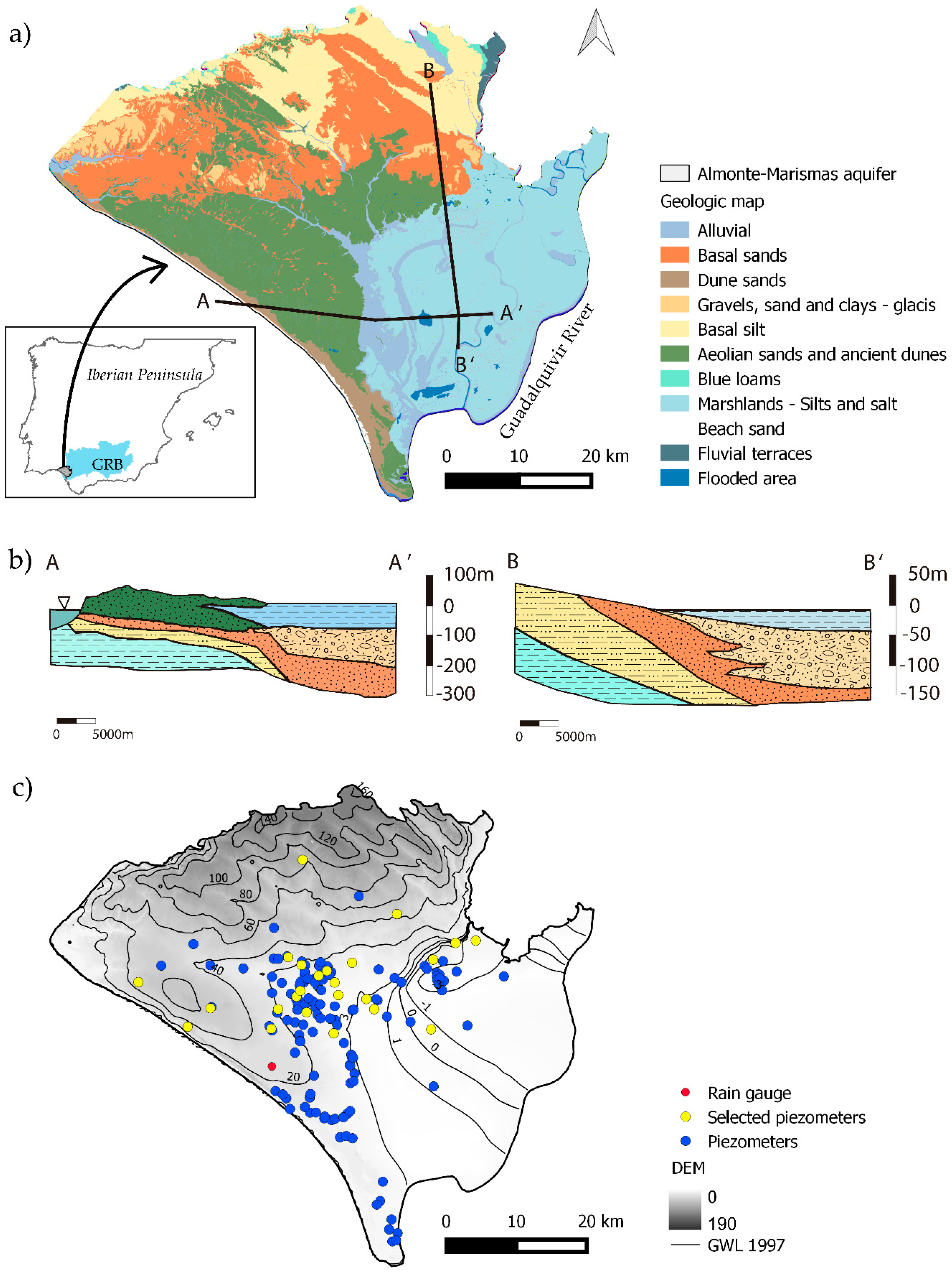
2.1. Study Site

The Almonte-Marismas aquifer, in Southwest Spain, is located at the margins of the mouth of the Guadalquivir River (Figure 1a). This aquifer hosts the Doñana marshlands, which was flooded by groundwater and surface water and declared to be RAMSAR wetlands in 1982 [24]. At the same time, Doñana water supports the socio-economic activities developed on the area, such as agriculture, industry, mining and tourism.

The topography of the region falls from approximately 150 m above sea level (masl) in the north, to less than 1 masl in the marshland area on the coast to the south. In geological terms, it is composed of a complex sedimentary system of sand and gravels with some clay lenses, basal sands, silts and aeolian sands [26,27] (Figure 1a,b). The average precipitation between 1975 and 2016 was approximately 550 mm/year and the average annual temperature was 25 °C. The maximum daily precipitation was registered at 168.2 mm in November 2001. From June to September the maximum temperature was 45 °C and the minimum temperature in winter months was 6 °C. The sub-humid Mediterranean climate with an Atlantic influence results in high seasonality [24]. The main recharge sources are rainfall, irrigation return flow and lateral inflow from the northeast. The average recharge is 200 hm³/year, primarily during spring and autumn [24]. The main groundwater flow runs from northwest to southeast, recharging mainly from the northern and southwestern areas and discharging into the Atlantic Ocean onto the marshland, rivers and streams that flow from the higher regions in the north (Figure 1c). There is no control over how much water is withdrawn for agriculture but there are estimated increases in groundwater abstraction for irrigation, from 11 hm³/year at the beginning of the 1970s to 80 hm³/year in the mid-1990s, continuing to increase up to more than 130 hm³/year, currently [28].

The Almonte-Marismas aquifer’s complex sedimentary origins, ecological richness and groundwater over-exploitation are three challenging factors for groundwater resource management decisions [27,29]. The combined effect of agricultural activities, industry and tourism have added to climate change and led to a general decrease of GWL, changing the hydrodynamics in the area [22]. As a result, several groundwater-dependent temporal ponds have disappeared [30].

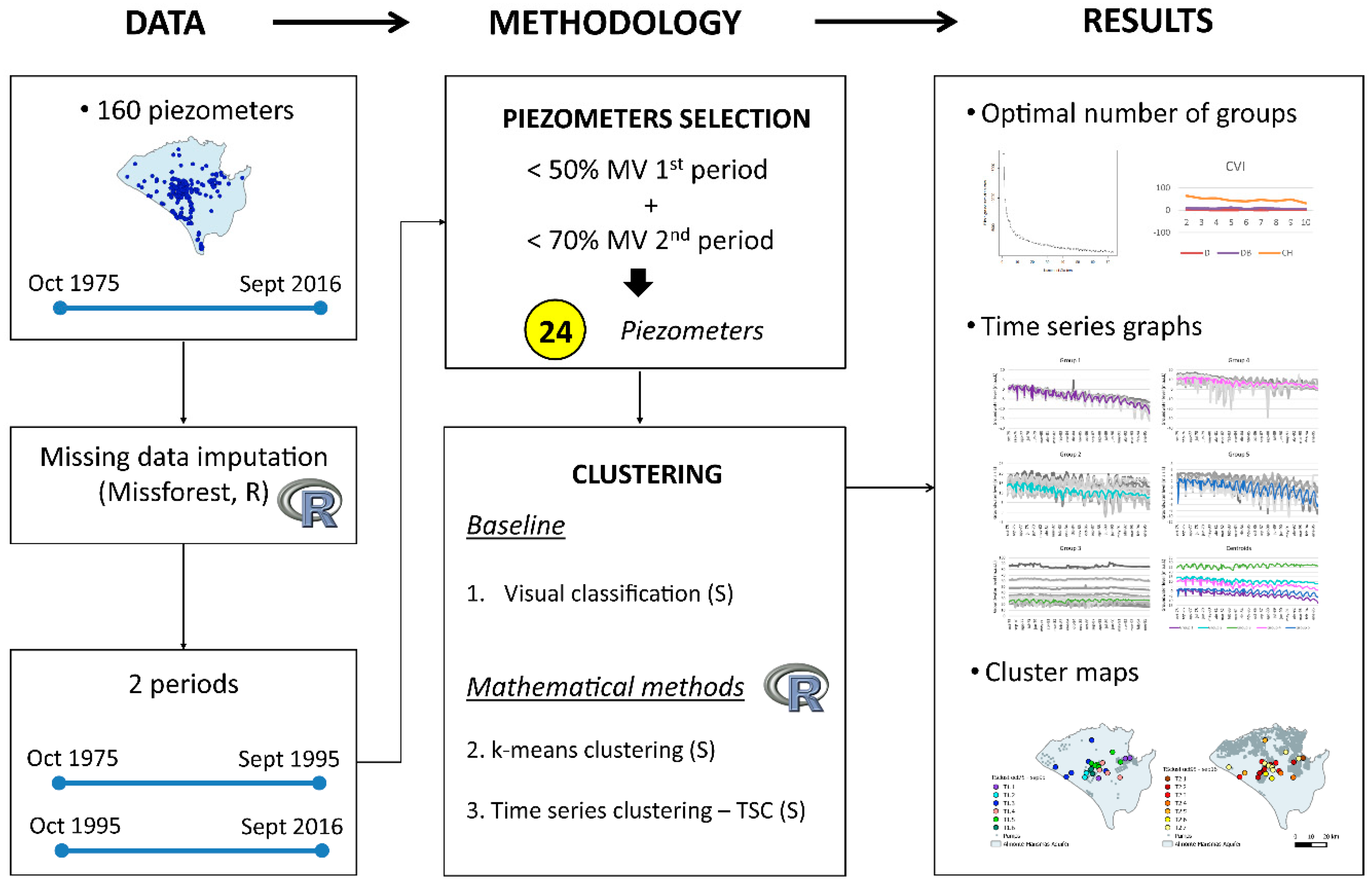
2.2. Data Collection and Pre-Treatment

Groundwater monitoring has historically been carried out in the Almonte-Marismas aquifer since 1903. Unfortunately, this GWL series does not retain continuity. Piezometers were first installed in 1970 [24], making it possible to have an entire database with 160 points (blue dots in Figure 1c) with different degrees of temporal continuity. Data from these piezometers (with less than 80% missing values (MV)), have been collected by the Spanish Geological Survey (IGME) and the CHG and have been used in the present work (yellow dots in Figure 1c). The period of time chosen, from October 1975 to September 2016, follows a hydrological year and registers the most data recorded. Agricultural activity grew considerably in the mid-1990s. Consequently, in order to analyze the evolution of the aquifer dynamics due to anthropic actions, the study period was subdivided into two sub-periods of twenty and twenty-one hydrological years: (1) October 1975–September 1995 and (2) October 1995–September 2016.

The measurements, as an absolute elevation above or under sea level, have been homogenized to a monthly time step, taking the average of all data recorded within each month. In addition, outliers and duplicates were discarded.

To study GWL responses to precipitation, rainfall data were taken from the Almonte-Acebuche rain gauge (Figure 1c), which is maintained by the AEMET (Spanish State Meteorological Agency). Cumulative deviation from the mean monthly rainfall (CDR) was calculated to represent precipitation variations in both sub-periods.

Figure 2 shows the whole approach that was followed in this study. To define a starting point (and before applying more advanced statistical techniques), visual classification of the piezometric time series was performed. This exercise is essential to developing a global understanding of the time series.

MV in the GWL time series have been infilled using all the available information (160 piezometers) and the missForest algorithm [31]. MissForest is a non-parametric, iterative imputation method, based on the random forest algorithm [32]. The advantage of missForest is that it does not make any assumptions about the distribution of data or imputation models [33]. It uses an iterative imputation scheme by training a random forest on the observed values of each variable in a first step. Then, it predicts the missing values and proceeds iteratively until the stopping criterion is met or the user-specified maximum number of iterations is reached. The algorithm continuously updates the imputed matrix variables, assessing its performance between iterations. This assessment is done by considering the difference between the previous and the new imputation results. As soon as this difference increases for the first time, the algorithm stops and keeps the last imputation matrix. The Normalized Root Mean Square Error (NRMSE; Equation (1)) has been obtained to evaluate the performance of the method:

$$\mathrm{NRMSE}=\sqrt{\frac{mean {\left(X^{true}-X^{imp}\right)}^2}{var\left(X^{true}\right)}}$$

(1)

where $X^{true}$ is the complete data matrix, $X^{imp}$ is the imputed data matrix, $mean$ and $var$ are, respectively, the short notation for the empirical mean and variance computed over the continuous missing values only. Good performance leads to a value of NRMSE close to 0 and bad performance results in a value approaching 1.

To perform a consistent GWL clustering it was decided to only use piezometers with a low percentage of MV in both study sub-periods (i.e., October 1975–September 1995 and October 1995–September 2016). The average MV percentage for the entire study period was T = 51.5%. For the first and second sub-periods the average MV percentages were P₁ = 64.1% and P₂ = 39.5%, respectively. That is the reason why a more restrictive MV threshold was applied in order to select which piezometers were used in the cluster analysis in the first sub-period, compared to the second one. The following expressions (relating P₁ and P₂ to T (Equations (2) and (3))) were used to decide which MV thresholds define what piezometers from the 160 available data points remained for the cluster analysis:

$${\mathrm{MV}}_1={\mathrm{P}}_1\left(2-{\mathrm{r}}_1\right)$$

(2)

$${ \mathrm{MV}}_2={\mathrm{P}}_2\left(1+{\mathrm{r}}_2\right)$$

(3)

where r₁ = P₁/T and r₂ = P₂/T.

Substituting P₁, P₂, r₁ and r₂ for their corresponding values in the equations yields an MV₁ threshold of 48.4% for the first sub-period and an MV₂ threshold of 69.8% for the second sub-period. Rounding up these figures, the piezometers that have less than 50% MV for the first sub-period and 70% MV for the second sub-period have been kept, resulting in 24 piezometers in total (yellow dots in Figure 1c). The general statistics for these 24 piezometers can be seen in Appendix A,

Table A1. Statistical parameters of data points.

Code	N	Mean	Med.	Max.	Min.	St. Dev	% MV
104140047	377	86.34	86.27	91.64	81.33	2.02	23.37
104180012	234	20.57	20.81	22.11	18.62	0.90	52.44
104180021	422	18.07	17.88	23.63	13.88	2.36	14.23
104210004	252	46.41	46.78	53.04	38.56	2.08	48.78
104220006	253	36.30	36.13	39.74	33.19	1.42	48.58
104230003	261	62.94	62.97	65.05	59.80	1.09	46.95
104240033	321	10.28	10.39	15.47	0.39	2.64	34.76
104240058	431	23.10	23.71	27.92	14.46	2.78	12.40
104240066	335	32.08	32.26	34.21	28.88	1.18	31.91
104240082	431	5.01	5.41	12.09	−5.48	3.81	12.40
114150046	343	8.75	8.97	11.98	6.03	1.30	30.28
114150065	404	2.37	1.94	15.50	−5.36	5.10	17.89
114160012	392	30.27	30.02	33.10	28.83	0.68	20.33
114170034	350	−7.95	−5.54	4.73	−23.19	7.59	28.86
114170040	335	−6.51	−5.36	3.89	−21.29	5.75	31.91
114180059	327	−4.35	−4.56	3.55	−12.66	3.31	33.54
114210031	235	5.45	7.87	16.44	−4.15	6.86	52.24
114210051	379	6.60	6.64	14.23	−7.06	3.87	22.97
114210076	356	2.67	2.47	6.60	−0.54	1.71	27.64
114210094	243	5.06	4.87	12.64	−2.82	3.54	50.61
114210114	338	9.65	9.50	14.20	5.98	1.98	31.30
114220007	390	1.66	1.65	5.00	−0.78	1.03	20.73
114220013	428	−1.49	−1.83	2.62	−5.52	2.50	13.01
114230024	359	−3.87	−3.88	0.86	−9.21	2.96	27.03

.

To avoid the scaling effects of GWL values while clustering, the imputed monthly piezometric series were standardized. This step was carried out before visual and k-means clustering and it is already implemented in the algorithm used to perform TSC.

2.3. K-Means Clustering

K-means clustering is one of most common methods for exploratory data analysis. This technique can identify groups in the dataset that show similar patterns or equal trends. Specifically, k-means divides up the data into pre-defined, non-overlapping groups, where every data point belongs to only one group or cluster. First of all, the random partition method randomly assigns a cluster to each observation and then the algorithm proceeds to the update step, computing the initial mean to be the centroid of the cluster’s randomly assigned points.

The standard algorithm of k-means [34] (Equation (4)), minimizes the sum of squares of the distance between data points within a cluster and the centroid of that cluster:

$$W\left(C_K\right)={\displaystyle \sum }_{X_{i }\in C_k}{\left(x_i-{\mu }_k\right)}^2$$

(4)

In the present case study, $x_i$ is the data vector with monthly measurements corresponding to piezometer $i$, $X_i$ is the set of piezometers that belongs to cluster $C_K$ and ${\mu }_k$ is the centroid, computed as the mean value of the data vector belonging to cluster $C_K$. Each data vector ($x_i$) is assigned to a cluster when its distance to the centroid, $W\left(C_K\right)$, is at a minimum.

The appropriate number of clusters is given by the point where the sedimentation graph changes the trend, drawing an “elbow” [35]. The sedimentation graph plots a clustering score as a function of the number of clusters and the elbow method is a heuristic method for interpreting and validating consistency. The score is generally a measure of the input data on the k-means objective function (e.g., sum of $W\left(C_K\right)$ across clusters). The k-means algorithm was run with the R package factoextra [36].

2.4. Time Series Clustering (TSC)

The TSC method considers time series distribution. As with the k-means method, it has a stochastic nature due to its random start. TSC was run with the R package dtwclust [15].

In order to classify all piezometers, partitional clustering [37] was selected to create partitions. The specification of the number of clusters (k) is tedious work that must be performed before starting the algorithm. The optimal k was identified by using internal clustering validity indices (CVIs). Cluster validity is a set of techniques that have been developed to find the best k without any previous class information. Based on similar works [38,39], three internal CVI indexes were used to choose k: Dunn (D), Davies–Bouldin (DB) and Calinski–Harabasz (CH). D is a ratio-type index and its cohesion is calculated by the distance to its nearest neighbor and the separation by the maximum cluster diameter [40]. DB is one of the most popular indices and it was based on the distance between centroids [41]. CH cohesion is estimated based on the distance from the points in a cluster to its centroid [42].

Depending on the distance of the disturbance and the aquifer characteristics, GWL responses can be registered with a lag of days or months from one location to another. Considering this singularity of GWL behavior, the most appropriate distance to measure GWL time series is Shape-Based Distance (SBD) [15]. SBD warps the time series and it is based on the cross-correlation with coefficient normalization ($NCCc$) and shape extraction as a prototype function (Equation (5)) [37]:

$$\mathrm{SBD}\left(x,y\right)=1-\frac{\max \left(NCCc\left(x,y\right)\right)}{{\Vert x\Vert }_2{\Vert y\Vert }_2}$$

(5)

where $\Vert \Vert {}_2$ denotes the standard L2 norm of the series and $\mathrm{SBD}\left(x,y\right)$ values range between 0 (perfect similarity) and 2 (unequal time series).

3. Results and Discussion

3.1. Imputation Piezometry and Visual Classification

Monthly imputation of the 41-year time series for the 24 piezometers with the missForest algorithm resulted in an NRMSE of 0.05, indicating a good performance of the imputation scheme. This small error can mainly be explained by the lack of uneven piezometer variations at a monthly scale, which is present in other kinds of time series (e.g., temperature), and by the high number of piezometers available for imputation.

Table 1. Number of piezometers in each obtained cluster. Sub-period 1: from October 1975 to September 1995. Sub-period 2: from October 1995 to September 2016.

Method	Sub-Period	Cluster 1	Cluster 2	Cluster 3	Cluster 4	Cluster 5	Cluster 6	Cluster 7
Visual	1	10	4	7	3	-	-	-
	2	10	5	6	3	-	-	-
k-means	1	1	2	5	1	3	12	-
	2	1	8	4	1	5	1	4
TSC	1	3	2	2	3	4	6	4
	2	1	6	4	2	2	7	2

shows how many piezometers integrate every cluster for each sub-period. Figure 3 represents the spatial distribution of the different clusters obtained. Visual classification results for both study sub-periods are shown in the first row of Figure 3a,b and in Figure 4 and Figure 5. A layer corresponding to a rough spatial distribution of the groundwater extractions in the two different sub-periods [25,43] is also included in Figure 3 (in grey). To ease the interpretation, the raw piezometric time evolution for each visual cluster is shown in Figure 4 (clusters named V1.1, V1.2, V1.3 and V1.4 for the first sub-period) and Figure 5 (clusters named V2.1, V2.2, V2.3 and V2.4 for the second sub-period). Piezometric time series are plotted in the primary Y axis with grey lines; the mean of each GWL cluster is shown in the secondary Y axis, with colored lines.

It is difficult to compare our GWL classes (Figure 3 and Figure 4) with the ones obtained from the 15 year series through visual inspection by UPC [16] and, in addition, those published in Manzano et al. [44]. These authors only showed GWL evolution at seven points within the same study area but without trying to find analogous piezometric evolution at different points.

Visual analysis found four different groups for both sub-periods. All visual cluster groups have a different spatial distribution when comparing the first and second sub-periods studied (Figure 3a,b). The main difference between the two sub-periods is that the clustering spatial distribution is more irregular in the second one. This could be attributed to an increase in the number of pumping wells (grey zones in Figure 3), in addition to climate change effects that could reduce the recharge rate [45].

At the end of the first sub-period there is a generally descending trend of GWL and a maximum average local oscillation of 5 m (Figure 4). The series that comprise groups V1.2 and V1.3 have piezometers with GWL between 0 and 80 masl, while V1.1 and V1.4 have a lower range, between −10 and 30 masl. This reflects the fact that series with visually similar GWL oscillations are located in different areas of the aquifer (Figure 3a). All of the groups exhibit time variations that may be due to extractions, as well as the recharge–discharge pattern characteristics of the hydrological cycle (e.g., compared with the CDR line). Visually, it looks like V1.1 and V1.3 are highly affected by pumping due to their cyclical oscillation over a year, ranging from 2 to 6 m. Group V1.4 seems to be located in an area exploited in the first half of the sub-period, but not in the second period. Until 1990, cluster V1.2 fluctuations followed the same temporal evolution that Custodio [4] assigned to undisturbed GWL. Furthermore, the reduced influence of anthropic actions is corroborated by the fact that piezometry has the same trend as the CDR curve (Figure 4). Among the four cluster groups, V1.4 presents the highest average level decrease of around 7 m (from 1975 to 1995). The main feature revealed by these results is that, between 1975 and 1995, anthropic impacts were already affecting the aquifer as GWL was not recuperating after the pumping cycle.

For the second sub-period, Figure 5 shows that the order of the groups from highest to lowest inter-annual oscillation is V2.2, V2.1, V2.3 and V2.4. All groups have a descending trend but at varying degrees. The V2.4 graph (Figure 5) shows the same trend as the CDR and the smallest decrease (of up to 2 m) reflects low anthropic intervention. V2.1, V2.2 and V2.3 have GWL between −10 and 40 masl and GWL in V2.4 is between 20 to 90 masl because of the altitude at the different locations. As in the first study sub-period, the wide GWL ranges are a consequence of the classification criteria (GWL behavior) and not just because of location or average values. For example, V2.4 presents a greater GWL range because two piezometers (yellow dots in Figure 3b) are located at the highest topographical area and groundwater table. V2.3 is the group with the highest drawdown in this second sub-period, up to 6 m on average. Observed drawdowns are in accordance with the piezometric descent that was estimated for the whole of the Almonte-Marismas aquifer between 1994 and 2012 (Olías-Álvarez and Rodríguez-Rodríguez [17]); this ranged from 2 to 6 m. Cluster V.2.1 shows high fluctuations of up to 4 m, attributed to pumping effects. However, time variations are similar to the ones seen in CDR, which also shows the climate response. This feature could be explained by merging climate oscillations and pumping effects seen at the locations in this cluster V2.1 (Figure 3).

Visual cluster results allow us to have an overview of the piezometer responses along each sub-period. In addition, this approach is a qualitative baseline for evaluating and comparing the results of the mathematical methods.

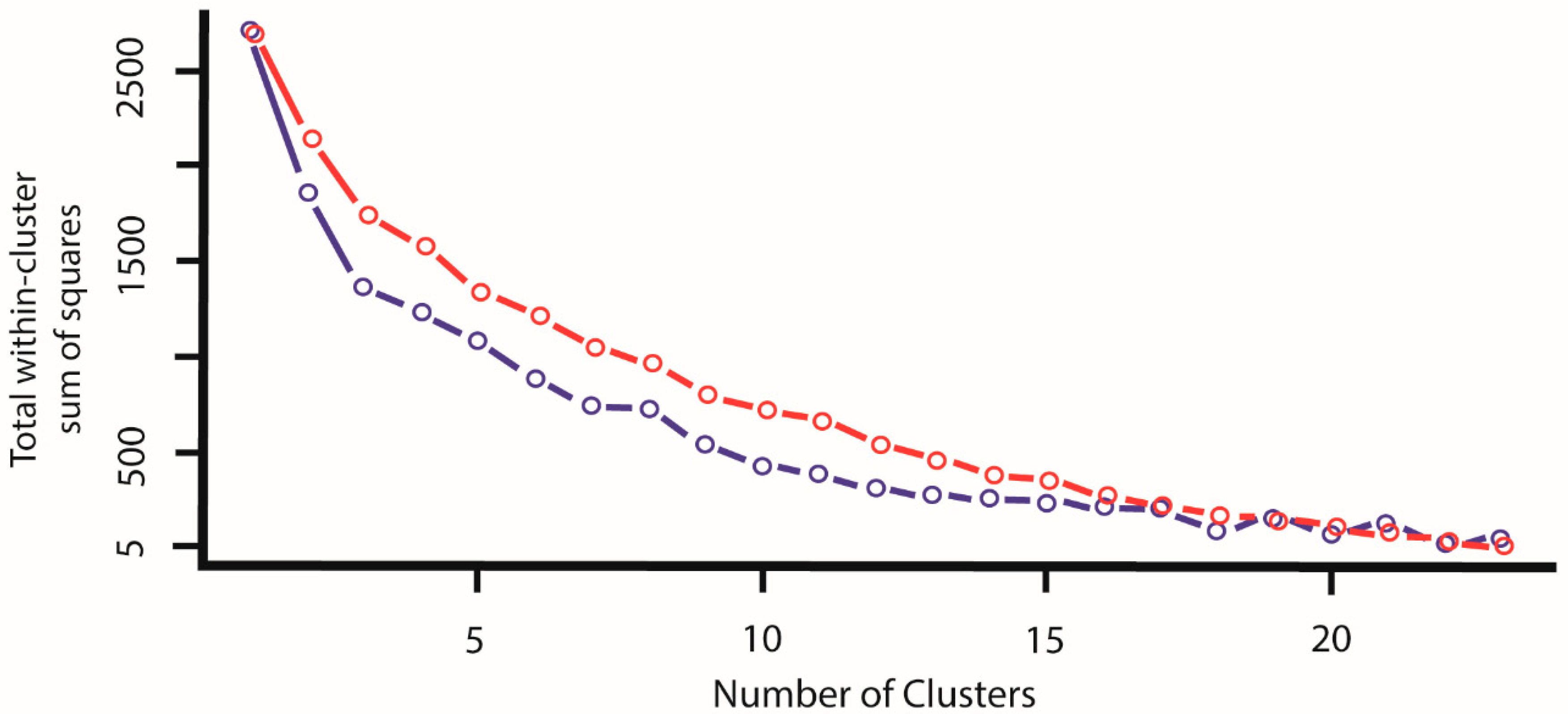
3.2. K-Means Clustering

As explained in the Section 2, when applying k-means clustering, the number of clusters k has been defined with the aid of the sedimentation graph (Figure 6). Both sedimentation curves for first (dark blue) and second (red) study sub-periods change their trend at the point which indicates the optimal number of clusters (i.e., the elbow). Both curves show smoothly decreasing trends and, given that the maximum number of clusters is 24, points around the second inflexion point in each period were tested and a final value of k chosen as a trade-off between complexity and representativeness. Consequently, k = 6 and k = 7 were taken to be the optimal number of clusters to run the k-means algorithm for the first and the second study sub-periods, respectively (Figure 6). Initially, it can be interpreted that the k-means method distinguishes more GWL variation groups that were found by visual classification. However, two and three groups are formed by just one piezometer in each sub-period. These clusters with a single piezometer correspond to singular time series variations that k-means cannot group.

As a visual classification, k-means has more spatial continuity in the cluster groups in the first sub-period than in the second period (Figure 3c,d). For both sub-periods and each k-means cluster, Figure 7 and Figure 8 plot the raw piezometric series (grey), and the average raw series (colored).

In the first sub-period, K1.3 is the group with the highest GWL range (Figure 7) due to the sparse spatial distribution of the piezometers. For example, there is one point located in the piezometric dome (Figure 1c), where important recharge rates take place. K1.3 is almost the same group as V1.2, with just one piezometer more and the same trend as the CDR. These groups of piezometers do not show fluctuations affected by direct pumping, but a decreasing trend can be seen since 1990. Groups K1.2, K1.5 and K1.6 have GWL between −10 and 30 masl and they correspond to piezometers located in the pumping areas with high anthropic changes in the natural hydrodynamics. K1.2 and K1.5 (Figure 7) have an average time series that can correspond to V1.3 (Figure 4) and K1.6 (Figure 7) corresponds to V1.1 and V1.4 (Figure 4). These groups are affected by groundwater extractions and are differently classified when using visual or k-means clustering. K1.5 and K1.6 average series show clear cycles that are attributed to the effects of groundwater extraction, as well as an important, descending trend of up to 8 m, on average (Figure 7). Spatially, they are located in an area of high agricultural development (Figure 3c). Finally, both groups K1.1 and K1.4 are composed of a single piezometer (Table 1), located in regions not affected by irrigation pumping during this first sub-period (Figure 3c).

For the second sub-period, it was observed that the GWL variations are greater than the first sub-period (Figure 8). Groups K2.1, K2.4 and K2.6 are composed of a single piezometer (Figure 8, Table 1). K2.1 is the same piezometer as K1.1. It presents a different GWL pattern than the other piezometers (with small oscillations from October 1984) and an important drawdown at the beginning of 2009 (Figure 7 and Figure 8). These abrupt variations suggest that there could be errors in the data acquisition from this piezometer. K2.4 temporal behavior indicates that aquifer exploitation started at the beginning of 2007 near this point and this could be the reason why the GWL behavior does not fit with other groups. The opposite behavior was seen in K2.6, with smooth variations during the second half of the sub-period. K2.3 does not show a clearly descending trend, with piezometers in very different areas of the aquifer (Figure 3d) and appearing as a smoothed signal of the CDR. The average series of K2.2, K2.5 and K2.7 have a decreasing tendency (Figure 8) due to the growing groundwater extractions in the nearby areas (Figure 3d). In particular, the K2.2 group presents the most pronounced drawdowns of up to 8 m, and mainly comprises piezometers located in central areas of the aquifer. It appears to correspond to an area that began to be exploited later than zone K2.5 but, as piezometry suggests, with a greater intensity reflected by a faster descent since the year 2000. The average oscillation patterns are more regular for clusters K2.5 and K2.7; this can be explained by irrigation and geological heterogeneity.

When we compare k-means results with visual classification however, some k-means groups represent a merge of hydrogeological behavior due to exploitation for irrigation of different types of crops (e.g., berries, citrus) or other uses (e.g., drinking water supply), it could be seen in the different patterns of K2.2, K2.5 and K2.7 (Figure 8). On the other hand, groups K1.3 and K2.3 have strong similitudes with the CDR graph. Similar k-means results were found by Boomfield et al. [8] with a 30-year monthly GWL series. These were in a limestone and chalk aquifer located in the UK. However, they highlight the relationship between GWL and geological characteristics for 74 points, spatially distributed across 2000 km². In the present study (and by comparing cluster spatial locations (Figure 3) with the geological distribution (Figure 1a)), it was observed that GWL are not always dependent on geology. However, cluster groups are in agreement with the findings in Boomfield et al. [8], regarding the identification of anthropogenically impacted groundwater hydrographs showing declining trends (e.g., clusters K1.6 or K2.2).

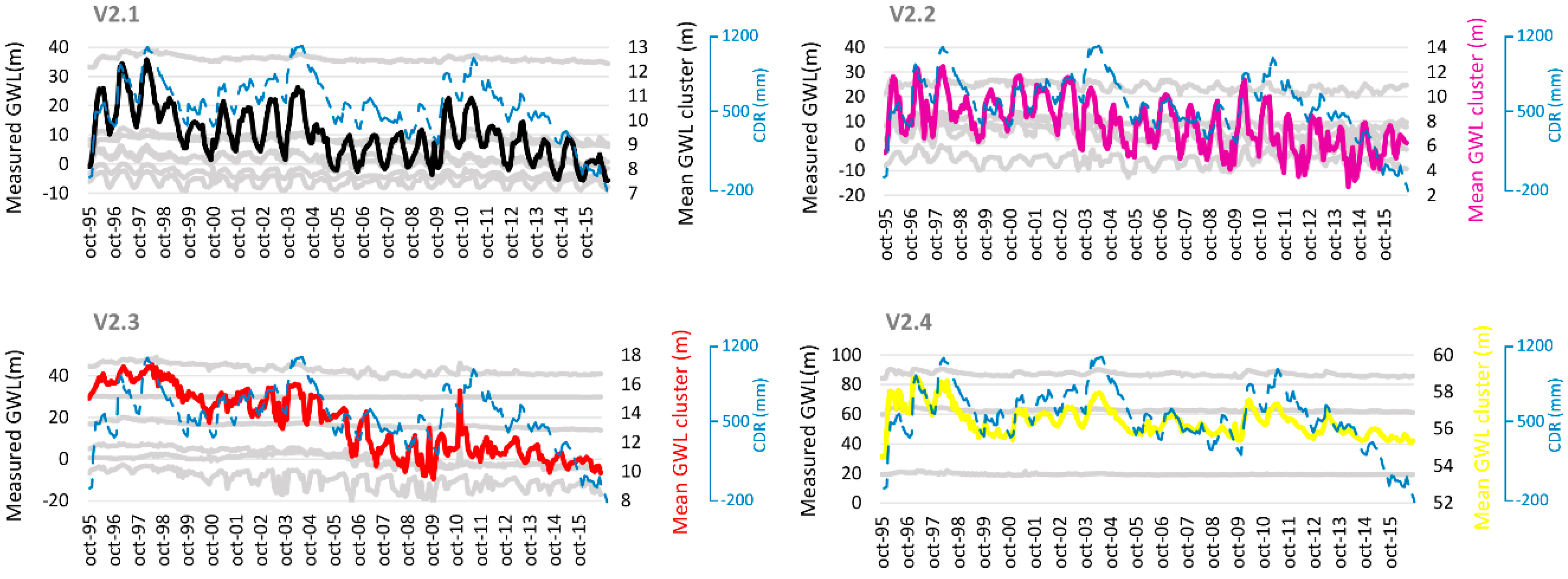
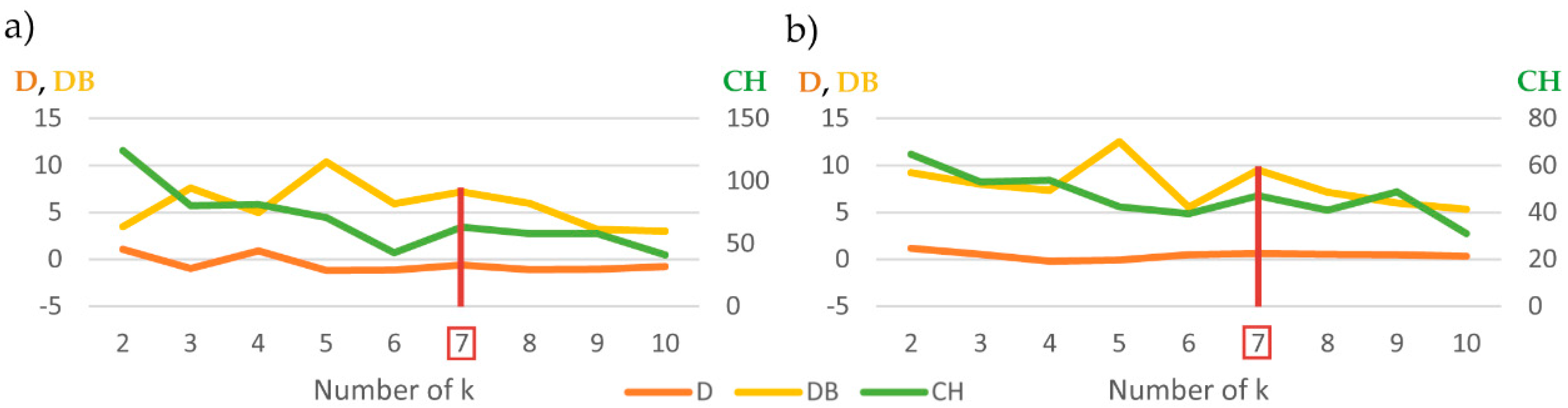
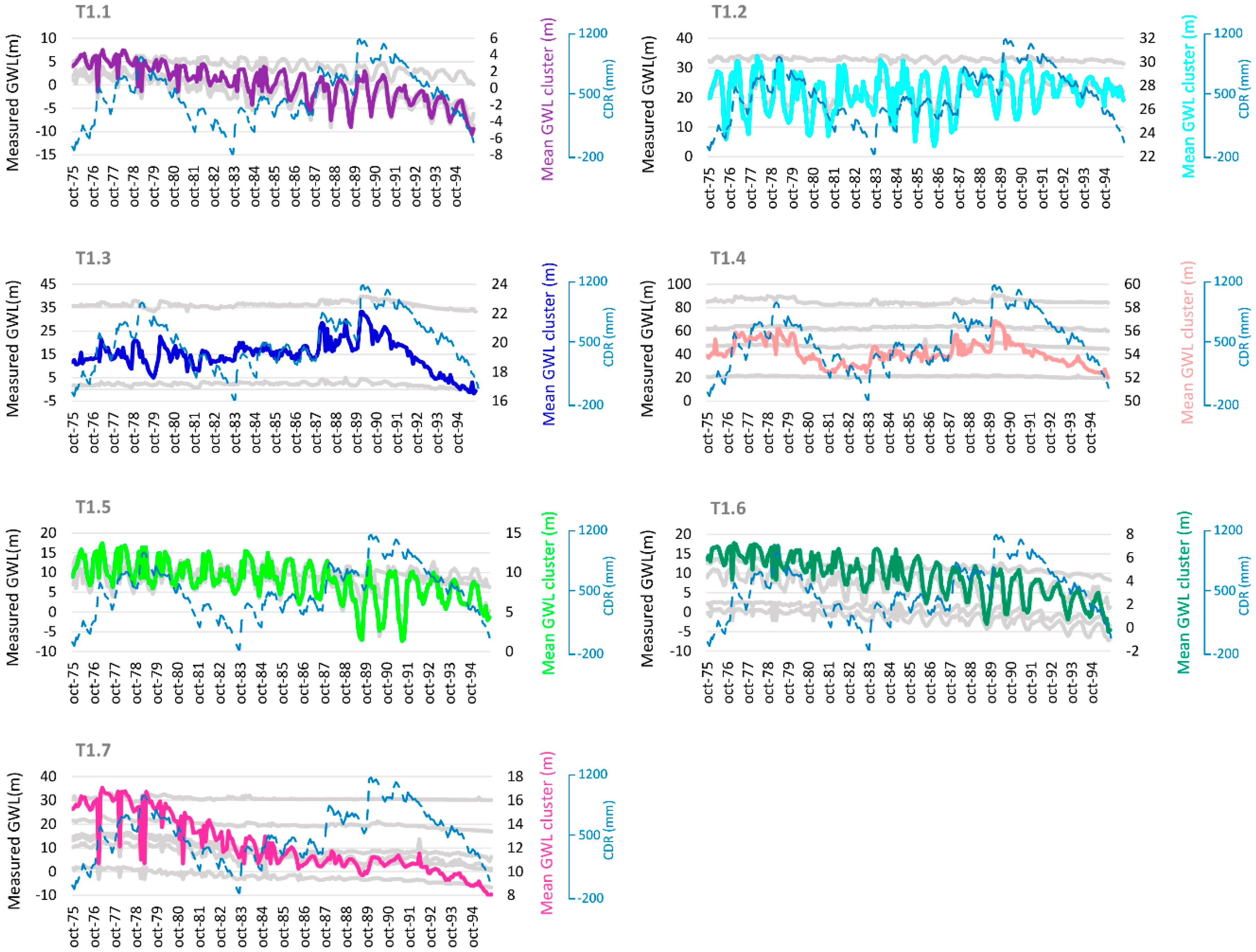
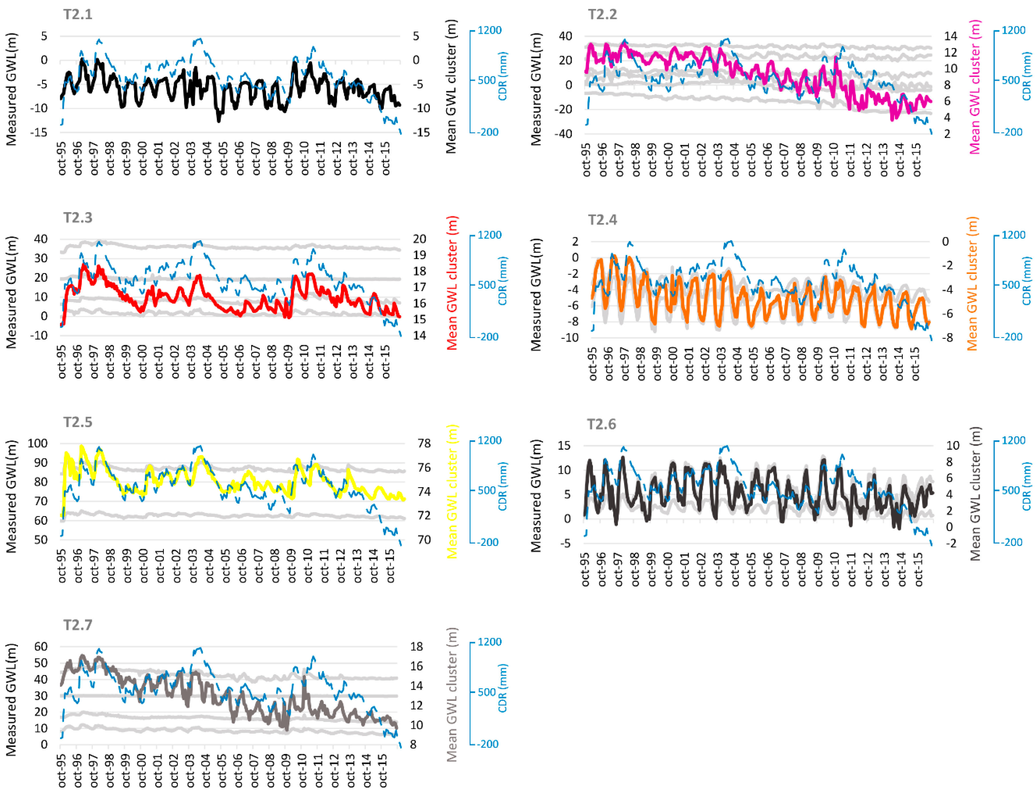
3.3. Time Series Clustering

Figure 9 shows the CVI values for a different number of clusters in both sub-periods. Following the criteria explained in Section 2, k was set to 7 in both sub-periods; D, DB and CH present an increase (marked with a red line in Figure 9). Only one of the clusters in the second sub-period had just one piezometer.

For the first sub-period, the TSC map (Figure 3e) reveals a spatial homogeneity for clusters T1.2, T1.4 and T1.5, which are located in the north and center of the aquifer. The average raw series of groups T1.3 and T1.4 (Figure 10) do not seem to have been directly influenced by agricultural pumping, due to the shape and size of their oscillations and they follow the CDR. They correspond to clusters V1.2 and K1.3, with the same decreasing trend from 1990 (Figure 4, Figure 7 and Figure 10). The T1.1 average time series is very similar to V1.1 and T1.7 to V1.4, both are affected by pumping cycles (Figure 4 and Figure 10). The rest of the groups (T1.2, T1.5 and T1.6) discriminate between different patterns that were not detected by k-means or visual classification. All of them merge annual hydrological cycles and irrigation extractions.

In the second sub-period, the spatial distribution of TSC groups is not homogeneous (Figure 3f). As in the former cluster methods, and regarding cluster series graphs (Figure 11), the general trend in the second sub-period is a GWL decrease. More specifically, T2.2, T2.4, and T2.7 have an outstanding average decrease between 2 and 10 m. Only T2.1 is composed of one piezometer (Figure 11, Table 1). T2.3 and T2.5 have similar average series and are not spatially adjacent to the irrigation areas (Figure 3f) but are closely related to the CDR. T2.2, T2.4, T2.6 and T2.7 reveal the annual oscillations associated with extractions, with average amplitudes of approximately 4 m (Figure 11). It is difficult to find correlations between these four TSC groups in the second sub-period and the visual clusters. This can be explained by the TSC’s ability to integrate different temporal hydrodynamic variations such as increasing pumping, evolution in the types of crops [46] and seasonality of GWL oscillations [47].

Comparing k-means results with TSC, the clusters reveal some similarities. For example, for the first sub-period, the location and mean graphs of pairs K1.2-T1.2 and K1.5-T1.5 are equal but K1.6-T1.7 only share the mean series shape (Figure 3, Figure 7 and Figure 10). That is the case in the second sub-period for pairs K2.2-T2.2 and K2.3-T2.3 (Figure 8 and Figure 11). For the second sub-period, the spatial distribution of the results is quite different when both methods are compared. K-means is based on the Euclidean distance between point coordinates in the feature space, thus distance is evaluated in terms of the difference between the GWL of the piezometers at the same time coordinate. Basically, k-means works by clustering together piezometers showing the least distant GWL in the complete time period vector but it does not take into account how the GWL change along the different time series. On the other hand, TSC uses the shape-based distance (SBD) that accounts for the cross-correlation between GWL series. This allows for the detecting of lagged responses in different piezometers which is, in turn, more closely related to the hydrodynamic characteristics [48]. TSC warps the series in order to fit the oscillation curves. This is confirmed by the results, for example K1.4 is composed of only one piezometer (104140047, Appendix A, Table A1). This point is far away from the other 23 points and is located in the northern part of the aquifer with a higher topographic elevation (Figure 1c). On the other hand, the same piezometer is included with another three piezometers in the T1.4 group. The average mean of T1.4 GWL series is similar to K1.4 but smoothed out. This means that there are four points with similar patterns but k-means could not detect it (Figure 7 and Figure 10). Furthermore, unlike most k-means clusters, that show relatively constant GWL trends (Figure 7 and Figure 8), several TSC clusters (T1.1, T1.6, T1.7, T2.2, T2.4 and T2.7), present clearly decreasing patterns (Figure 10 and Figure 11).

In the second sub-period, there are at least two groups with similar GWL behavior to the CDR time series. As aquifer storage is depleted because of exploitation, the rainfall dependency of the GWL response increases [49]. For the second sub-period, the mean graphs of the cluster groups (Figure 11) are more similar to CDR than the first sub-period results (Figure 10)

TSC was also successfully applied to a 0.2 km² pre-alpine Swiss shallow aquifer to investigate subsurface hydrological connectivity [10]. The authors found six groundwater response clusters over a 19 month study period. As is shown in the present work, they found that relative groundwater levels in the wells in each cluster were significantly different, in terms of amplitude and the rate of recession. Otherwise, GWL ranges in the Almonte-Marismas aquifer are quite dissimilar between piezometers belonging to the same cluster.

Rinderer et al. [10] studied a small, shallow aquifer, which is difficult to compare with the high GWL ranges of the bigger and heterogeneous Almonte-Marismas aquifer. As these authors state, grouping the groundwater dynamics into a fewer number of clusters is a gross simplification as there are obviously more types of groundwater responses. However, this clustering is a necessary step in synthetizing site-specific groundwater dynamics to general groundwater behavior. For example, TSC clusters could be used to define the over-exploitation zones in the Almonte-Marismas aquifer. Another application could be the selection of a number of key piezometers to focus the calibration process of the existing Almonte-Marismas groundwater mathematical model [25]. This will reduce the dimension of the optimization problem and, consequently, the computation time.

The most important result from TSC is the six characterized types of hydrodynamic behavior (T2.1 is a singularity) that are now present in the aquifer (Figure 11). Visually, the mean piezometric series of T2.2 is similar to that of T2.7 and the same happens with T2.4 and T2.6. The area around T2.4 is being excavated for the gravels that are under the marshlands, while gravels that are under the aeolian sands are being extracted from the area around T2.6. The different hydrogeological parameters in both cluster locations explain the differentiation in these GWL time series that cannot be seen with a qualitative comparison. In addition, the descending trends seen in T2.2 and T2.7 (from the beginning of the 2000s) are the result of uncontrolled increases in the berry fields in the northwestern part of the aquifer. This development has been denunciated by WWF on several occasions [21]. On the other hand, clusters T2.3 and T2.5 are less anthropically influenced but are more affected by recharge fluctuations.

On a global scale, GWL time series clustering can contribute to the identification and separation of spatiotemporal processes associated with both climate and human disturbances. This separation is often tackled through complex transfer function-noise models [50,51]. Similar aquifer exploitation regimes in different countries or regions could then be clustered together and provide the basis to build time series classification models based on labeled time series resulting from the clustering analysis. In turn, this would support the development of global actions for sustainable groundwater management.

4. Conclusions

The main goals of this work were to study the historical piezometry of the Almonte-Marismas Aquifer, to improve the knowledge about hydrodynamics and to prove that anthropic activities have changed GWL trends in the system. It was possible to reach these aims by analyzing the historic piezometric database (for a period of over 41 hydrological years), applying two robust clustering methods, comparing the results and highlighting the advantages and disadvantages of both. Temporal changes in the variables that affect GWL (recharge, water exploitation, climate change, surface/groundwater interactions) could help to explain the visual, k-means and TSC results. The study period was divided in two in order to search for important piezometric changes due to the growing demand of irrigation fields. The differences observed between the GWL clusters for the first and the second sub-periods reflect the influence of the socioeconomic and anthropic development on the natural regime. The relationship between CDR and GWL decreases with anthropic exploitation, making aquifer storage more vulnerable to the effects of climate change but the response of GWL to rainfall events becomes quicker when the aquifer is over-exploited. The natural system exhibits complex hydrological behavior, highlighting the need to adapt water policy and management to every single case.

Visual clustering offers a first approach to characterizing the behavior of the hydrographs, considering expert judgement and providing a basis for the validation of mathematical methods. However, in the second study sub-period, it was observed that the combination of extractions (in terms of quantity and time of year) produces a merging of responses in which there is no clear spatial correspondence. More specifically, k-means methodology allows the distinguishing of singular GWL oscillations, assigning piezometers to classes with only one GWL point. This permits the identification of errors in data measurements or temporal changes in the external factors that does not occur in other areas of the aquifer. In areas not affected by groundwater extractions, k-means classification gives similar results to visual classification.

Our findings confirm that TSC offers better results for studying time series distribution because the members of the same group reproduce the same pattern. K-means considers time (average monthly GWL as attributes for each piezometer) but not the correlation structure of the time series. This is an important limitation to detecting changes in temporal patterns in different groups. TSC considers the time series distribution and the results show consistent distribution of GWL responses. Further studies will facilitate the introduction of cluster results, in order to optimize and reduce the amount of input data for mathematical groundwater flow models, contributing to the speeding up and simplifying of the modelling process. Also, the obtained results could offer a way to zone the effects of uncontrolled exploitation wells by estimating the extent of the effects of water extractions. The new characterization of the Doñana piezometry, based on a long GWL series and TSC objective criteria, proves the important impact that uncontrolled extraction has had over a period of decades.

References

1. Álvarez-Cobelas, M.; Cirujano, S.; Sánchez-Carrillo, S. Hydrological and botanical man-made changes in the Spanish wetland of Las Tablas de Daimiel. Biol. Conserv. 2001, 97, 89–98. [Google Scholar] [CrossRef]
2. Castellazzi, P.; Martel, R.; Rivera, A.; Huang, J.; Pavlic, G.; Calderhead, A.I.; Chaussard, E.; Garfias, J.; Salas, J.; Goran, P. Groundwater depletion in Central Mexico: Use of GRACE and InSAR to support water resources management. Water Resour. Res. 2016, 52, 5985–6003. [Google Scholar] [CrossRef]
3. Lubis, R.F. Urban hydrogeology in Indonesia. IOP Conf. Ser. Earth Environ. Sci. 2018, 118, 012022. [Google Scholar] [CrossRef]
4. Custodio, E. Aquifer overexploitation: What does it mean? Hydrogeol. J. 2002, 10, 254–277. [Google Scholar] [CrossRef]
5. Díaz-Paniagua, C.; Zamudio, R.F.; Florencio, M.; Murillo, P.G.; Rodríguez, C.G.; Portheault, A.; Martín, L.S.; Siljestrom, P. Temporay ponds from Doñana National Park: A system of natural habitats for the preservation of aquatic flora and fauna. Limnetica 2010, 29, 41–58. [Google Scholar]
6. Green, A.J.; Alcorlo, P.; Peeters, E.T.; Morris, E.; Espinar, J.L.; Bravo-Utrera, M.A.; Bustamante, J.; Díaz-Delgado, R.; Koelmans, A.; Mateo, R.; et al. Creating a safe operating space for wetlands in a changing climate. Front. Ecol. Environ. 2017, 15, 99–107. [Google Scholar] [CrossRef] [Green Version]
7. Irawan, D.E.; Puradimaja, D.J.; Notosiswoyo, S.; Soemintadiredja, P. Hydrogeochemistry of volcanic hydrogeology based on cluster analysis of Mount Ciremai, West Java, Indonesia. J. Hydrol. 2009, 376, 221–234. [Google Scholar] [CrossRef]
8. Bloomfield, J.; Marchant, B.; Bricker, S.H.; Morgan, R.B. Regional analysis of groundwater droughts using hydrograph classification. Hydrol. Earth Syst. Sci. 2015, 19, 4327–4344. [Google Scholar] [CrossRef] [Green Version]
9. Nakagawa, K.; Yu, Z.-Q.; Berndtsson, R.; Kagabu, M. Analysis of earthquake-induced groundwater level change using self-organizing maps. Environ. Earth Sci. 2019, 78. [Google Scholar] [CrossRef]
10. Rinderer, M.; Van Meerveld, I.; McGlynn, B.L. From Points to Patterns: Using Groundwater Time Series Clustering to Investigate Subsurface Hydrological Connectivity and Runoff Source Area Dynamics. Water Resour. Res. 2019, 55, 5784–5806. [Google Scholar] [CrossRef]
11. Yuan, R.; Wang, M.; Wang, S.; Song, X. Water transfer imposes hydrochemical impacts on groundwater by altering the interaction of groundwater and surface water. J. Hydrol. 2020, 583, 124617. [Google Scholar] [CrossRef]
12. Asgharinia, S.; Petroselli, A. A comparison of statistical methods for evaluating missing data of monitoring wells in the Kazeroun Plain, Fars Province, Iran. Groundw. Sustain. Dev. 2020, 10, 100294. [Google Scholar] [CrossRef]
13. Celestino, A.M.; Cruz, D.M.; Otazo-Sánchez, E.; Reyes, F.G.; Soto, D.V. Groundwater Quality Assessment: An Improved Approach to K-Means Clustering, Principal Component Analysis and Spatial Analysis: A Case Study. Water 2018, 10, 437. [Google Scholar] [CrossRef] [Green Version]
14. Bottou, L.; Bengio, Y. Convergence properties of the k-mean algorithms. In Neural Information Processing Systems 7 (NIPS 1994); MIT Press: Denver, CO, USA, 1995; pp. 585–592. [Google Scholar]
15. Sardá-Espinosa, A. Time-Series Clustering in R Using the Dtwclust Package. Available online: https://journal.r-project.org/archive/2019/RJ-2019-023/RJ-2019-023.pdf (accessed on 2 November 2019).
16. UPC. Regional Groundwater Flow in the Almonte-Marismas Aquifer; Groundwater Hydrology Group of the Technical University of Catalonia and Geological Institute of Spain: Madrid, Spain, 1999; p. 114. [Google Scholar]
17. Olías Álvarez, M.; Rodríguez Rodríguez, M. Evolución de los niveles en la red de control piezométrica del acuífero Almonte-Marismas (periodo 1994–2012). In Proceedings of the X Simposio de Hidrogeología, Hidrogeología y Recursos Hidráulicos, Granada, Spain, 16–18 October 2013; Volume 30, pp. 1.121–1.130. [Google Scholar]
18. CHG. Informe De Seguimiento Del Plan Hidrológico De La Demarcación Hidrográfica Del Guadalquivir; Ciclo de Planificación 2015–2021; Ministerio de Transición Ecológica: Madrid, Spain, 2019.
19. Nguyen, T.T.; Kawamura, A.; Tong, T.N.; Nakagawa, N.; Amaguchi, H.; Gilbuena, R. Clustering spatio–seasonal hydrogeochemical data using self-organizing maps for groundwater quality assessment in the Red River Delta, Vietnam. J. Hydrol. 2015, 522, 661–673. [Google Scholar] [CrossRef]
20. Guardiola-Albert, C.; Jackson, C.R. Potential Impacts of Climate Change on Groundwater Supplies to the Doñana Wetland, Spain. Wetlands 2011, 31, 907–920. [Google Scholar] [CrossRef] [Green Version]
21. WWF. Salvemos Doñana. Del Peligro a la Prosperidad. 2016. Available online: http://awsassets.wwf.es/downloads/wwf_informe_salvemos_donana__2016.pdf?_ga=2.266321487.1975888914.1579078039-1333755382.1573218666 (accessed on 15 January 2020).
22. Erostate, M.; Huneau, F.; Garel, E.; Ghiotti, S.; Vystavna, Y.; Garrido, M.; Pasqualini, V. Groundwater dependent ecosystems in coastal Mediterranean regions: Characterization, challenges and management for their protection. Water Res. 2020, 172, 115461. [Google Scholar] [CrossRef]
23. MacQueen, J. Some Methods for Classification and Analysis of Multivariate Observations. In Proceedings of the Fifth Berkeley Symposium on Mathematical Statistics and Probability; University of California Press: Berkeley, CA, USA, 1967; Volume 1, pp. 281–297. Available online: http://projecteuclid.org:443/euclid.bsmsp/1200512992 (accessed on 10 January 2020).
24. Custodio, E.; Manzano, M.; Montes, C. Las Aguas Subterráneas En Doñana; Aspectos Ecológicos y Sociales; Junta de Andalucía: Sevilla, Spain, 2009; p. 244. ISBN 978-84-92807-19-2.
25. Guardiola-Albert, C.; García-Bravo, N.; Mediavilla, C.; Martín Machuca, M. Gestión de los recursos hídricos subterráneos en el entorno de Doñana con el apoyo del modelo matemático del acuífero Almonte-Marismas. Bol. Geol. y Min. 2009, 120, 361–376, ISSN 0366-0176. [Google Scholar]
26. Salvany, J.M.; Custodio, E. Características litoestratigráficas de los depósitos pliocuaternarios del bajo Guadalquivir en el área de Doñana: Implicaciones hidrogeológicas. Rev. de la Soc. Geol. de Esp. 1995, 8, 21–31. [Google Scholar]
27. Salvany, J.M.; Larrasoaña, J.C.; Mediavilla, C.; Rebollo, A. Chronology and tectono-sedimentary evolution of the Upper Pliocene to Quaternary deposits of the lower Guadalquivir foreland basin, SW Spain. Sediment. Geol. 2011, 241, 22–39. [Google Scholar] [CrossRef] [Green Version]
28. CHG. Propuesta para la Declaración de la Masa de Aagua Subterránea de la Rocina en Riesgo de no Aalcanzar uun Buen Estado Cuantitativo y Guímico; Ministerio de Transición Ecológica: Madrid, Spain, 2019.
29. Carnicer i Cols, J. Species richness, interaction networks, and diversification in bird communities: A synthetic ecological and evolutionary perspective. Bellaterra: Universitat Autònoma de Barcelona, 2008. ISBN 9788469139042. Tesis doctoral - Universitat Autònoma de Barcelona, Facultat de Ciències, Departament de Biologia Animal, Biologia Vegetal i Ecologia. 2007. Available online: https://ddd.uab.cat/record/36713 (accessed on 10 December 2019).
30. Diaz-Paniagua, C.; Fernández-Zamudio, R.; Florencio, M.; García-Murillo, P.; Gómez-Rodríguez, J.M.; Siljeström, P.; Serrano, L. The temporary ponds of Doñana: Conservation value and present tretas. Eur. Pond Conserv. Netw. Newsl. 2008, 1, 5–685. [Google Scholar]
31. Stekhoven, D.J.; Bühlmann, P. Miss-Forest? Non parametric missing value imputation for mixed-type data. Bioinformatics 2011, 28, 112–118. [Google Scholar] [CrossRef] [PubMed] [Green Version]
32. Breiman, L. Random Forests. Mach. Learn. 2001, 45, 5–32. [Google Scholar] [CrossRef] [Green Version]
33. Aguilera, H.; Guardiola-Albert, C.; Naranjo-Fernández, N.; Kohfahl, C. Towards flexible groundwater-level prediction for adaptive water management: Using Facebook’s Prophet forecasting approach. Hydrol. Sci. J. 2019, 64, 1504–1518. [Google Scholar] [CrossRef]
34. Hartigan, J.A.; Wong, M.A. Algorithm AS 136: A K-Means Clustering Algorithm. Appl. Stat. 1979, 28, 100. [Google Scholar] [CrossRef]
35. Ketchen, D.J.; Shook, C.L. The application of cluster analysis in Strategic Management Research: An analysis and critique. Strateg. Manag. J. 1996, 17, 441–458. [Google Scholar] [CrossRef]
36. Kassambara, A.; Mundt, F. Factoextra: Extract and Visualize the Results of Multivariate Data Analyses. 2017. Available online: http://www.sthda.com/english/rpkgs/factoextra (accessed on 12 December 2019).
37. Paparrizos, J.; Gravano, L. k-Shape: Efficient and Accurate Clustering of Time Series. In Proceedings of the 2015 ACM SIGMOD International Conference on Management of Data—SIGMOD ’15, Portland, OR, USA, 14–19 June 2020; Association for Computing Machinery (ACM): New York, NY, USA, 2015; pp. 1855–1870, ISBN 978-1-4503-2758-9. [Google Scholar] [CrossRef]
38. Maulik, U.; Bandyopadhyay, S. Performance evaluation of some clustering algorithms and validity indices. IEEE Trans. Pattern Anal. Mach. Intell. 2002, 24, 1650–1654. [Google Scholar] [CrossRef] [Green Version]
39. Kryszczuk, K.; Hurley, P. Estimation of the Number of Clusters Using Multiple Clustering Validity Indices. In Multiple Cassifier Systems; El Gayar, N., Kittler, J., Roli, F., Eds.; MSC 2010. Lecture Notes in Computer Science; Springer: Berlin/Heidelberg, Germany, 2010; Volume 5997, pp. 114–123. [Google Scholar]
40. Dunn, J.C. A fuzzy relative of the ISODARA process and its use in detecting compact well-separated clusters. J. Cybern. 1973, 3, 32–57. [Google Scholar] [CrossRef]
41. Davies, D.L.; Bouldin, D.W. A Cluster Separation Measure. IEEE Trans. Pattern Anal. Mach. Intell. 1979, 1, 224–227. [Google Scholar] [CrossRef]
42. Calinski, T.; Harabasz, J. A dendrite method for cluster analysis. Commun. Stat. 1974, 3, 1–27. [Google Scholar]
43. Manzano, M.; Custodio, E.; Montes, C.; Mediavilla, C. Groundwater Quality and Quantity Assessment through a Dedicated Monitoring Network: The Doñana Aquifer Experience (SW Spain). Groundwater Monitoring; John Wiley & Sons: Hoboken, NJ, USA, 2009; pp. 273–287. [Google Scholar]
44. Manzano, M.; Borja, F.; Montes, C. Metodología de tipificación hidrología de los humedales españoles con vistas a su valoración funcional y a su gestión. Aplicación a los humedales de Doñana. Bol. Geol. Min. 2002, 113, 313–330, ISSN 0366-0176. [Google Scholar]
45. Naranjo-Fernández, N.; Guardiola-Albert, C.; Aguilera, H.; Serrano-Hidalgo, C.; Rodríguez-Rodríguez, M.; Fernández-Ayuso, A.; Ruiz-Bermudo, F.; Montero-González, E. Relevance of spatio-temporal rainfall variability regarding groundwater management challenges under global change: Case study in Doñana (SW Spain). Stoch. Environ. Res. Risk Assess. 2020. [Google Scholar] [CrossRef]
46. Fundación Doñana 21. Bases estratégicas para una agricultura sostenible en Doñana. Área de agricultura. 2003. Available online: http://donana.es/source/BASES%20ESTRATEGICAS%20PARA%20UNA%20AGRICULTURA%20SOSTENIBLE%20EN%20DO%C3%91ANA.pdf (accessed on 20 February 2020).
47. Fernández-Ayuso, A.; Aguilera, H.; Guardiola-Albert, C.; Rodríguez-Rodríguez, M.; Heredia, J.; Naranjo-Fernández, N. Unraveling the Hydrological Behavior of a Coastal Pond in Doñana National Park (Southwest Spain). Groundwater 2019, 57, 895–906. [Google Scholar] [CrossRef]
48. Guijo-Rubio, D.; Rosal, A.M.D.; Gutiérrez, P.A.; Troncoso, A.; Hervas-Martínez, C. Time series clustering based on the characterisation of segment typologies. arXiv 2018, arXiv:1810.11624v1. [Google Scholar]
49. Lorenzo-Lacruz, J.; Garcia, C.; Morán-Tejeda, E. Groundwater level responses to precipitation variability in Mediterranean insular aquifers. J. Hydrol. 2017, 552, 516–531. [Google Scholar] [CrossRef]
50. Shapoori, V.; Peterson, T.J.; Western, A.; Costelloe, J. Top-down groundwater hydrograph time-series modeling for climate-pumping decomposition. Hydrogeol. J. 2015, 23, 819–836. [Google Scholar] [CrossRef]
51. Van Dijk, W.M.; Densmore, A.L.; Jackson, C.R.; Mackay, J.D.; Joshi, S.K.; Sinha, R.; Shekhar, S.; Gupta, S. Spatial variation of groundwater response to multiple drivers in a depleting alluvial aquifer system, northwestern India. Prog. Phys. Geogr. Earth Environ. 2019, 44, 94–119. [Google Scholar] [CrossRef] [Green Version]
Figure 1. (a) Location and geological map; (b) Cross sections of Almonte-Marismas aquifer (Guadalquivir River Basin, GRB); and (c) Piezometers and Almonte-Acebuche rain gauge locations and piezometric surface at the end of 1997, taken from Guardiola-Albert et al. [25]. DEM: Digital Elevation Model.
Water 12 01063 g001
Figure 2. Flowchart of the methodological approach used in the current study. S: standardization as pre-treatment.
Water 12 01063 g002
Figure 3. Spatial distribution of piezometer groups for the three clustering methods applied. An approximate distribution of the pumping wells [25,43] is shown in grey. (a) Visual clustering for first sub-period (October 1975 to September 1995); (b) Visual clustering for second sub-period (October 1995 to September 2016); (c) k-means clustering for first sub-period; (d) k-means clustering for second sub-period; (e) Time series clustering (TSC) for first sub-period; (f) TSC for second sub-period.
Water 12 01063 g003
Figure 4. Groundwater levels (GWL) series (grey lines), mean of the GWL cluster series (colored lines) from October 1975 to September 1995 by visual clustering and cumulative deviation from the mean monthly rainfall (CDR).
Water 12 01063 g004
Figure 5. GWL series (grey lines), mean of the GWL cluster series (colored lines) from October 1995 to September 2016 by visual clustering and cumulative deviation from the mean monthly rainfall (CDR).
Water 12 01063 g005
Figure 6. K-means sedimentation graphs of cluster sub-periods. Blue dots represent the first sub-period (from October 1975 to September 1995) and red dots the second sub-period (from October 1995 to September 2016).
Water 12 01063 g006
Figure 7. GWL series (grey lines), mean of the GWL cluster series (colored line) from October 1975 to September 1995 (first sub-period), classified by k-means clustering and cumulative deviation from the mean monthly rainfall (CDR).
Water 12 01063 g007
Figure 8. GWL series (grey lines), mean of the GWL cluster series (colored line) from October 1995 to September 2016 (second sub-period), classified by k-means clustering and cumulative deviation from the mean monthly rainfall (CDR).
Water 12 01063 g008
Figure 9. Cluster Validity Indices (CVI): Dunn (D), Davies–Bouldin (DB) and Calinski–Harabasz (CH). X axes represent the number of clusters (k) and Y axes are the sum-of-squares. D and DB are represented in the primary Y axis and CH in the secondary Y axis. (a) CVI for first sub-period (October 1975 to September 1995). (b) CVI for second sub-period (October 1995 to September 2016).
Water 12 01063 g009
Figure 10. GWL series (grey lines), mean of the GWL cluster series (colored line) from October 1975 to September 1995 (first sub-period), classified by TSC, and cumulative deviation from the mean monthly rainfall (CDR).
Water 12 01063 g010
Figure 11. GWL series (grey lines), mean of the GWL cluster series (colored line) from October 1995 to September 2016 (second sub-period), classified by TSC, and cumulative deviation from the mean monthly Rainfall (CDR).
Water 12 01063 g011