Analyzing the Effectiveness of a Multi-Purpose Dam Using a System Dynamics Model

Department of Civil Engineering, Kyung Hee University, 1732 Deogyeong-daero, Giheung-gu, Yongin-si, Gyeonggi-do 17104, Korea
*
Author to whom correspondence should be addressed.
Water 2020, 12(4), 1062; https://doi.org/10.3390/w12041062
Submission received: 12 February 2020
/
Revised: 25 March 2020
/
Accepted: 7 April 2020
/
Published: 8 April 2020
(This article belongs to the Special Issue Application of the Systems Approach to the Management of Complex Water Systems)
Abstract
:The increasing frequency of extreme droughts and flash floods in recent years due to climate change has increased the interest in sustainable water use and efficient water resource management. Because the water resource sector is closely related to human activities and affected by interactions between the humanities and social sciences, there is a need for interdisciplinary research that can consider various elements, such as society and the economy. This study elucidates relationships within the social and hydrological systems and quantitatively analyzes the effects of a multi-purpose dam on the target society using a system dynamics model. A causal loop was used to identify causal relationships between the social and hydrological components of the target area, and a simulation model was constructed using the system dynamics technique. Additionally, climate change and socio-economic scenarios were applied to analyze the future effects of the multi-purpose dam on population change, the regional economy, water use, and flood damage prevention in the target area. The model proved reliable in predicting socio-economic changes in the target area and can be used to make decisions about efficient water resource management and water-resource-related facility planning.
1. Introduction
1.1. System Dynamics Approach for Water Management under Changing Environment
Water resource development studies originally focused on understanding natural phenomena and on securing water resources. However, economic and social developments have necessitated studies that consider not only engineering elements, but also their relationships with various human and social elements, such as the economy, environment, and ecosystems. In recent years, interest in securing and using sustainable water resources has increased due to the influence of climate change. The water-resource sector is closely related to human activities, and they interact in more complex forms because of diverse and complex changes in the humanities and social sciences. Therefore, the interdisciplinary study to quantify the mutual effects of water resources and socio-economic factors is potentially useful for establishing water resource policies and planning for large-scale water resource facilities.
During the past five decades, a systems approach has been applied in many practical and scientific fields, including management, ecology, economics, education, engineering, public health, and sociology [1]. Among the systems analysis techniques, the system dynamics (SD), feedback-based and object-oriented simulation approach, can define the complex relationships in water resources systems and understand the dynamic correlation between socio-economic and hydrological systems according to causality between the system components [2]. The SD scheme is popular because of its advantages to handle the complex interactions among system components [3]. It studies the dynamic, evolving, cause-effect interrelations, and information feedbacks that direct interactions in a system over time [4,5]. Using the SD approach, we can understand more accurately and fundamentally the problems surrounding the water resources environment in an interdisciplinary modeling framework [6].
1.2. Literature Review of Systems Approaches for Water Resources Management
A hydro-system contains disparate but interactive components, which function as a unit and should be handled as a whole [7]. The SD has been applied in the hydro-system modeling and water resource management for more than 20 years [8]. Some representative SD application literature in the water field are summarized as follows.
Ahmad and Simonovic [6] developed a system dynamics model for the simulation of reservoir operation for flood management. The reservoir operation rules were suggested for high flow/flood years for mitigation of flooding by changing the reservoir storage allocation, reservoir levels and outflows in the Shellmouth reservoir on the Assiniboine River in Canada. The developed model was beneficial to predict future system behavior and provide a decision for secured flood management.
Li and Simonovic [9] developed a model to simulate flood patterns by snowmelt under temperature change in the spring season. The model is composed of five tanks representing snow, interception, surface, subsurface and groundwater storage and capture a vertical water balance. They studied hydrological processes in North American prairie watersheds where floods are significantly contributed to by snowmelt. They found that snowpack accumulation and snowmelt are major importance on flood generation and the temperature is a critical factor to determine the snowmelt rate and the physical state of the soil.
Simonovic [10] developed a global water model (named, World Water Model), and conducted a macro-scale assessment of global water resources availability. The study showed the relationship between water resources and future industrial growth and revealed that water pollution is the most important water problem in the future.
Xu et al. [2] constructed a simulation model to evaluate the sustainability of the water resources system in the Yellow River basin. The model captured the dynamic characteristics of the main components affecting water demand and supply. Scenario analyses were conducted by predicting future water demand and supply conditions and evaluated future water sustainability in different sub-regions.
Stave [11] carried out a study to encourage the public to understand the value of water conservation in Las Vegas, Nevada. The study described the process of building a strategic-level system dynamics model for water management of the study area.
Simonovic and Rajasekaram [12] developed an Integrated Water Resources Management (IWRM) model, in which the dynamic interactions between the quantitative features of available water resources and the water use affected by socio-economic levels of development, population and physiological features were simulated. The study developed 12 scenarios to investigate policy options in wastewater treatment, economic and population growth, freshwater export, energy production and trade.
Neto et al. [13] developed a system dynamics model to analyze the complicated interrelationships among the agents affecting the Sepetibza Bay environment. The model simulated various hypotheses of economic growth and population increase on the watershed. The study explained how environmental problems should be managed when the industry and population are expected to grow rapidly. Furthermore, a model simulation through system dynamics can provide important information to the policy decision-makers and the public related to water resources management.
Madani and Mariño. [14] conducted an integrated study and suggested a model based on a causal loop to manage the complicated water system. The study showed that diverse options of demand management and population control can be effective in addressing the water crisis, increasing water storage capacity and controlling of groundwater withdrawal.
Khan et al. [15] developed a conceptual water balance model to simulate the hydrologic processes including percolation, surface runoff, actual evapotranspiration, and capillary rise. Using the model, the dynamic interactions between surface and groundwater in an irrigation area was simulated. The model further applied to simulate responses of different irrigation management scenarios and reduce the cost of groundwater abstraction in lowland areas.
Davies and Simonovic [16] developed an integrated assessment model, ANEMI, which represents nonlinear feedbacks between water resources, socio-economic, and environmental systems. The model includes eight sectors, such as climate, carbon cycle, economy, land use, agriculture, population, natural hydrological cycle, water use and quality.
Gaupp et al. [17] examined how storage capacity can improve water security in large river basins using a water balance model. The model can simulate runoff, water use from surface and aquifer, evaporation and trans-boundary discharges in BCUs (basin country unit) scale. The study showed the balance between water for human use and water for the environment and helped to acknowledge the limitations of over-reliance on water storage.
Di Baldassarre et al. [18] analyzed the system dynamics between supply–demand cycles and reservoir effects using a causal loop diagram and demonstrated the case studies in Athens, Las Vegas and Melbourne. The reservoir effect showed that the construction of reservoirs can supply abundant water, but dependence on water infrastructure (e.g., reservoir) can also generate vulnerability and economic damage when water shortages occur. The supply–demand cycle explained that increasing supply enables agricultural, industrial or urban expansion, but it can also bring competition for limited water resources.
Wang et al. [19] suggested a system dynamics modeling framework for the Integrated Water Resources Management (IWRM). The model dealt with water demands, allocation, and uses under climate, population and economic scenarios. The modeling framework provided a comprehensive understanding of IWRM concepts and strategic trade-offs in efforts towards basin-scale water sustainability.
System dynamics approaches were also applied to sewage and water supply operation and maintenance problems. Park et al. [5] developed a system dynamics simulation model to predict future operational conditions of a sewerage system and identify the most efficient operation scheme. Using the model, the operating mechanism of the overall sewerage system was established in relation to pipe maintenance. Park et al. [20] identified the feedback loop mechanisms that are inherent in the management of water supply systems and showed the relationships between water supply rate, revenue water ratio, average unit water price and investment costs for the water supply system.
As summarized above, the system dynamics techniques have been widely applied in water resources management, flood control, climate change modeling, and policy-making decision support aiming to understand and simulate the interaction among systems with social, economic, hydrological, and environmental elements. However, little research has analyzed how water resource facilities affect human society or predicted plausible future changes in socio-economic factors caused by the construction of new facilities. Constructing a large water infrastructure (e.g., dam) can induce significant changes in social and hydrological components in the affecting area. Thus, it is important to analyze the quantitative effects of proposed water infrastructure on social, economic and hydrological systems. Quantification analyses can provide decision-making support for policymakers who are planning to construct water infrastructure.
1.3. Research Background and Purpose
In South Korea, most of the annual precipitation occurs in summer (between June and September), causing frequent summer floods. From autumn to spring, on the other hand, prolonged droughts occur. The concentrated precipitation can thus limit the stable use of water resources. Moreover, the recent increase in the frequency and intensity of droughts and floods caused by climate change is expected to make the sustainable water management more difficult. Therefore, efforts need to be made to establish the sustainable use of water resources and prepare for climate change. Multi-purpose dams are potential solutions to these problems because they enable water resource management through efficient operations. They prevent flood damage by securing storage space prior to the flood season, and the stored water can meet the water requirements for living, industry, and agriculture during non-flood periods, droughts, or dry seasons.
Multi-purpose dams also provide additional social and economic benefits to downstream areas. For example, the flood control by the dam minimizes damage to crops and human life in downstream areas, which can consequently reduce the number of emigrants that likely occur if the flood is not controlled. Flood control, population influx, and water storage can affect a regional economy in the long term.
In this study, we develop a system dynamics model to understand the cyclical relationship between the socio- and hydro-sectors of an area. We apply climate change and socio-economic scenarios and examine future changes in the socio- and hydro-sectors using the constructed model. In addition, we attempt to quantify the effectiveness of water management by constructing a multi-purpose dam in terms of changes in the residential population, gross regional domestic product (GRDP), and flood/drought damages. The developed model can reflect the characteristics of the target area because it is constructed based on an understanding of both the socio- and hydro-sectors. It can also simulate changes in the two sectors caused by climate and socio-economic changes and improve the reliability of long-term predictions by considering both sectors simultaneously.
In the methods section of this paper, we describe the causal loop structure used for system dynamics model construction, which reflects the human and hydrological characteristics of the target area. In the application and results section, we perform a model calibration by comparing the model results with statistical data. Possible climate change and socio-economic scenarios for the target area are simulated using the calibrated model. In this way, we quantitatively analyze the human and social effects of a multi-purpose dam. Finally, the results of the study are summarized, and future research directions are suggested.
2. Materials and Methods
2.1. Study Area
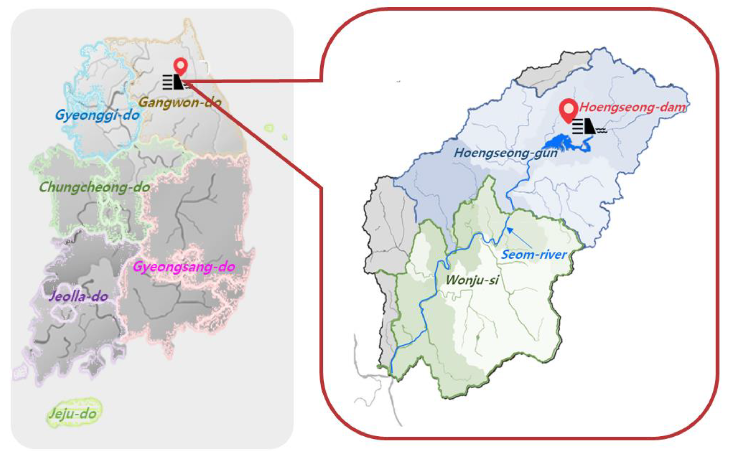
The Hoengseong multi-purpose dam (hereafter, H-dam), located in Gangwon-do, South Korea, was selected to demonstrate the developed model. Figure 1 shows the location of the dam, Seom-river and Hoengseong-gun and Wonju-si, which receive water from the dam. The construction of H-dam started in December 1993 and was completed in November 2000. Table 1 lists the specifications of the dam.
Before the construction of the H-dam, the middle and downstream areas of the Seom-river suffered considerable flood damage in the wet season and serious water shortages in the dry season. To address those problems, the dam was constructed in the Seom-river basin to supply water to small and medium-sized cities in the downstream areas, such as Hoengseong-gun and Wonju-si. The dam plays its role in preventing flood damage by securing a flood control capacity of approximately 9.5 million m3. The population of the area (Hoengseong-gun and Wonju-si) was approximately 370,000 in 2015 [21]. Agriculture and industry were developed in the area, and the dam supplies domestic, industrial, and agricultural water. Along with the construction of the H-dam, a water culture pavilion and a Hoengseong lake trail were created near the dam to provide local residents with recreational spaces. Additionally, the supply of maintenance water to the rivers in the downstream area improves the environment, water supply, and irrigation. The dam also reduces floods, thereby contributing to the stability and safety of residents.
Table 2 lists the statistic values of the study area in 2015, and the available data period. Note that the dam operation started in 2002 and the data related to the dam is only available after year 2002. The data used by the model were collected from the Water Supply Statistics [21], the Korean Statistical Information service [22], and the Water Management Information System [23].
2.2. System Dynamics Model Construction
2.2.1. System Dynamics
System dynamics is a research methodology developed by Forrester, an industrial engineering professor in the U.S., in 1961 [24]. This technique can be used to identify dynamic changes in an entire system with a focus on causal relationships and the feedback between system components. System dynamics has the following characteristics. First, it is not a single, one-way sequential line of events; instead, it reflects the interactive influence of feedback mechanisms [25]. Therefore, it is suitable for describing long-term changes in a target system, i.e., the future evolution and development processes of the system. Second, it finds the causes of changes in the system from the feedback structure. Because systems in modern society are complex, it is necessary to understand and analyze the feedback structure, which makes it possible to identify the causal relationships between components, rather than favoring one-way thinking [26].
System dynamics uses a causal loop diagram to describe the feedback structure. A causal loop diagram enables the visualization of causal relationships among the components that constitute the target system. A causal loop uses arrows to represent the relation and direction between elements, as well as (+) and (−) signs to indicate positive and negative correlations, respectively.
The modeling process uses system dynamics, which begins by defining the problem in the target system of interest. Next, various elements that constitute the target system are examined from a feedback perspective, and a causal loop is created to identify their causal relationships in the conceptualization phase [27]. A model can be constructed based on this phase, and long-term changes in the system are examined by simulating the target model through an appropriate scenario. In this study, we used Vensim DSS [28] to construct a model using the system dynamics technique. Vensim is the system dynamics simulation software developed by Ventana and is known to be useful in conceptualizing, designing, simulating, and analyzing complex systems [29].
2.2.2. Causal Loop
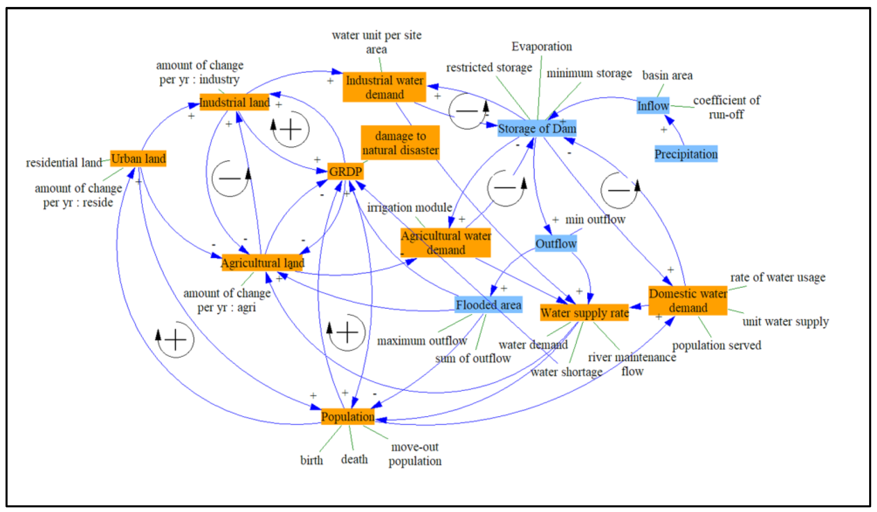
Figure 2 shows the causal relationships among the components of the developed model. An increase in population causes an increase in domestic water demand and urban land area (residential, commercial, and industrial land). The increase in urban land raises the demand for domestic and industrial water, but urban development in a limited land area causes a decrease in the agricultural area, thereby reducing agricultural water demand. An increase in industrial and decrease in agricultural land are related to the production per unit area, which affects GRDP. A growing GRDP reflects a growing economy, which attracts people to an urban area and increases the demand for urban land at the expense of agricultural land.
Precipitation affects dam inflow and outflow. Thus, large precipitation causes an increase in dam inflow and outflow. When precipitation is small, the water stored in the dam is inevitably used due to water shortage, which again affects the storage and outflow of the dam. Prior to the flood season between June and September, the dam is required to maintain space for flood control. During normal periods, its storage and outflow must be adjusted to supply sufficient water by means of dam operation and management, such as securing storage by adjusting the water level of the dam and determining outflow to ensure a stable water supply during the flood and non-flood periods of each year, respectively. A large outflow in the flood season could cause inundation in the downstream area, resulting in damage to crops, and thereby affecting agricultural output and GRDP. In addition, a lack of available water in the dry season affects agricultural production, which also decreases GRDP. Changes in GRDP reflect a regional economy, which potentially affects the population migration of the area.
Based on these causal relationships, relational equations between the elements of each system can be determined. Here, the historical data of the area can be used to estimate the relationships. For the hydro-sector, the flooded area was included and dam operation was simulated using dam elements, such as the actual storage, restricted storage, minimum storage, inflow, outflow, and precipitation. For the socio-sector, a model was constructed using the population, residential land, industrial land, agricultural land, GRDP, and amount of damage to crops due to natural disasters. The water demand for domestic, industrial, and agricultural areas is also included in the model. The relationships among those elements can be seen in Figure 2.
2.2.3. Sub-Modules of the Socio-System
The components of the socio-system are population, land use (residential, industrial, and agricultural), water demand for the domestic, industrial, and agricultural sectors, GRDP, flood damage, and water supply rate (a ratio of water supply to demand), as shown by the orange shaded terms in Figure 2. Representative components reflecting the characteristics of the target area were selected to analyze the quantitative change in each component caused by dam construction in the target basin. The relational formulas between components were estimated using historical data and their causal relationships. For model construction, we first analyzed the historical data of the elements to identify the temporal pattern of each element and correlations among the elements. Based on the data analysis results, we sketched the causal loop diagram. The relational formulas were then developed and applied to the causal loop diagram to quantify the relations among the elements. Finally, the model calibration was conducted by adjusting the parameters of the relational formulas to fit the simulation results to the historical data. In the constructed model, the elements can affect each other because they are connected in a feedback relationship that allows each element to change the other elements.
The population was calculated by accumulating the annual population increment or decrement from the base year (Equation (1)). The increment or decrement was calculated considering births, deaths, and the number of people moving in and out. In this case, the number of people moving in and out was calculated by considering changes in land use (residential and industrial area), changes in GRDP, and move-out due to the damage from natural disasters (floods or droughts) in the target area. In Equation (1), is the total population of year ; is the initial population in the first year of the simulation period , and is the net population increment or decrement in year .
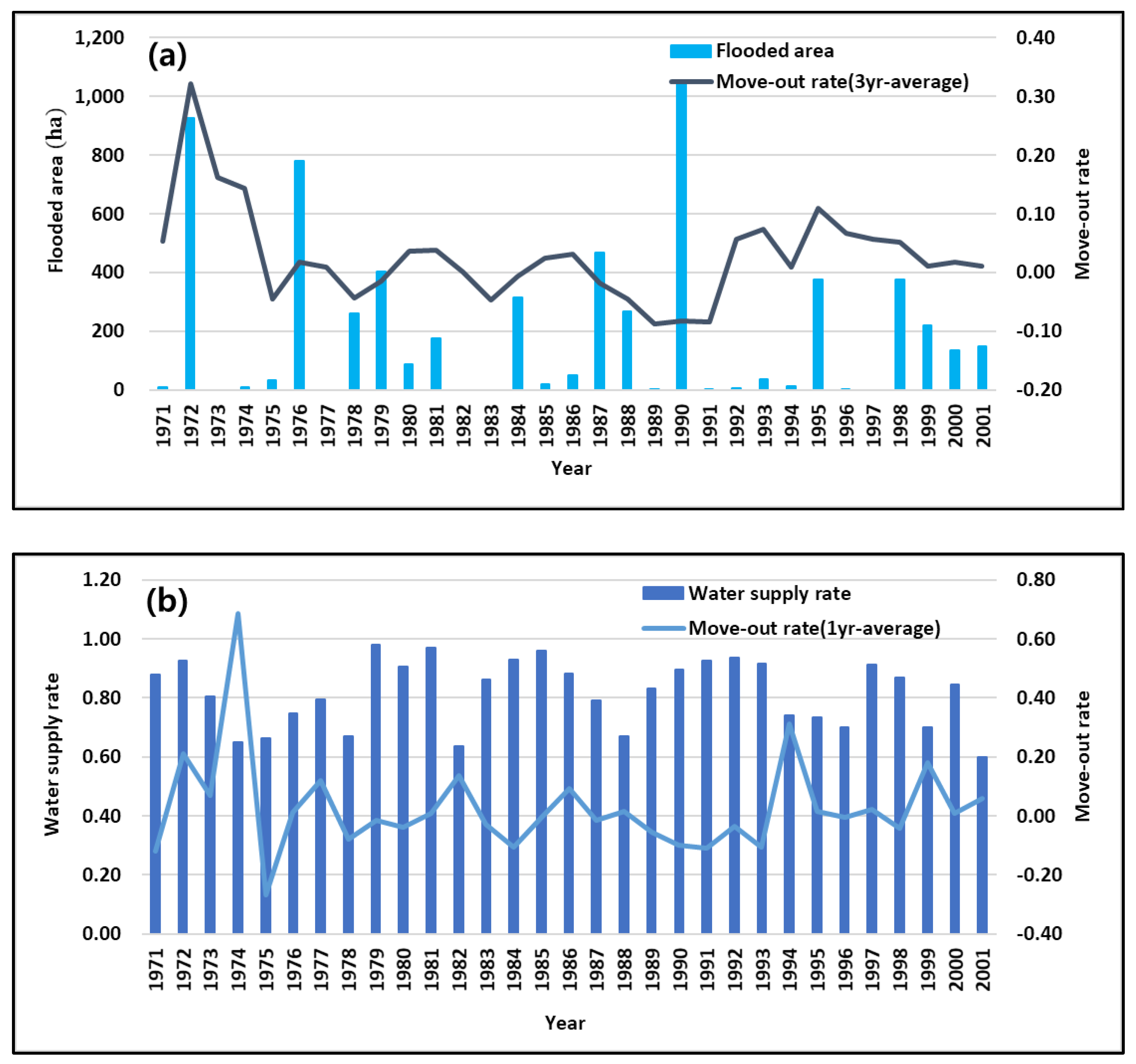
Figure 3a shows the flooded area and move-out rate of the target area in the past (1971–2001) due to flood damage. Based on these results, the relationship between the two variables can be identified. Figure 3b shows the relationship between the water supply rate and the move-out rate of the area in the past (1971–2001), which was plotted to analyze the relationship between water shortages and move-out rates. Flood damage was judged by the flooded area in Figure 3a, and drought damage was judged by the water shortage (=1—water supply rate) in Figure 3b The move-out rate represents the ratio of the average number of people who moved out in the following year(s) to the number of people who moved out in the corresponding year. In Figure 3, positive move-out rates indicate that the number of people who moved out of the area increased, thereby reducing the population calculation. In other words, they indicate that when natural disasters, such as floods and droughts, occurred in the area, the number of people who moved to other areas increased due to the experience of inundation, damage to crops, and water shortages.
The move-out population for three consecutive years after a disaster was analyzed to identify the relationship between damage and move-out rates. In the case of flood damage, the move-out population increased for up to three years after considerable inundation damage. In the case of drought (i.e., water shortage), the move-out population increased for a year any time the water supply rate dropped below 0.7. Figure 3a shows the flooded areas and the three-year average move-out rates, and Figure 3b illustrates the water supply rates and the one-year average move-out rates. These results reveal that some residents of the target area evacuated because they no longer considered it safe after they had experienced damage from flooding and drought. Therefore, population change could be estimated reasonably by analyzing the number of people who moved out due to natural disasters.
The net population change was calculated using Equation (2), where and are the number of births and deaths in year , respectively. is the industrial land change (km2/yr) in year and is the population density in the industrial area (person/km2). is the residential land change (km2/yr), and is the population density in the residential area (person/km2). is the GRDP change (KRW/yr) of the area, and is the population growth per GRDP increment (person/KRW). Note that 1 USD is equivalent to 1200 KRW. is the number of people who moved out due to the occurrence of flooding and drought. Thus, the population change is assumed to be affected by changes in land use, GRDP, and disaster occurrence in the target area.
Land use was classified into residential, industrial, and agricultural areas. The residential area was calculated using Equation (3), where, and are the residential land area (km2) in year and the first year of the simulation, respectively. is the population change (person/km2) in year , and is the reciprocal of (km2/person). is the GRDP change (KRW/yr) in the area, and is the residential land change per GRDP change (km2/KRW). is the agricultural land change (km2/yr), and is the residential land change due to the agricultural land change (km2/km2). is the industrial land change (km2), and is the residential land change due to the industrial land change (km2/km2). Thus, the changes in the residential area are affected by population, GRDP, and the land used for industry and agriculture.
Similarly, the industrial area was calculated using Equation (4) and is affected by population, GRDP, and land use for residences and agriculture. and are the industrial land area (km2) in year and the first year of the simulation, respectively. is the population change (person/yr), and is the reciprocal of (km2/person). is the GRDP change (KRW/yr) in the area, and is the industrial land change per GRDP change (km2/KRW). is the residential land change (km2/yr), and is the industrial land change due to the residential land change (km2/km2). is the agricultural land change (km2/yr), and is the industrial land change due to the agricultural land change (km2/km2).
Finally, agricultural land was calculated using Equation (5) and is affected by GRDP, land used for residences and industry, and the area damaged by flooding. and are the agricultural land area (km2) in year and the first year of the simulation, respectively. is the GRDP change (KRW/yr), and is the agricultural land change per GRDP change (km2/KRW). is the industrial land change (km2/yr), and is the agricultural land change due to the industrial land change (km2/km2). is the residential land change (km2/yr), and is the agricultural land change due to the residential land change (km2/km2). Moreover, is the flooding area in year and is calculated using Equation (6). Flooding damage frequently occurs in the flood season. Therefore, the flooded area, , was estimated using the total and maximum runoff in the flood season (June to September). A regression equation was estimated using historical runoff data and flood statistic values. Here, α and ß are the parameters for calculating the flooded area according to the total and maximum runoff, respectively. Prior to dam construction, and represent the total streamflow (m3) and maximum streamflow (m3/month), respectively, during the flood season. After dam construction, and represent the total and maximum dam outflow (m3), respectively, during the flood season.
GRDP is an economic index representing the value created by economic activities. It is affected by the population, industrial and agricultural production, and damage caused by flooding or drought and is calculated using Equation (7). is the GRDP (KRW) in year ; is the production per capita (KRW/person); is the production per industrial land area (KRW/km2), and is the production per agricultural land area (KRW/km2). Additionally, is the water shortage amount (m3) in year , and is the amount of water required per unit agricultural area (m3/km2). Thus, the fourth term in Equation (7) indicates the economic loss caused by water shortages in the agricultural area. indicates the flood damage amount and is estimated as the sum of runoff, maximum runoff, and flooded area during the flood season, as expressed in Equation (8). Here δ, ε, and ζ are the parameters for calculating the flood damage according to the total runoff, maximum runoff, and flooded area, respectively.
The water supply rate is quantitatively calculated to determine the water supply availability in the target area. Total water use includes domestic, industrial, and agricultural water consumption and river maintenance flow, and the water supply capacity includes the streamflow (before dam construction) or dam outflow (after dam construction). Therefore, the water supply rate is calculated as the ratio of the water supply capacity to the total water use, as expressed in Equation (9), where is the water supply rate; is the total water demand (m3), and is the water supply capacity in year . For agricultural water demand, it was assumed that 80% of the total demand would be evenly consumed during the irrigation period (April–September), with the remaining 20% evenly allocated to the non-irrigation period (October–March). The annual domestic and industrial water demand is evenly distributed over the 12 months regardless of the season.
is the water shortage (m3) in year , and is expressed as shown in Equation (10).
2.2.4. Sub-Modules of the Hydro-System
The blue blocks in Figure 2 indicate the components of the hydro-system: precipitation, dam (inflow, storage, outflow, evaporation), and river maintenance flow. The dam operation model for the simulation was constructed on a monthly basis. The monthly inflow into the dam was determined by the monthly precipitation and watershed information, and the dam storage and outflow were determined using the dam operation model.
The dam inflow was calculated using the monthly precipitation, dam basin area, and runoff coefficient, as expressed in Equation (11). is the dam inflow (m3/month) in month ; is the monthly rainfall (mm/month); is the basin area (km2), and is the runoff coefficient. Here, the dam outflow is adjusted according to the inflow and storage, as obtained through the monthly operation simulation.
In the dam operation model, the restricted storage and minimum storage were set considering the specifications of the dam. Minimum monthly outflow was set by analyzing the water demand and downstream river maintenance flow in the past. In particular, when the dam storage was insufficient in the dry season or when restricted water supply was required, the minimum outflow was adjusted according to the dam operation rule.
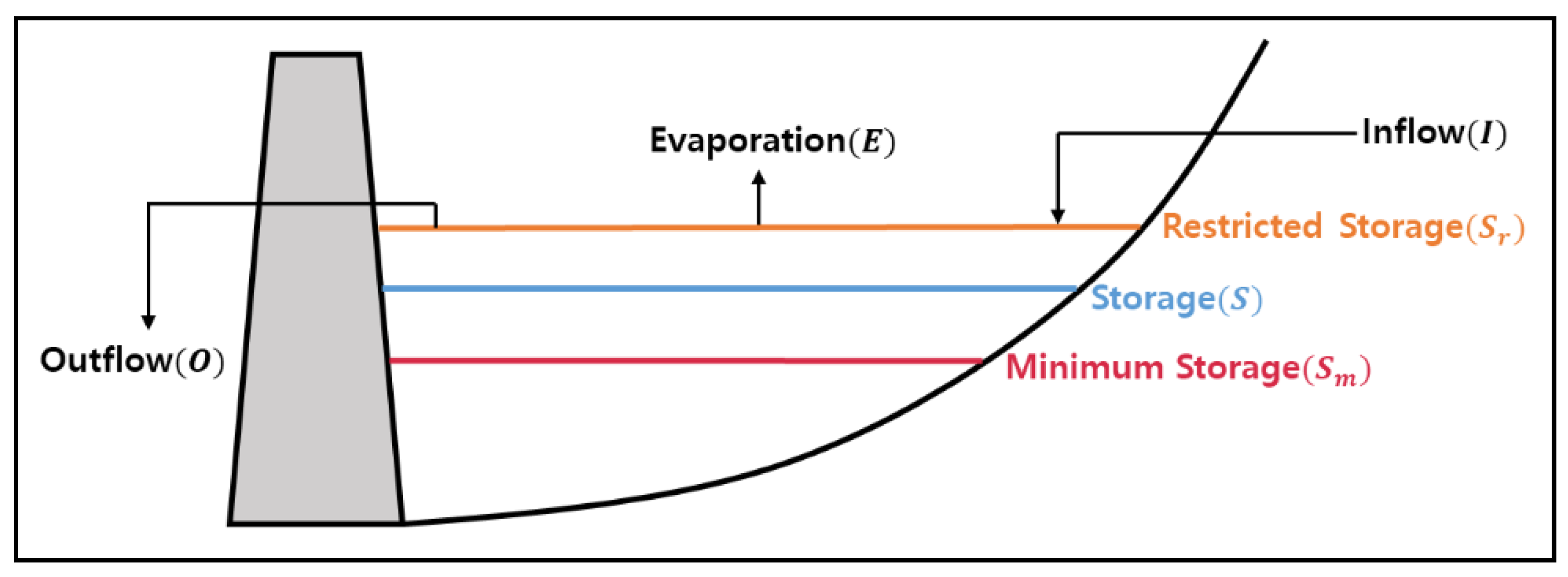
Equation (12) is a water-budget equation for a dam (Figure 4). Here, ) and are the water storage (m3) of the dam in months and , respectively. is the evaporation (m3), and is the outflow (m3) from the dam in month .
The outflow can be calculated for two cases. In the first case, when the inflow exceeds the restricted storage, the outflow is calculated using Equation (13). That is, the maximum value between the excess of the restricted storage and the minimum outflow is determined to be the outflow. Here, is the restricted storage (m3) in month , and is the predefined minimum outflow (m3).
In the second case, when the inflow fails to reach the restricted storage, the outflow is calculated using Equation (14). That is, the maximum value between 50% of the water quantity obtained by subtracting the evaporation from the inflow and the minimum outflow is determined to be the outflow.
Note that the minimum dam storage is specified, and the dam operation is simulated within the range of [minimum storage, restricted storage]. If downstream suffers flooding damages, the operators would increase the storage capacity to store more water in the dam; on the other hand, under severe droughts, the minimum outflow would be adjusted temporarily to secure water supply. In addition, if the downstream area requires more water due to urbanization, the minimum outflow would be increased (by changing the operation rules permanently) to supply the increased demand. In this way, the feedback from downstream can be reflected in the dam outflow in the model.
2.3. Scenario Development
In this study, we developed and simulated three plausible future scenarios, namely the baseline scenario, the extreme climate scenario, and the rapid urbanization scenario.
2.3.1. Baseline (Scenario 1)
The Representative Concentration Pathways (RCPs) describe four different 21st-century pathways of greenhouse gases and atmospheric concentrations, air pollutant emissions, and land use [30,31]. Comparing four pathways, we chose the RCP8.5 as a baseline because this scenario seems to represent the current conditions of the study site and plausible future condition. Note that the RCP8.5 indicates no specific climate change mitigation target in the area [32]. The projected annual rainfall data were obtained from the Korea Meteorological Administration, generated by multi-model ensemble means from the CMIP5 (e.g., more than 20 models) under the RCP 8.5 scenario [33].
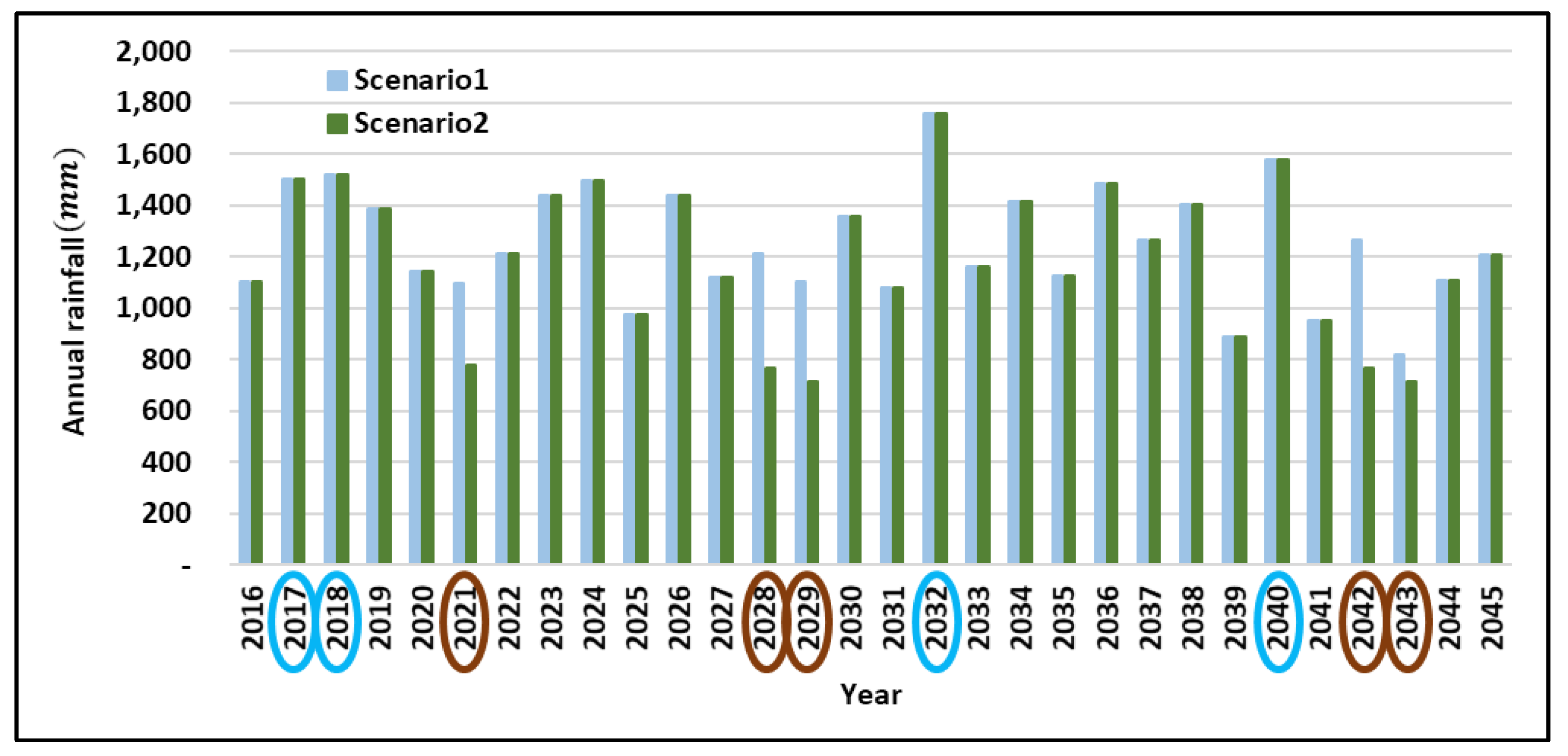
2.3.2. Extreme Climate (Scenario 2)
The extreme climate scenario, which is a modification of the Baseline scenario (Scenario 1), hypothetically generates drought and flood years by manipulating precipitation to observe changes in the social and hydrological components of the target area. Figure 5 shows the annual rainfall for the next 30 years in the extreme climate scenario compared with scenario 1. For years of 2017, 2018, 2032, and 2040 in blue circles, which correspond to flood years, the annual rainfalls are the same as scenario 1, but the monthly rainfalls in the flood season (June to September) were purposely increased to induce flood events. On the other hand, for years of 2021, 2028–2029, and 2042–2043 in brown circles, which correspond to drought years, the monthly rainfalls of the past drought events (2014–2015 drought) in the target area were applied. Note that the 2014–2015 drought was one of the worst droughts occurred in the target area.
2.3.3. Rapid Urbanization (Scenario 3)
For simulation of rapid urbanization in the target area, the following assumptions were made for the next 30 years: (1) higher-than-expected births, (2) an increase in water consumption per capita due to improved living standards, and (3) an increase in production per unit of industrial land due to technological developments. This simulation was conducted using the annual rainfall of the Baseline scenario with dam operation.
3. Results and Discussion
3.1. Model Calibration
To determine the applicability of the developed model for future scenarios, we first performed model calibration by comparing the statistical data with the simulation results of the model. The construction of the H-dam was completed in November 2000, and operations began in 2002. Therefore, the periods before and after dam construction were divided based on the year 2002. Table 3 summarizes the list of the parameters used for model calibration. The calibration was conducted using a trial-and-error, until the simulation results follow the trend of the historical data (visual inspection) and acceptable error is achieved by adjusting the parameters. Table 4 summarizes the overall root mean square error (RMSE) between the historical data and the simulation results.
3.1.1. Population
The calibration period was from 1965 to 2015, and the results are shown in Figure 6. The population of the target area in 1965 was approximately 240,000, which increased to approximately 370,000 by 2015. The population did not change significantly until the early 1990s and has slowly increased since the mid-1990s. It has increased continuously since the construction of the dam. Throughout the simulation period, the simulated values closely followed the statistical data.
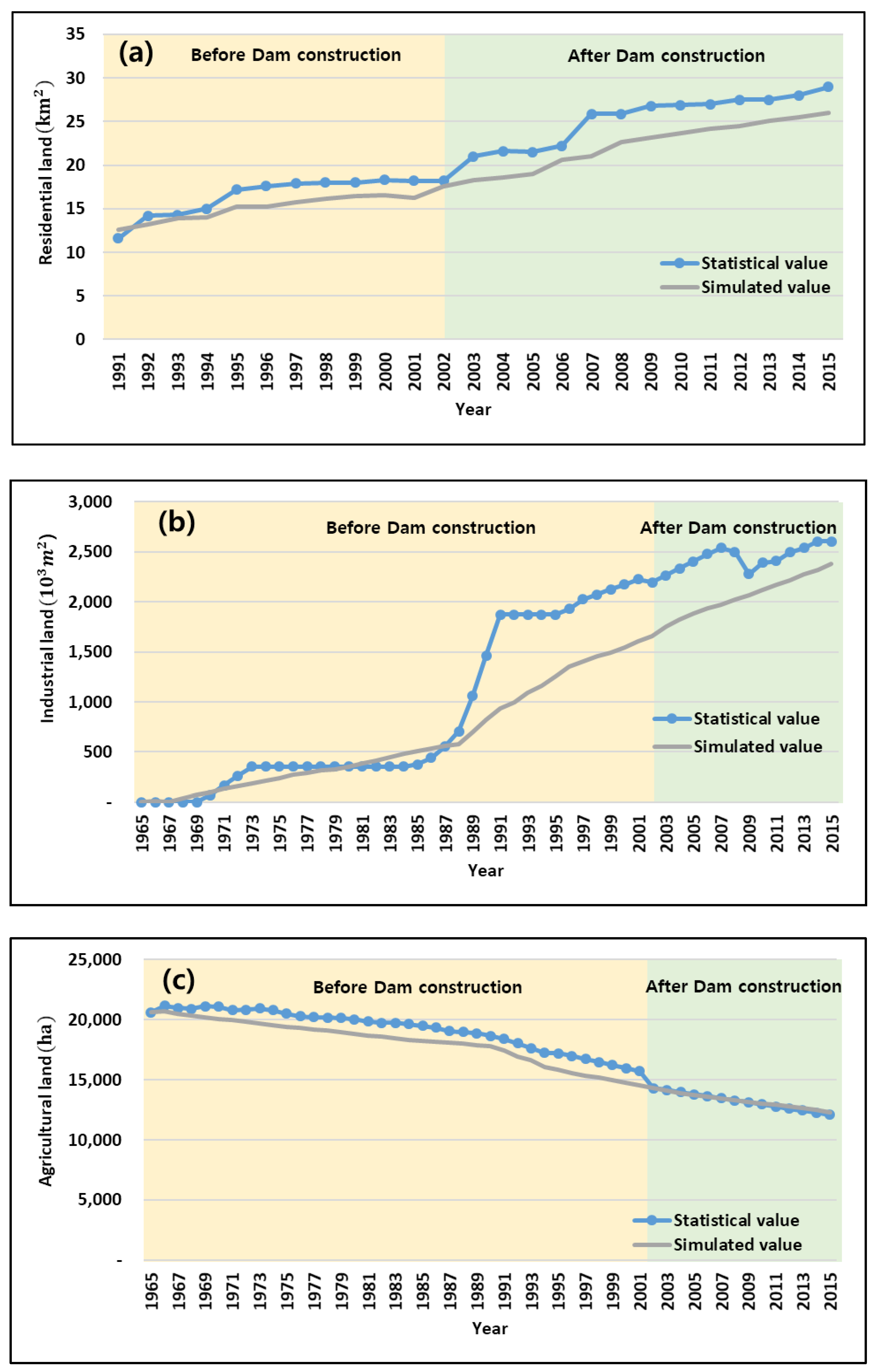
3.1.2. Land Use
The land use of the target area was divided into residential, industrial, and agricultural land. The calibration period for residential land was from 1991 to 2015 due to a lack of data, and that for industrial and agricultural land was from 1965 to 2015. Figure 7 shows the simulation results for each land-use type. For residential land (Figure 7a), the area has increased continuously since the 1990s, which is similar to the population change results. For industrial land (Figure 7b), the area sharply increased in the late 1980s due to the industrial development and a population influx. The developed model could not accurately reflect this sharp, rapid increase, but it did simulate the overall increasing trend. For agricultural land (Figure 7c), the area has decreased continuously, likely because of the conversion of farmland into residential and industrial land following urbanization and industrialization. The model accurately simulated this decreasing trend.
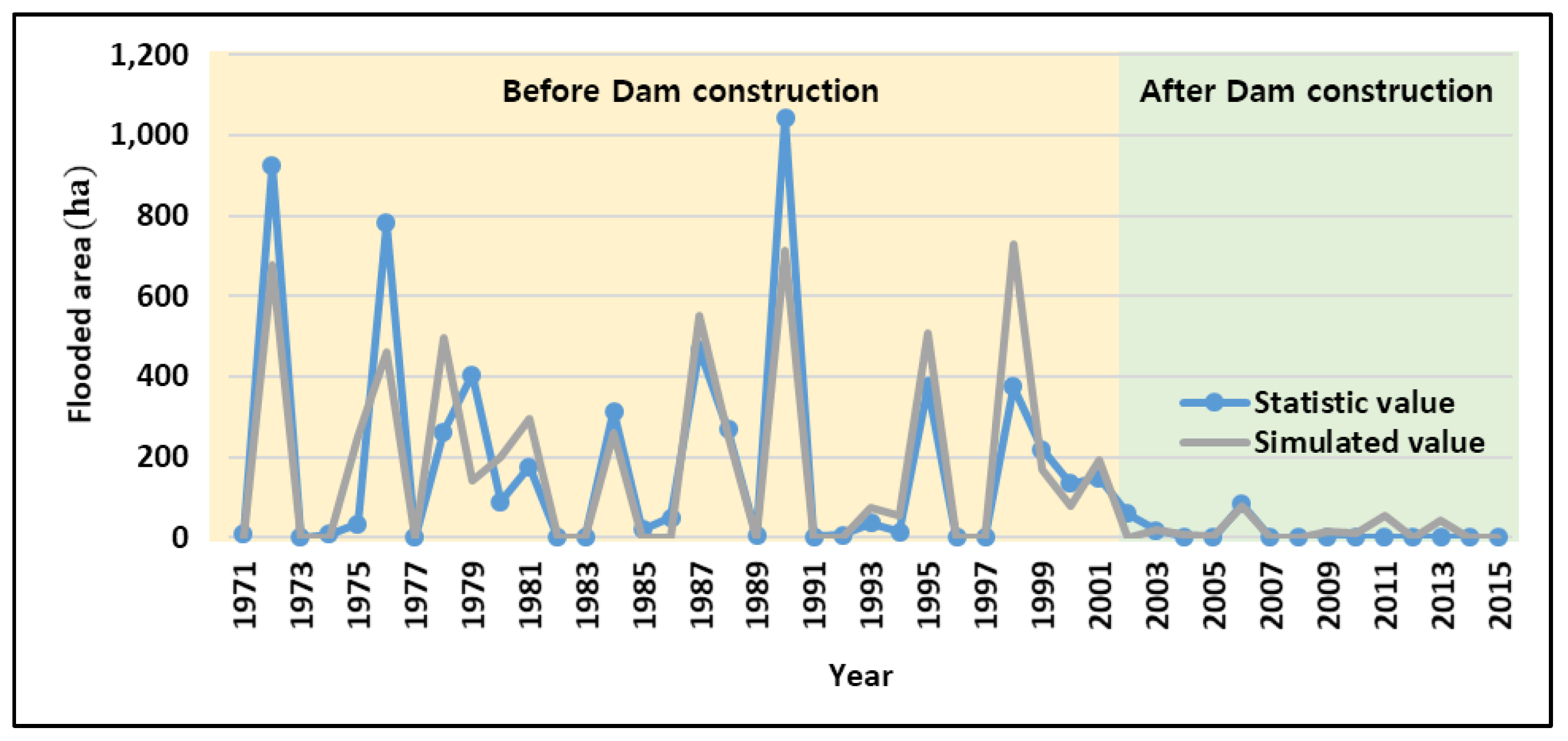
3.1.3. Flooded Area
The calibration period for the flooded area was 1971 to 2015, and the results are shown in Figure 8. As shown in the figure, the flooded area decreased significantly after dam construction, which directly exhibits the flood reduction effect of the dam. Although relatively large rainfall events occurred after dam construction, there was no large inundation damage in the area downstream of the dam due to its storage and outflow control. The dam simulation results also reflect this flood damage reduction effect.
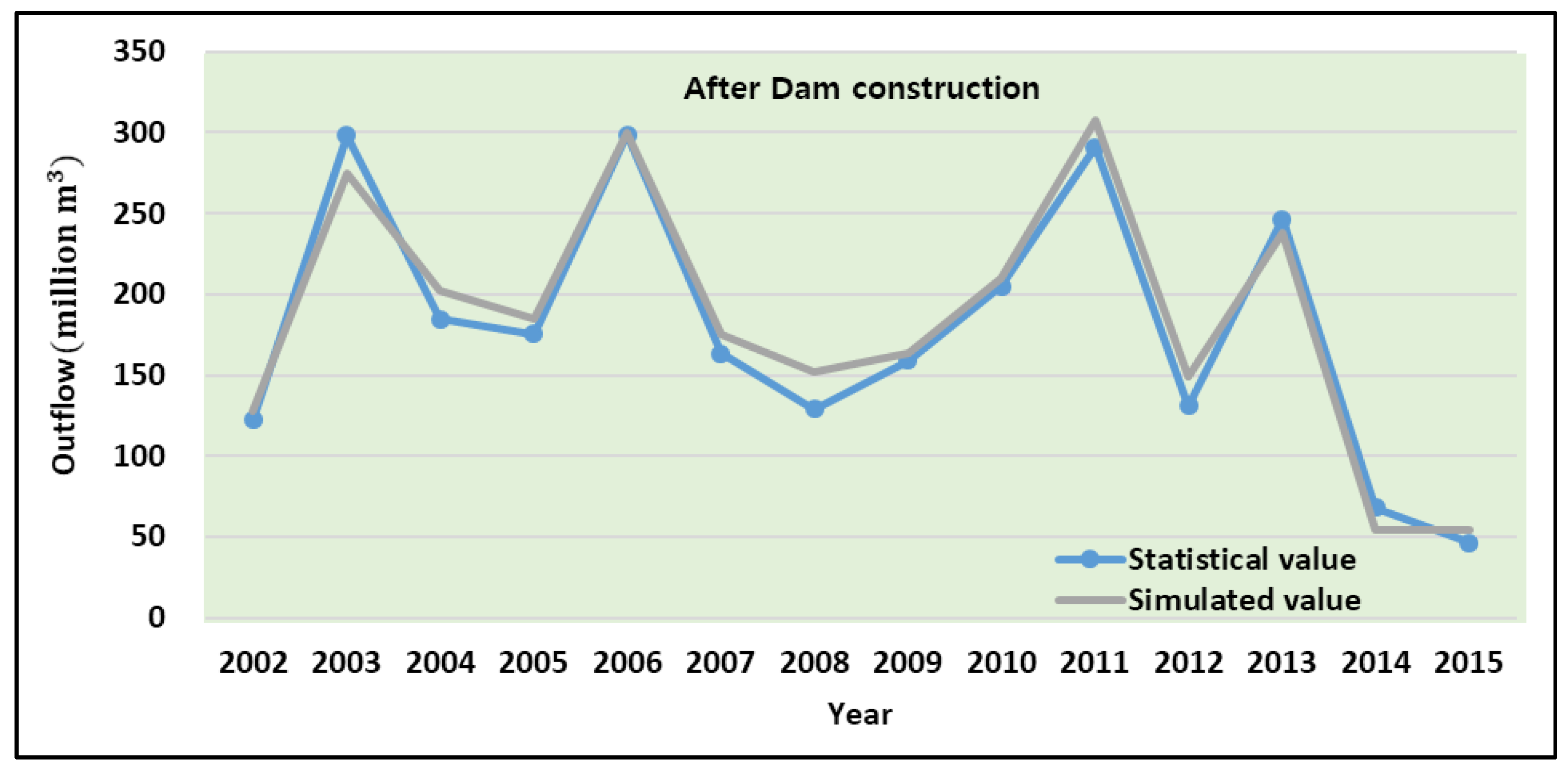
3.1.4. Dam Outflow
To calibrate the dam operation results, actual dam outflow data were compared with the simulated outflows. The calibration period was 2002 to 2015, and the results are shown in Figure 9. In the target basin, there were large differences in annual outflows between the years with large floods and those with severe drought. Overall, the simulated values are similar to the statistical data.
3.2. Scenario Analysis
3.2.1. Baseline (Scenario 1)
This scenario is a base scenario. Two simulations were performed, one on the assumption that the dam was constructed as it is now (With DAM) and the other that it was not constructed (Without DAM), and the results were compared and analyzed. From the comparison, the effects of dam construction on the target area were quantitatively estimated for the following four elements: population change, GRDP, inundation damage, and water supply rate. The future simulation period for the scenario was set to 30 years (2016–2045).
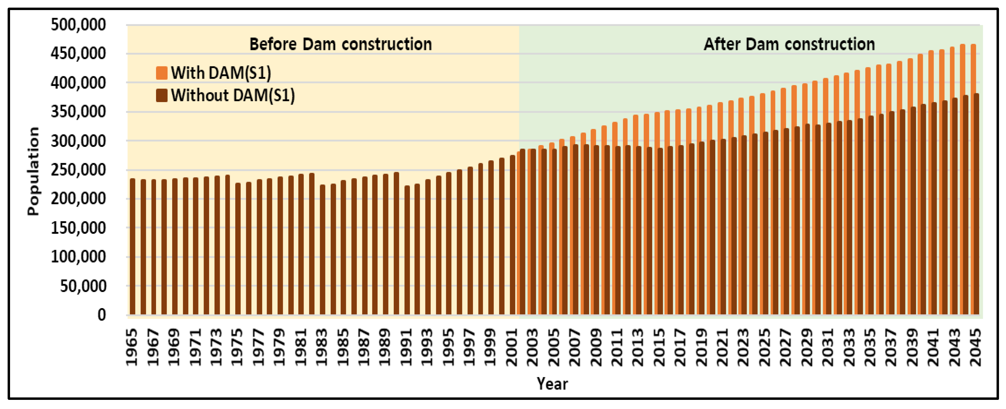
Population
In the simulation, the population was found to increase continuously following the previous trend. As can be seen in Figure 10, the case with dam construction (With DAM) exhibited a faster population increase than the case without dam construction (Without DAM). As of 2045, the population was estimated to be approximately 460,000 and 380,000 for the With DAM(S1) and Without DAM(S1) cases, respectively, resulting in a difference of approximately 80,000 people. Meanwhile, when the number of people who moved out during 30 years (2016–2045) was compared, With DAM(S1) exhibited approximately 10,000 fewer people than Without DAM(S1), apparently because efficient water resource management through the construction of the multi-purpose dam reduced the number of people who moved out of the target area by mitigating the damage caused by floods and droughts and inducing the activation of the regional economy. In the case without dam construction (Without DAM), the population increase in the target area was found to be slow due to an increase in the number of people moving out and slow regional development because of the future flooding and drought damages.
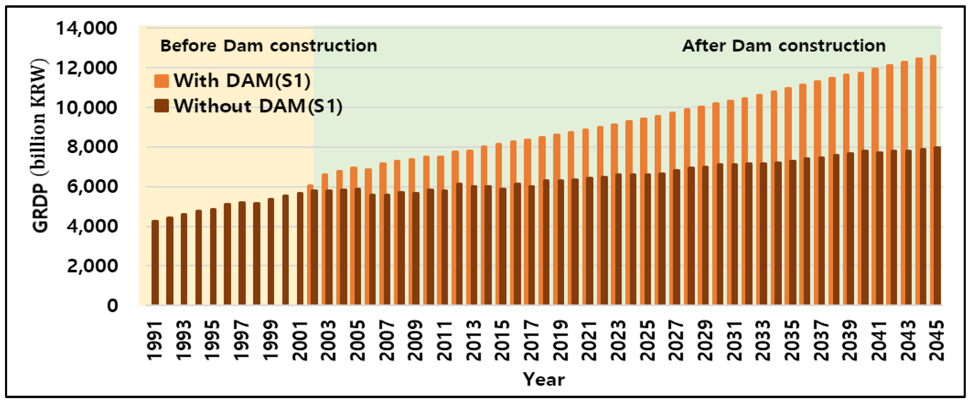
Gross Regional Domestic Product (GRDP)
Figure 11 shows the GRDP change patterns of the target area from 1991 to 2045. In the With DAM(S1) case, it was predicted that GRDP would consistently increase by approximately 150 billion KRW each year (on average) from approximately 7 trillion KRW in 2016 to 12 trillion KRW in 2045. In the Without DAM(S1) case, on the other hand, GRDP decreased in 2006 and 2011 when large flood damage occurred in the target area and again after 2014 and 2015 when severe drought damage occurred. From 2016, the GRDP of Without DAM(S1) is expected to increase by an average of approximately 60 billion KRW each year for 30 years. Thus, the average GRDP increment of With DAM(S1) is approximately 2.5 times larger than that of Without DAM(S1). By 2045, the GRDP of the Without DAM(S1) case is expected to be approximately 8 trillion KRW, about 4 trillion KRW lower than that in the With DAM(S1) case. In the developed model, GRDP was affected by population, industrial land, agricultural land, and damage by natural disasters. Therefore, the presence of the dam affected those variables, and they, in turn, affected GRDP. If the developed model is used in planning for a new dam, it will be possible to quantitatively analyze the future effects of dam construction on the economy of the target area.
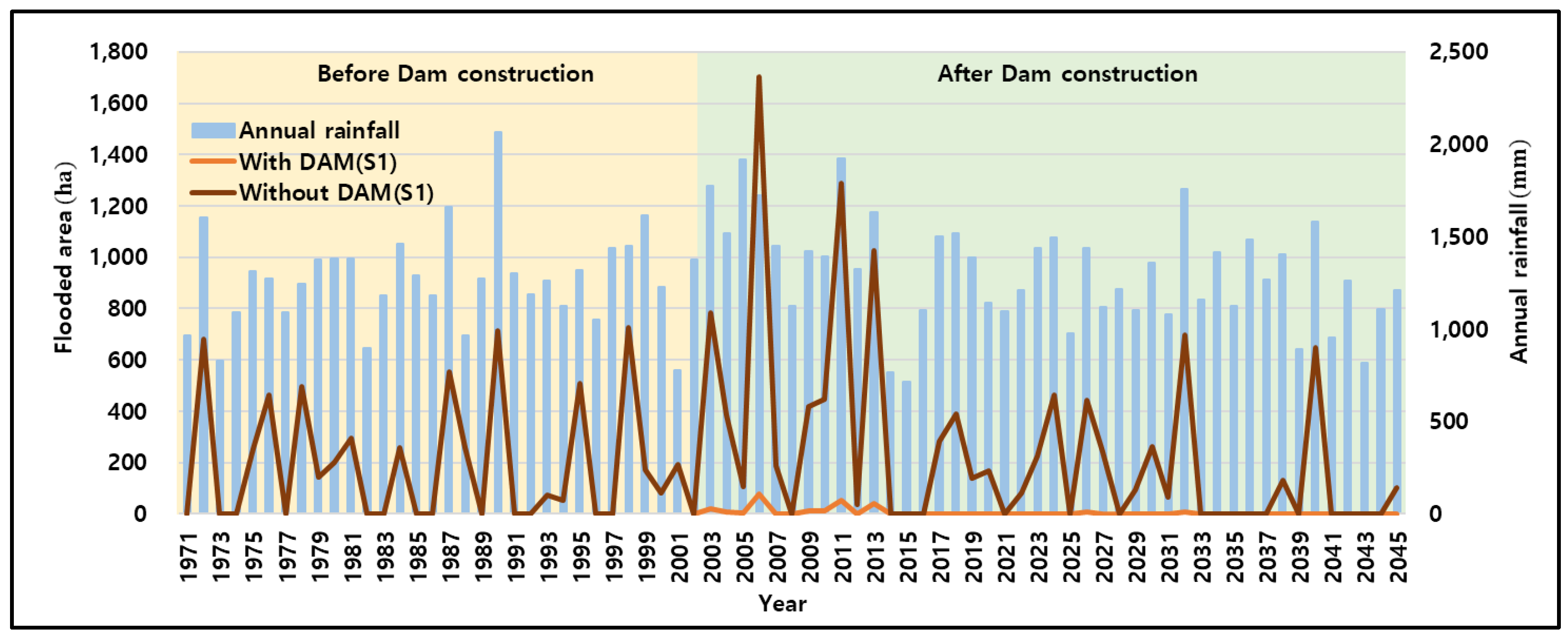
Flooded Area
The flooded area clearly shows the difference between the With DAM and Without DAM cases. As shown in Figure 12, approximately 4,500 ha of total inundation damage is expected to occur in the Without DAM(S1) case between 2016 and 2045, which corresponds to approximately 90 billion KRW when converted into a monetary value. For the With DAM(S1) case, however, almost no inundation damage (approximately 15 ha) is expected. The future inundation damage reduction through dam construction is expected to improve social values, such as economic vitality, by encouraging a population influx into the area and securing the land.
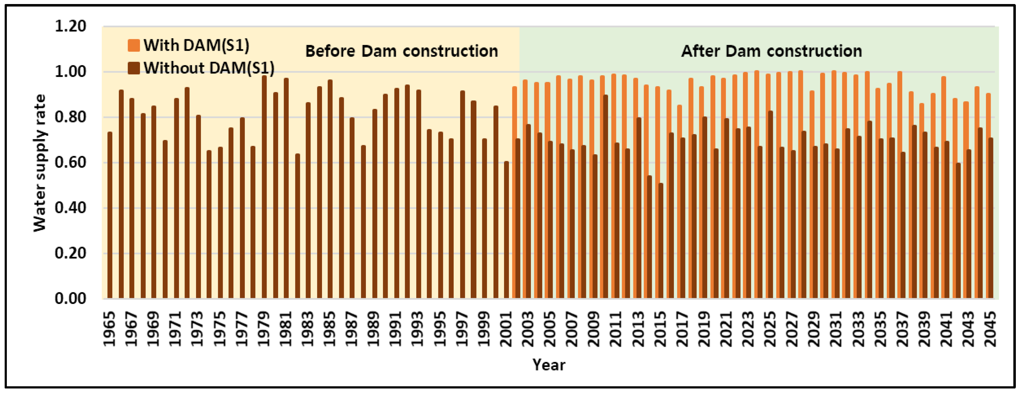
Water Supply Rate
Figure 13 shows the water supply rate for the target area from 1965 to 2045. The lowest water supply rate before dam construction was 0.61 in 2001, followed by 0.64 in 1982. The annual rainfall in 2001 was 780 mm, and that in 1982 was 900 mm, both significantly lower than the average annual rainfall for the area. Moreover, when the situations in 2014 and 2015, in which severe drought occurred in South Korea for two consecutive years, were simulated under the no-dam assumption, the water supply rates were calculated to be 0.56 and 0.51, and the annual rainfall amounts were found to be 765 and 717 mm, respectively. In the With DAM(S1) case during the same period, the actual water supply rates were 0.93 and 0.92, indicating that a stable water supply was possible.
The average annual water supply rate for 30 years (2016 to 2045) was calculated to be approximately 0.95 for With DAM(S1) and 0.71 for Without DAM(S1), indicating that water supply will be approximately 1.4 times more stable due to the dam construction.
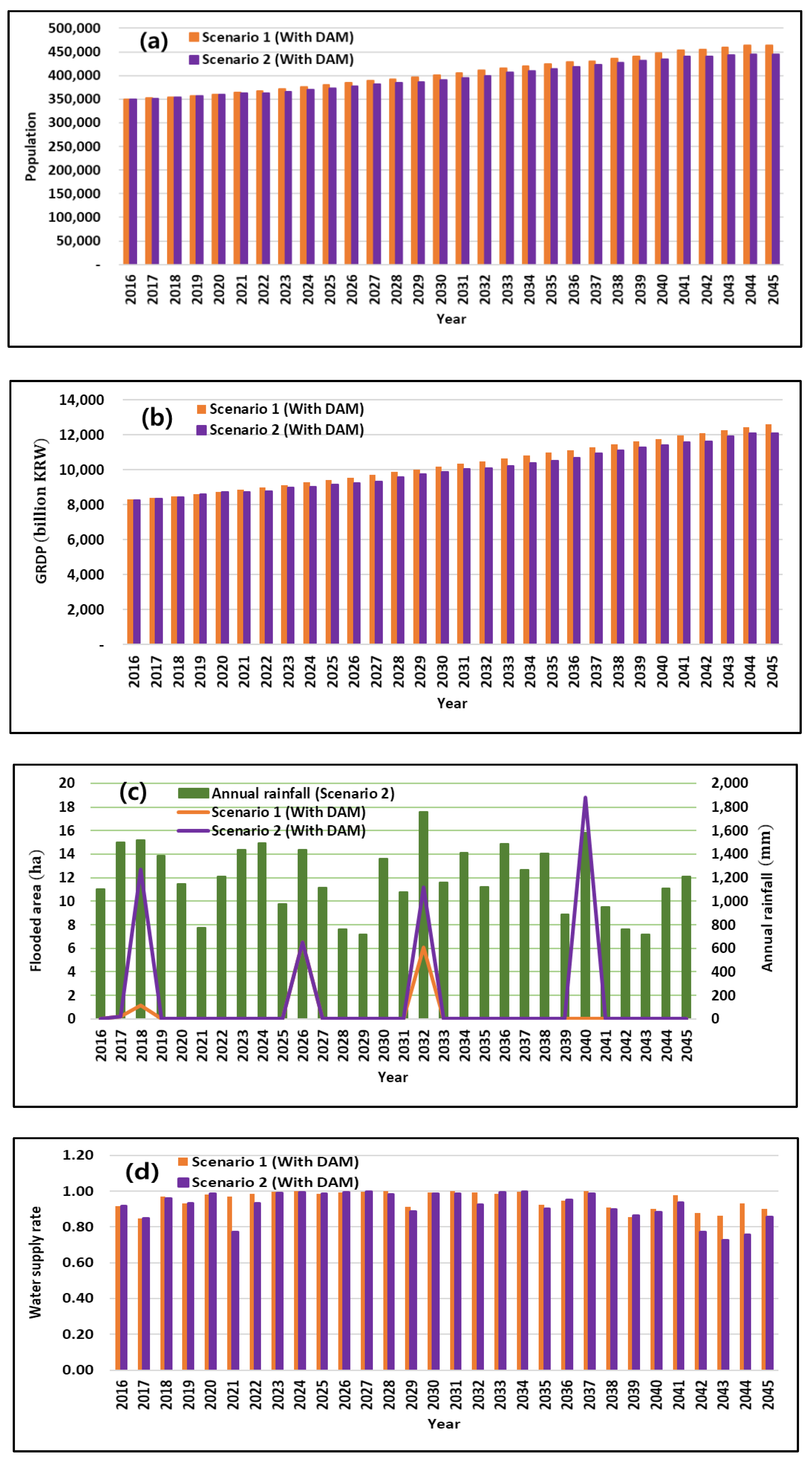
3.2.2. Extreme Climate (Scenario 2)
Figure 14 shows the results of the simulation performed for the target area with the dam for the next 30 years (2016–2045) using the RCP8.5 scenario (Scenario 1) and the extreme climate scenario (Scenario 2). The population simulation results in Figure 14a show that the population in 2045 will be approximately 460,000 in Scenario 1 and 440,000 in Scenario 2, for a difference of approximately 20,000 people. When the number of people who moved out during 30 years was compared, Scenario 2 had approximately 2000 more than Scenario 1. In Figure 14b, the GRDP simulation results exhibit patterns similar to those for population change. The GRDP in 2045 is expected to be approximately 12 and 11 trillion KRW for Scenarios 1 and 2, respectively, for a difference of approximately one trillion KRW. Figure 14c shows the flooded area simulation results. The total flooded area expected for the next 30 years was approximately 15 ha for Scenario 1 and 50 ha for Scenario 2, an insignificant difference. In other words, no large inundation damage is expected to occur because of the dam operation, even if large floods similar to those observed in the past occur in the target area in the future. Figure 14d shows the simulation results for the water supply rate during the next 30 years. The 30-year average water supply rate for Scenario 1 was approximately 0.95, and that for Scenario 2 was approximately 0.91, indicating that the water supply rate could be reduced by approximately 4% by extreme drought events. In the case of Scenario 2, the water supply rate for the three years from 2042 to 2044 dropped below 0.8 due to the occurrence of extreme drought for the two consecutive years of 2042 and 2043. These simulation results indicate that water shortages might occur if extreme drought occurs consecutively in the target area for a certain period, and therefore adequate preparation is required.
Based on the comparison of Scenarios 1 and 2, it is expected that future extreme climate events in the target area are unlikely to cause significant changes in the social and hydrological elements. In other words, massive damage caused by flooding or drought will probably not occur in the area if the dam is properly operated, and the population and GRDP is also expected to increase consistently.
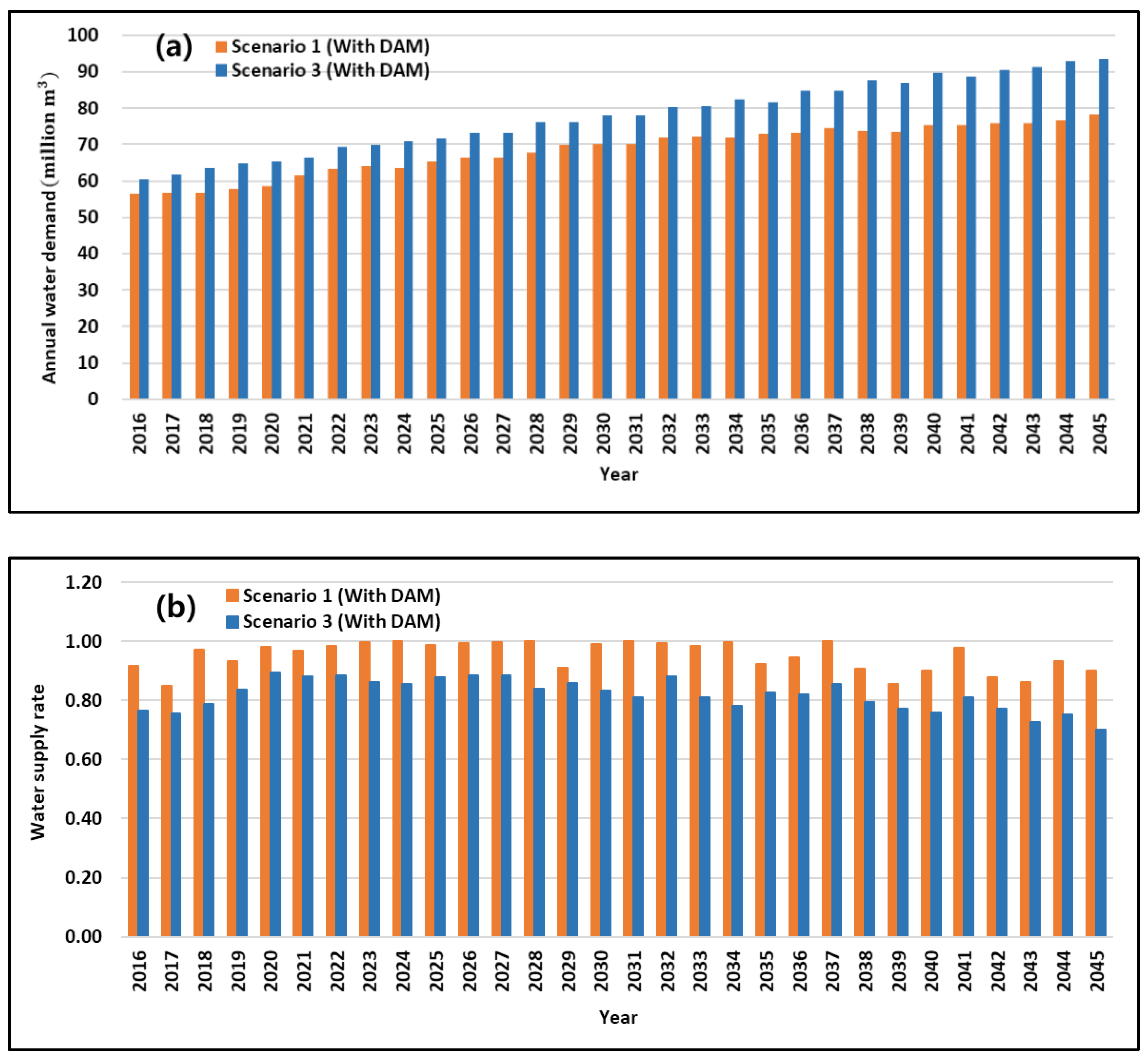
3.2.3. Rapid Urbanization (Scenario 3)
In Figure 15, the simulation results for total water use, which combines domestic, industrial, agricultural, and river maintenance flow, and the water supply rate are compared between Scenarios 1 and 3. The simulation results for Scenario 3 show that the GRDP increased higher than that of Scenario 1. The increased GRDP then accelerated the population influx into the area and caused the expansion of urban areas (residential and industrial), with a consequent reduction in agricultural land. Thus, the demand for domestic and industrial water soared, but the demand for agricultural water decreased. The target area receives most of its domestic and industrial water from the H-dam, whereas agricultural water is supplied from small-scale agricultural reservoirs scattered in the basin. Therefore, irrigation dependence on the H-dam is generally low.
As shown in Figure 15a, the total water uses in 2045 is expected to be approximately 78 million m3 in Scenario 1 and 95 million m3 in Scenario 3, for a difference of approximately 17 million m3. In Figure 15b, the average water supply rate in Scenario 3 is approximately 0.81, which is significantly lower than that for Scenario 1 (0.95). Thus, water supply shortages could occur if urbanization and industrialization progress faster than expected in the target area. Therefore, sustainable water management plans (e.g., water demand management, water reuse) should be established in conjunction with H-dam operation.
4. Conclusions
For multi-purpose dams, which are representative of large-scale water resource structures built for flood control and water supply, there is insufficient quantitative research on their effects on downstream areas. In this study, we developed a system dynamics model and used it under different scenarios to quantitatively analyze the effects of a multi-purpose dam on the population, economic change, response to disaster, and water supply in the downstream area. To apply the developed model, we selected the Hoengseong multi-purpose dam in Gangwon-do, South Korea. Prediction simulations were performed for the next 30 years (2016–2045), and the following conclusions were derived.
- 1.
- For Scenario 1, two case simulations were performed, one assuming dam construction (With DAM) and the other assuming no dam construction (Without DAM), and the results were compared to analyze the effects of the Hoengseong dam on the downstream area. When changes for the next 30 years were simulated, the population and GRDP were predicted to increase by approximately 80,000 and four trillion KRW, respectively, as of 2045 due to the 2002 completion of the Hoengseong dam. Furthermore, the flooded area will decrease by approximately 4480 ha, and the water supply rate will increase by approximately 1.4 times.
- 2.
- Scenario 2 simulated flood and drought years to analyze the effects of future climate changes in the target area. When Scenarios 1 and 2 were compared and analyzed from 2016 to 2045, it was concluded that future extreme climate events in the target area would not cause significant changes to social and hydrological elements. It appeared that no massive damage caused by flooding or drought would occur in the area, and the population and GRDP were expected to increase consistently.
- 3.
- Scenario 3 assumed increases in births, water consumption per capita, and production per unit of industrial land in the target area. The total water use, including domestic and industrial water, was expected to increase due to urbanization and economic revitalization. The 30-year average water supply rate dropped significantly; thus, water security plans would be required in conjunction with efficient dam operations.
In this study, we developed a system dynamics model to examine the effects of a multi-purpose dam on socio-economic factors of the downstream area. The model can be used as a decision-making tool to present grounds for engineering decisions and assist policymakers in planning and constructing a new multi-purpose dam. We also expect that the model can be adapted to perform effectiveness analyses and planning for other water resource facilities in the future.
Author Contributions
Conceptualization, D.K.; data curation, S.L.; formal analysis, S.L.; methodology, D.K. and S.L.; software, S.L.; supervision, D.K.; writing—original draft, S.L.; writing—review and editing, D.K. All authors have read and agreed to the published version of the manuscript.
Funding
This work was financially supported by the Korea Ministry of Environment (MOE) as a “Graduate School specialized in Climate Change”.
Conflicts of Interest
The authors have no conflicts of interest to declare.
References
- Sterman, J.D. Business Dynamics, Systems Thinking and Modeling for a Complex World; McGraw-Hill: Boston, MA, USA, 2000. [Google Scholar]
- Xu, Z.X.; Takeuchi, K.; Ishidaira, H.; Zhang, X.W. Sustainability analysis for Yellow River water resources using the system dynamics approach. Water Resour. Manag. 2002, 16, 239–261. [Google Scholar] [CrossRef]
- Zomorodian, M.; Lai, S.H.; Homayounfar, M.; Ibrahim, S.; Fatemi, S.E.; El-Shafie, A. The state-of-the-art system dynamics application in integrated water resources modeling. J. Environ. Manag. 2018, 227, 294–304. [Google Scholar] [CrossRef] [PubMed]
- Wei, S.; Yang, H.; Song, J.; Abbaspour, K.C.; Xu, Z. System dynamics simulation model for assessing socio-economic impacts of different levels of environmental flow allocation in the Weihe River Basin, China. Eur. J. Oper. Res. 2012, 221, 248–262. [Google Scholar] [CrossRef]
- Park, S.W.; Lee, T.G.; Kim, B.J.; Kim, T.Y. Development of a System Dynamics Model for the Efficient Operation and Maintenance of Sewerage Systems. J. Korea Water Resour. Assoc. 2012, 45, 101–111. [Google Scholar] [CrossRef]
- Ahmad, S.; Simonovic, S.P. System dynamics modeling of reservoir operations for flood management. J. Comput. Civil Eng. 2000, 14, 190–198. [Google Scholar] [CrossRef]
- Simonovic, S.P. Managing Water Resources: Methods and Tools for a Systems Approach; UNESCO: Paris, France; Earthscan James & James: London, UK, 2009. [Google Scholar]
- Kim, Y.J.; Jeong, E.S. Socio-hydrology or Hydro-sociology: Study on the co-evolution between human and the water cycle. Water Future 2015, 48, 34–43. [Google Scholar]
- Li, L.; Simonovic, S.P. System dynamics model for predicting floods from snowmelt in North American prairie watersheds. Hydrol. Process. 2002, 16, 2645–2666. [Google Scholar] [CrossRef]
- Simonovic, S.P. World water dynamics: Global modeling of water resources. J. Environ. Manag. 2002, 66, 249–267. [Google Scholar] [CrossRef]
- Stave, K.A. A system dynamics model to facilitate public understanding of water management options in Las Vegas, Nevada. J. Environ. Manag. 2003, 67, 303–313. [Google Scholar] [CrossRef]
- Simonovic, S.P.; Rajasekaram, V. Integrated analyses of Canada’s water resources: A system dynamics approach. Can. Water Resour. J./Revue Can. des Ressour. Hydr. 2004, 29, 223–250. [Google Scholar] [CrossRef]
- Neto, A.D.C.L.; Legey, L.F.; González-Araya, M.C.; Jablonski, S. A system dynamics model for the environmental management of the Sepetiba Bay watershed, Brazil. Environ. Manag. 2006, 38, 879–888. [Google Scholar] [CrossRef] [PubMed]
- Madani, K.; Mariño, M.A. System dynamics analysis for managing Iran’s Zayandeh-Rud river basin. Water Resour. Manag. 2009, 23, 2163–2187. [Google Scholar] [CrossRef]
- Khan, S.; Yufeng, L.; Ahmad, A. Analysing complex behaviour of hydrological systems through a system dynamics approach. Environ. Model. Softw. 2009, 24, 1363–1372. [Google Scholar] [CrossRef]
- Davies, E.G.; Simonovic, S.P. Global water resources modeling with an integrated model of the social–economic–environmental system. Adv. Water Resour. 2011, 34, 684–700. [Google Scholar] [CrossRef]
- Gaupp, F.; Hall, J.; Dadson, S. The role of storage capacity in coping with intra-and inter-annual water variability in large river basins. Environ. Res. Lett. 2015, 10, 125001. [Google Scholar] [CrossRef]
- Di Baldassarre, G.; Wanders, N.; AghaKouchak, A.; Kuil, L.; Rangecroft, S.; Veldkamp, T.I.; Van Loon, A.F. Water shortages worsened by reservoir effects. Nat. Sustain. 2018, 1, 617–622. [Google Scholar] [CrossRef]
- Wang, K.; Davies, E.G.; Liu, J. Integrated water resources management and modeling: A case study of Bow river basin, Canada. J. Clean. Prod. 2019, 240, 118242. [Google Scholar] [CrossRef]
- Park, S.W.; Kim, K.L.; Kim, B.J.; Lim, K.Y. Development of a System Dynamics Model to Support the Decision Making Processes in the Operation and Management of Water Supply Systems. J. Korea Water Resour. Assoc. 2010, 43, 609–623. [Google Scholar] [CrossRef] [Green Version]
- Ministry of Environment. 2016 Water Supply Statistics; Ministry of Environment: Sejong-si, Korea, 2018. [Google Scholar]
- Korean Statistical Information Service (KOSIS). Available online: http://kosis.kr/ (accessed on 8 April 2020).
- Water Management Information System (WAMIS). Available online: http://wamis.go.kr/ (accessed on 8 April 2020).
- Forrester, J. Industrial Dynamics; The MIT Press: Cambridge, MA, USA; Wiley: New York, NY, USA, 1961. [Google Scholar]
- Hjorth, P.; Bagheri, A. Navigating towards sustainable development: A system dynamics approach. Futures 2006, 38, 74–92. [Google Scholar] [CrossRef]
- Jung, S.H.; Joo, Y.J. A Study on the Analysis of Policy Effects for System Dynamics Methodology: Focusing on the sex trade special law. Korean Assoc. Public Adm. 2005, 39, 219–236. [Google Scholar]
- Jeong, H.S. Modeling Socio-Hydrological Systems for Wastewater Reused Watersheds. Ph.D. Thesis, The Graduate School Seoul National University, Seoul, Korea, 2014. [Google Scholar]
- Ventana Systems. Vensim User’s Guide Version 6; VENTANA Systems Inc.: Harvard, MA, USA, 2013. [Google Scholar]
- Kim, K.C.; Jung, K.Y.; Kim, S.W. SYSTEM DYNAMICS Using Vensim; Seoul Economic Management Publisher: Seoul, Korea, 2014. [Google Scholar]
- IPCC. Summary for Policy makers. In Climate Change 2013: The Physical Science Basis. Contribution of Working Group I to the Fifth Assessment Report of the Intergovernmental Panel on Climate Change; Cambridge University Press: Cambridge, UK; New York, NY, USA, 2013. [Google Scholar]
- Pachauri, R.K.; Allen, M.R.; Barros, V.R.; Broome, J.; Cramer, W.; Christ, R.; Dubash, N.K. Climate Change 2014: Synthesis Report. Contribution of Working Groups I, II and III to the Fifth Assessment Report of the Intergovernmental Panel on Climate Change (p. 151); IPCC: Geneva, Switzerland, 2014. [Google Scholar]
- Riahi, K.; Rao, S.; Krey, V.; Cho, C.; Chirkov, V.; Fischer, G.; Rafaj, P. RCP 8.5—A scenario of comparatively high greenhouse gas emissions. Clim. Chang. 2011, 109, 33. [Google Scholar] [CrossRef] [Green Version]
- Korea Meteorological Administration (KMA). Available online: https://www.weather.go.kr/ (accessed on 8 April 2020).
Figure 1.
Location of the Hoengseong multi-purpose dam.

Figure 2.
Schematic diagram of the causal loop in the proposed system dynamics model. The socio- and hydro-elements are represented in orange and blue, respectively.
Figure 2.
Schematic diagram of the causal loop in the proposed system dynamics model. The socio- and hydro-elements are represented in orange and blue, respectively.

Figure 3.
Relationship between natural disaster occurrence and the move-out rate (a) Flooded area, and (b) Water supply rate.
Figure 3.
Relationship between natural disaster occurrence and the move-out rate (a) Flooded area, and (b) Water supply rate.

Figure 4.
Dam water-budget analysis.

Figure 5.
Annual rainfall with scenarios 1 and 2 (blue circle indicates flood years and brown circle indicates drought years).
Figure 5.
Annual rainfall with scenarios 1 and 2 (blue circle indicates flood years and brown circle indicates drought years).

Figure 6.
Calibration results—population.

Figure 7.
Calibration results—land use (a) residential land, (b) industrial land, and (c) agricultural land.
Figure 7.
Calibration results—land use (a) residential land, (b) industrial land, and (c) agricultural land.

Figure 8.
Calibration results—Flooded area.

Figure 9.
Calibration results—dam outflow.

Figure 10.
Population comparison between the With DAM and Without DAM simulations for Scenario 1.

Figure 11.
Gross regional domestic product (GRDP) comparison between the With DAM and Without DAM simulations for Scenario 1.
Figure 11.
Gross regional domestic product (GRDP) comparison between the With DAM and Without DAM simulations for Scenario 1.

Figure 12.
Flooded area comparison between the With DAM and Without DAM simulations for Scenario 1.

Figure 13.
Water supply rate comparison between the With DAM and Without DAM simulations for Scenario 1.
Figure 13.
Water supply rate comparison between the With DAM and Without DAM simulations for Scenario 1.

Figure 14.
Comparison of Scenarios 1 and 2 for (a) population, (b) gross regional domestic product (GRDP), (c) flooded area, and (d) water supply rate.
Figure 14.
Comparison of Scenarios 1 and 2 for (a) population, (b) gross regional domestic product (GRDP), (c) flooded area, and (d) water supply rate.

Figure 15.
Comparison of Scenarios 1 and 3 for (a) Annual water demand and (b) Water supply rate.


Table 1.
Specifications of the Hoengseong multi-purpose dam.
| Height | 48.5 |
| Length | 205.0 |
| Basin area | 209.0 |
| Designed flood level | 180.0 |
| Restricted water level | 178.2 |
| Low water level | 160.0 |
| Total storage capacity | 86.9 |
| Effective storage capacity | 73.4 |
Table 2.
Statistics of the study area.
| Element | Value in 2015 | Available Data Period |
|---|---|---|
| Population | 370,000 | 1965–2015 |
| Residential land | 29.0 | 1991–2015 |
| Industrial land | 2.6 | 1965–2015 |
| Agricultural land | 121.0 | 1965–2015 |
| GRDP (billion KRW) | 8,600 | 1991–2015 |
| Annual rainfall | 717 | 1965–2015 |
| Annual water use | 59 | 1965–2015 |
GRDP = gross regional domestic product
Table 3.
Model calibration parameters.
| Element | Parameter | Description | Unit |
|---|---|---|---|
| Population | population density in the industrial area | person/km2 | |
| population density in the residential area | person/km2 | ||
| population growth per GRDP increment | person/KRW | ||
| Residential area | residential land change per population change | km2/person | |
| residential land change per GRDP increment | km2/KRW | ||
| residential land change due to the agricultural land change | km2/km2 | ||
| residential land change due to the industrial land change | km2/km2 | ||
| Industrial area | industrial land change per population change | km2/person | |
| industrial land change per GRDP increment | km2/KRW | ||
| industrial land change due to the residential land change | km2/km2 | ||
| industrial land change due to the agricultural land change | km2/km2 | ||
| Agricultural area | agricultural land change per GRDP increment | km2/KRW | |
| agricultural land change due to the industrial land change | km2/km2 | ||
| agricultural land change due to the residential land change | km2/km2 | ||
| Flooded area | regression parameter for total runoff | - | |
| regression parameter for maximum runoff | - | ||
| GRDP | production per capita | KRW/person | |
| production per industrial land area | KRW/km2 | ||
| production per agricultural land area | KRW/km2 | ||
| Dam operation | Runoff coefficient | - | |
| Evaporation | m3/month |
Table 4.
Calibration error root mean square error (RMSE).
| Element | RMSE | Unit |
|---|---|---|
| Population | 2095 | person |
| Residential land | 2.24 | km2 |
| Industrial land | 0.18 | km2 |
| Agricultural land | 1.30 | km2 |
| Flooded area | 0.18 | km2 |
| Dam outflow | 4.4 | million m3 |
© 2020 by the authors. Licensee MDPI, Basel, Switzerland. This article is an open access article distributed under the terms and conditions of the Creative Commons Attribution (CC BY) license (http://creativecommons.org/licenses/by/4.0/).
Share and Cite
MDPI and ACS Style
Lee, S.; Kang, D. Analyzing the Effectiveness of a Multi-Purpose Dam Using a System Dynamics Model. Water 2020, 12, 1062. https://doi.org/10.3390/w12041062
AMA Style
Lee S, Kang D. Analyzing the Effectiveness of a Multi-Purpose Dam Using a System Dynamics Model. Water. 2020; 12(4):1062. https://doi.org/10.3390/w12041062
Chicago/Turabian StyleLee, Sleemin, and Doosun Kang. 2020. "Analyzing the Effectiveness of a Multi-Purpose Dam Using a System Dynamics Model" Water 12, no. 4: 1062. https://doi.org/10.3390/w12041062
Note that from the first issue of 2016, this journal uses article numbers instead of page numbers. See further details here.