Controlled Reservoir Drawdown—Challenges for Sediment Management and Integrative Monitoring: An Austrian Case Study—Part B: Local Scale

Abstract

The present case study deals with a controlled drawdown beyond the operational level of the Gepatsch reservoir (Austria). Based on the awareness of potential ecological consequences, an advanced set of measures was conducted and an integrative monitoring design was implemented. This pre- and post-event monitoring included measurements regarding the cross sectional variability and habitat-related turbidity, freeze-core sampling to obtain knowledge on fine sediment infiltration and an evaluation of the macroinvertebrate communities as well as fish egg development (salmonid incubation). The results of the sedimentological as well as biological investigations show a negligible impact on the downstream located aquatic system due to the controlled drawdown of the Gepatsch reservoir. In addition, recommendations based on the findings from this study regarding possible methods for local scale monitoring can be given.

1. Introduction

The construction of hydropower plants and their operation affects the aquatic ecology on various scales [1]. Negative impacts on reproduction, growth and total biomass through different operation schemes like hydropeaking [2,3]; an interruption of migration corridors through weirs [4]; or a flow abstraction [5] are documented and also combined effects need to be considered [6]. More recently, sediment management actions in terms of preserving storage volume of reservoirs (e.g., mainly for energy production) were studied, which may result in additional negative impacts on aquatic organisms, like reduced macroinvertebrate communities [7], hypoxia of fish [8] and mechanical damage of fish (like gills) [9]. However, all these mentioned impacts happen during a limited period. In the long term, also changes on the downstream morphology, sediment quality and sediment quantity may influence the habitat quality permanently. In order to get better insight into possible negative impacts, in principle reach as well as at a local scale, aspects should be studied. In contrast to reach scale assessment (compare to [10]), local scale studies in terms of sediment management for controlled drawdowns or reservoir flushings were more frequently applied [7]. Especially, the increased fine sediment loads, which may follow controlled reservoir drawdowns or reservoir flushing, were investigated on a local scale; e.g., [9].

Monitoring strategies are mostly based on the Before-After-Control-Impact (BACI) approach [11,12]. Different abiotic and biotic parameters are used to document possible impacts on a local scale. For evaluating changes of the abiotic environment, measurements of fine sediment infiltration (FSI) and the documentation of the fine sediment infiltration rate are state-of-the-art. A frequently applied assessment tool is freeze-coring (FC), developed to gain information of the Fine Sediment Infiltration (FSI) not only close to the surface but also in the subsurface layer; compare to [13,14,15]. Moreover, suspended sediment concentration (SSC) have, besides the already above mentioned negative influences, been highlighted as one of the central parameters, where the environmental assessment shows clear responses of aquatic organisms [16]. As target species, macroinvertebrates [17] and fish [18] are used; in the case of fish, the most sensitive periods are during egg-development phase and early larval stage [19,20].

As already stated, a method to determine FSI is freeze-coring [10], which was developed to achieve volumetric samples of bed sediments [21,22]. Despite criticism on the comparatively small sample sizes [23] and the bias of fine sediment quantities due to larger sediments in the sample [10], freeze-coring was established as a standard procedure to quantify FSI [24]. High fine sediment loads in the water column were identified as one of the main pressures on aquatic ecology linked with reservoir flushing; e.g., [7,9]. In different case studies, various limitations to avoid negative impacts on the ecology regarding SSC during reservoir flushing became apparent. For instance, at the Rhone river in France, a threshold for a permanent concentration of 5.0 g L⁻¹ was established and for the river Mur in Austria, 4.5 g L⁻¹, respectively. However, site and catchment-specific values need to be identified (e.g., glacial catchment vs. non-glacial catchment) including the natural variability of the SSC. In addition, specific circumstances with respect to the predominant fish species and other biological indicators need to be considered. However, not only standards in the allowance of SSC are lacking, urgently needed methodological standards are missing regarding how fine sediment concentrations (SCC) are measured/monitored to evaluate the magnitude of the ecological impact. Frequently, single measurement devices are placed at the river bank, which are easy to access. However, to guarantee operation even during low flow these instruments need to be placed close to the river bed. Thus, cross sectional variability in SSC is often neglected; however especially fish can response in terms of active movement to areas with lower concentrations or even into refugial habitats, such as tributaries [25,26]. Such lack of standards are related to the fact that only a few basic studies, which investigated SSC variability on a habitat basis during reservoir flushes or controlled drawdowns, are available.

Beside an evaluation of sedimentological parameters, the selection of suitable bioindicators is essential for a reliable environmental assessment of sediment management operations by hydropower plant operators. Here, macroinvertebrates are an important indicator, which are frequently analyzed to evaluate flushing of reservoirs; e.g., [7,9,27]. On a higher trophic level, fish are much more flexible in habitat selection in case of disturbances [28,29], therefore, we consider them as reach scale indicators; compare to [15]. Especially earlier live stages are more sensitive as they are not that mobile compared to older ones; e.g., [30]. Thus, the egg development phase [19], or even the early larvae stage [8], is very sensitive to an increase in fine sediment loads due to reservoir management operations. Similar to a lack of process understanding on the reach scale, local scale aspects need to be investigated concerning their value in terms of sediment management.

Thus, the aim of this part of the study is to investigate abiotic and biotic elements on a local scale in order to test their indicative power in the framework of an environmental assessment related to the drawdown of the Gepatsch reservoir. The monitoring on reach scale was previously defined in [15]. This contributes to (i) an improved process understanding concerning the fine sediment dynamics in an Alpine river at various scales, as well as (ii) monitoring strategies for future projects based on the detection of possible harmful impacts, e.g., increased turbidity/fines in the river system, as a result of anthropogenic influences. The focus in this local scale study is on determining FSI by freeze-core sampling, the analysis of cross sectional variability and habitat-related turbidity, as well as biotic components like macroinvertebrate communities and fish egg development. Important to distinguish but lacking in terms of definitions is the differentiation of (i) reservoir flushing from (ii) a controlled drawdown of a reservoir for operational, inspection or maintenance purposes [15,31].

2. Materials and Methods

The monitoring during the controlled drawdown of the Gepatsch reservoir [15,31] was established based on the two defined research questions and in order to fulfil the governmental requests (i.e., clauses related to the permit). The monitoring was set up as (i) a reach scale-monitoring network for continuous turbidity measurements, fine sediment deposits on gravel bars and tributary connectivity [15], and as (ii) local scale monitoring presented in this paper of cross-sectional variability of turbidity as well as habitat-related turbidity and sedimentological/ecological analyses by freeze-core sampling to obtain FSI. Moreover, fish egg development (salmonid incubation) was analyzed during the event and the effects on macroinvertebrates were analyzed with pre- and post-event monitoring.

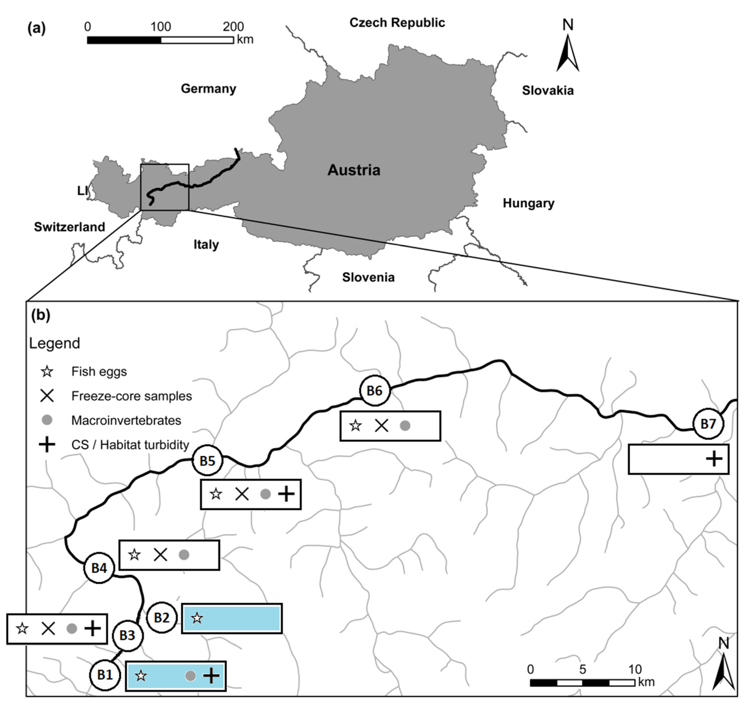
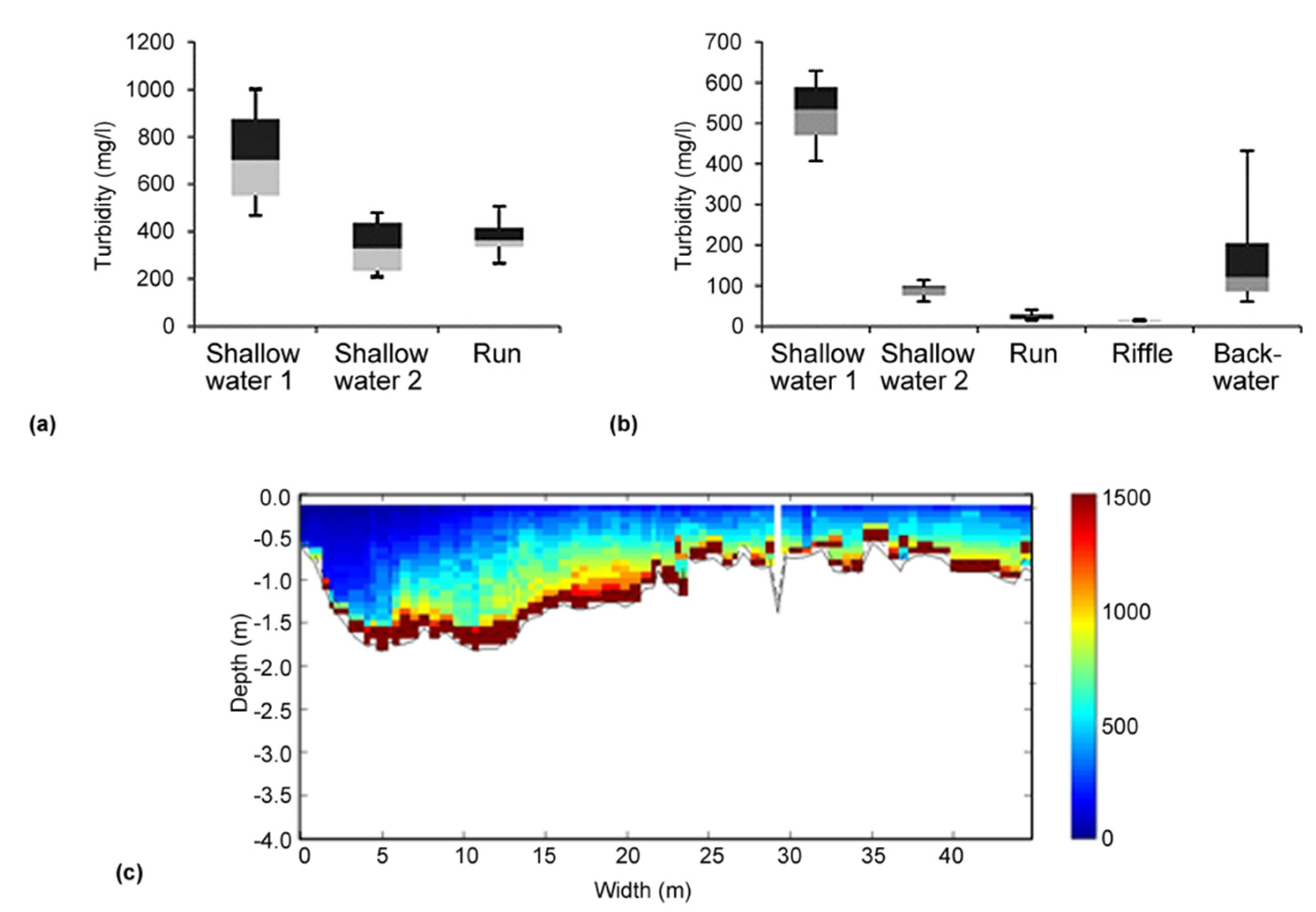
2.1. Cross section Variability and Habitat-Related Turbidity Measurements

The SSC are usually continuously recorded by optical sensors, installed at several sites along the river stretch. However, in most cases the turbidity is only measured at one point (often near the river bank) in the channel cross section, which may be insufficient when no complete mixing is given. To investigate the distribution of fines across the river profile, acoustic backscatter data (ABS) from an ADCP (Acoustic Doppler Current Profiler; Teledyne RDI 300 kHz Workhorse; Teledyne) were used. The ADCP was deployed for measurements at four locations (Ried, Prutz, Imst and Innsbruck; compare Figure 1b) from bridges located at those measurement stations (Figure 1b). To calibrate the ABS data, a point-integrating suspended-sediment sampler (US P-61-A1) was used to derive water samples (and subsequently SSCs) in pre-specified verticals (up to seven verticals and three samples over depth) across the river transects in accordance to available standards; e.g., [32,33,34]. The samples were analyzed with respect to SSC and PSD (particle-size distribution) because the relationship between the ABS, but also the turbidity, measured by turbidity meters, and SSC is strongly dependent on the size, composition and shape of the particles [35].

Furthermore, habitat-related turbidity measurements were examined with a hand-held Solitax ts-line type turbidity sensor from Hach-Lange in discrete hydro-morphological units; c.f. [36,37]. The turbidity was measured in the Prutz area (downstream from the tailrace channel of the HPP Kaunertal, as well as downstream from the mouth of the Fagge river) and in the Karrösten area, where measurements were conducted in different sections of the Inn with hydro-morphological diversity. In each hydro-morphological unit (riffles, run, backwater and shallow water habitats), the turbidity was measured for 1 min at 10 sampling points. In total, n = 30 points were sampled. The time interval for the automatic recording of the measured values was set to 5 s, which resulted in approximately 12 values per measuring point, where a value for the turbidity (NTU) as well as a value for the SSC (mg^−l) were recorded. Based on the data, mean and standard deviation (SD) calculations were performed for (i) shallow water, (ii) run, (iii) riffle and (iv) backwater habitats, according to the classification of Hauer et al. (2009) [37]. Pools and fast runs were excluded due to higher water depths and high flow velocities, respectively.

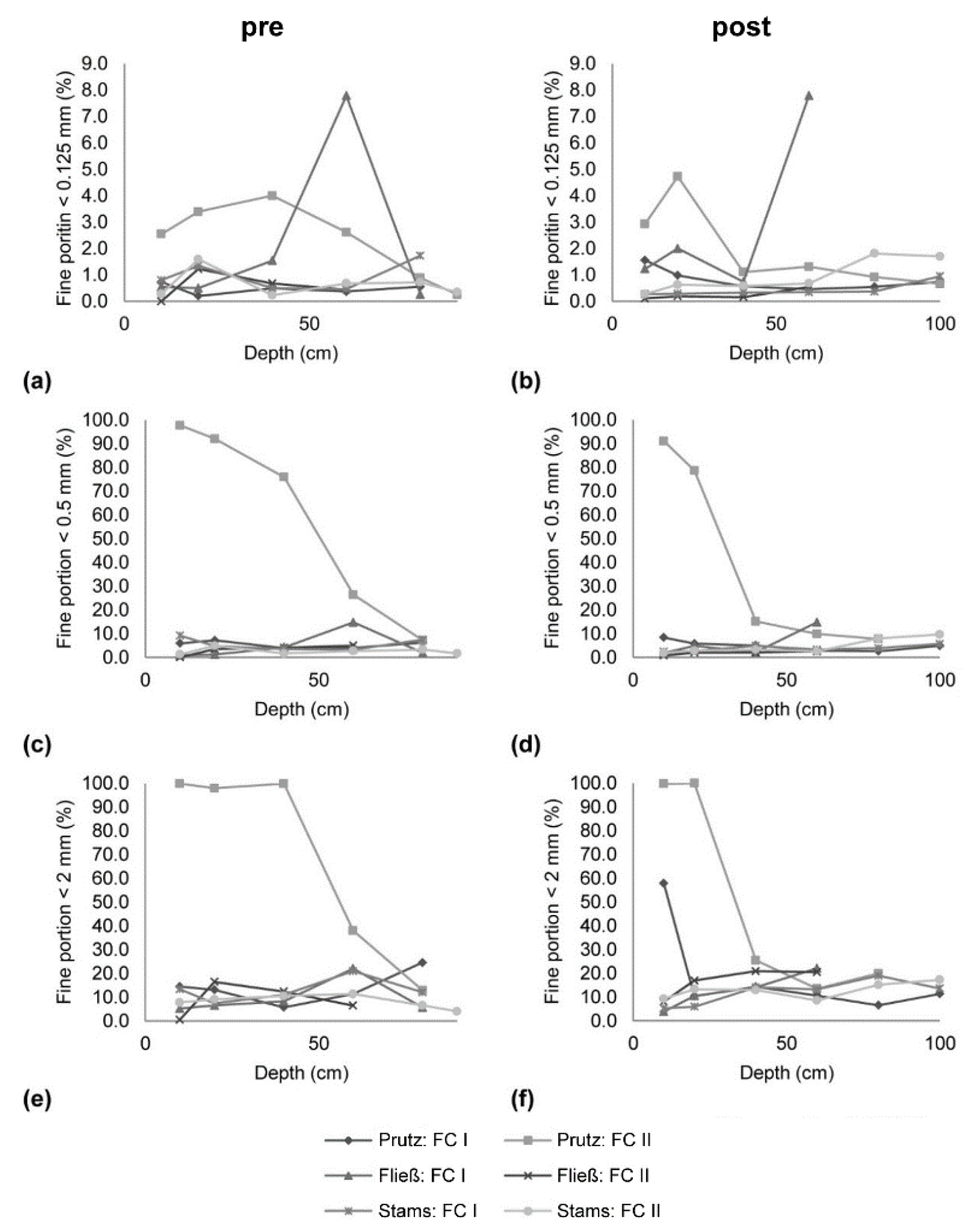
2.2. Freeze-Core Sampling

Sedimentological investigations of the vertical river substrate layers were conducted via freeze-core (FC) sampling [38] in the sections Prutz; Fließ (residual flow stretch); Imst; and in Stams, where a freeze-panel was used instead of a freeze-core (see Figure 1b). For freeze-core sampling, a pointed hollow rod of high-grade steel with a 4.5 cm inner diameter was applied at all sample sites. The rod was driven 0.5 m, 0.75 m or 1 m into the riverbed, depending on the bed material size and silting conditions. Liquid nitrogen (−196 °C) was taken to freeze the surface and the subsurface bed material. An average volume of 40 L per core was applied over a 30 to 45-min freezing period. Depending on the duration of the freezing process, cores with an average diameter of 30 cm were obtained. The stratification of deposited/sorted sediments and the quantification of fines were determined by analyzing the vertical layers with a height of 10 cm and 20 cm, depending on the core length. However, the freeze-cores are spatially limited (average diameter of a sample of 30 cm) and can so only represent a small area [39]. In addition, the results for the coarser fractions tend to be inaccurate due to the limited sampling volume [40], so this approach was taken to quantify possible fine sediment infiltration (FSI) in the gravel matrix due to the increased fine sediment release by the controlled drawdown of the reservoir. Following DIN 4022 (German standard for soil and rock classes), particles in the range between stones/cobbles and clay were analyzed. The samples were dried before sieving was conducted. The following mesh sizes, given in mm, were used: 125, 90, 63, 56, 31.5, 22.4, 16, 11.2, 8, 4, 2, 1, 0.5, 0.25, 0.125, and 0.063. Special attention was given to fines, including the grain sizes of 2.0, 0.5 and 0.125 mm. At each sampling spot, two freeze-cores (FC I & FC II) were taken in minimum to consider the small-scale variability in sediment composition.

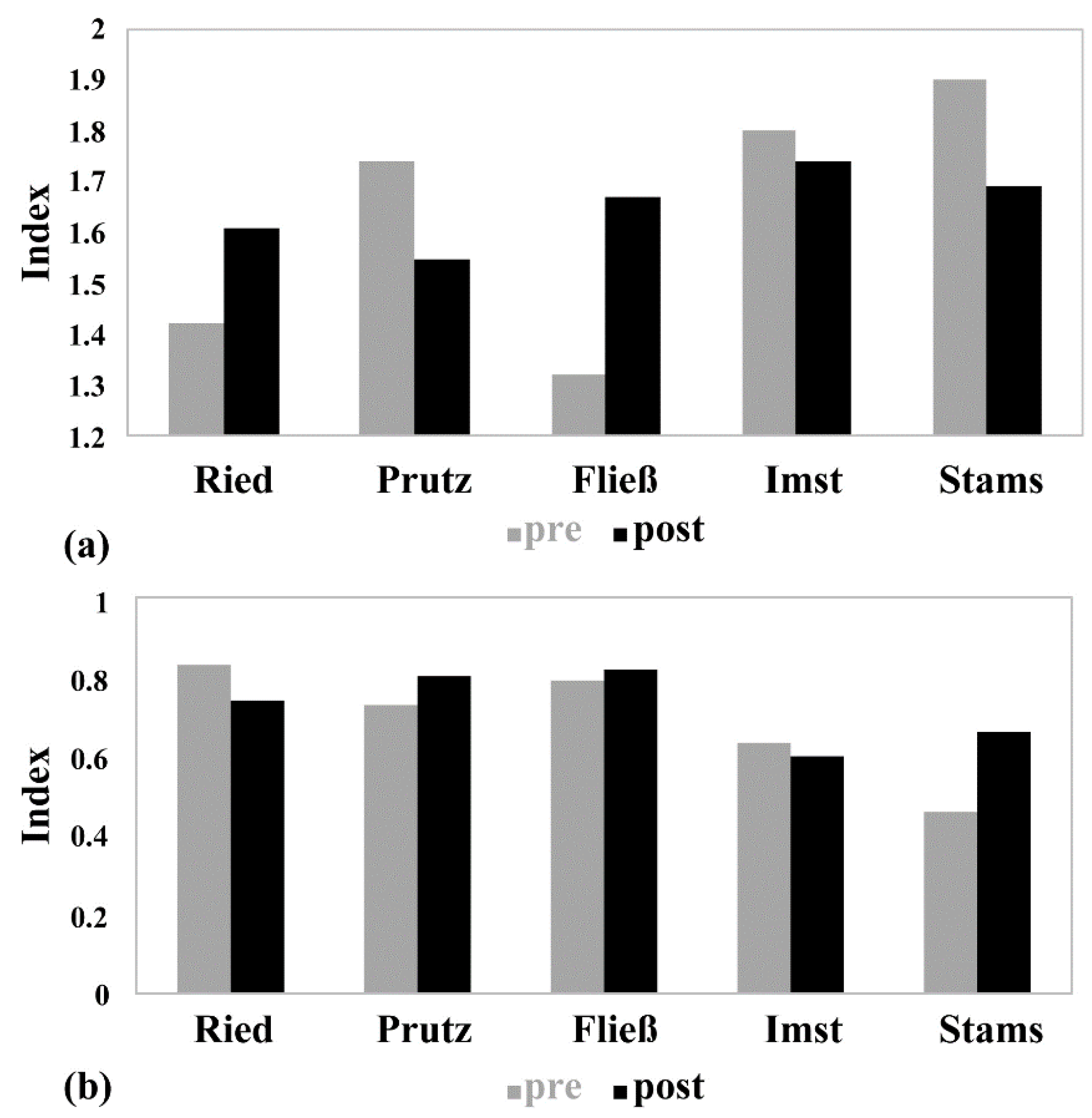
2.3. Macroinvertebrates

For the assessment of macroinvertebrates, a multi-habitat sampling (MHS) approach was used [41]. MHS represents a habitat-weighted evaluation of macroinvertebrates, providing a representative view on the faunal assemblages on minerogenic and organic micro-habitats in a given river stretch. Habitats with less than 5% area coverage were not collected. The samples were taken with a standardized hand net of a 0.25 m frame length and a mesh size of 500 μm. The river bottom was stirred up, corresponding to a projected area of the collecting device (0.25 × 0.25 m), representing a single sample unit.

The 20 sub-samples were not pooled in this study but instead combined according to habitat-specific criteria into compartments of five sample units each. A compartment represents similar hydraulic conditions or grain size distribution. For each single sample, the flow velocity was measured, using a Flo-Mate device (Marsh-McBirney, Model 2000), and the water depths by means of measuring sticks. The sediment type was assessed at each sampling spot by Moog et al. (1999) [42]. At each study site, four different habitat types were distinguished. The summary of all four compartments (equivalent to 20 individual samples, representing an MHS) enables the standardized calculation of the detailed macroinvertebrate method for each position and date according to Ofenböck et al. (2015) [41]. The samples were fixed with formol (4% final concentration) and sent to the laboratory for further processing. All taxa groups of the compartments were sorted, counted and determined to the best possible taxonomic level. The organisms of the single samples, with the exception of the taxonomic group Oligochaeta and the Diptera families Chironomidae and Simuliidae, were also identified to the best possible level and included in a cluster analysis.

The EU Water Framework Directive (WFD, European Commission 2000) proposes a type-specific assessment of the current ecological status by comparing the current situation with a near-natural reference status. The WFD compliant Austrian assessment for macroinvertebrates (detailed macrozoobenthic (MZB) method) is based on two evaluation modules, namely saprobity and general degradation (see guideline according to Ofenböck et al. (2015) [41]). The assessment of the effects of organic pollution (module saprobity) on macroinvertebrates is carried out by applying the saprobic index (SI) according to [42,43,44] based on the respective model-related basic saprobic condition (BSC). The BSC—ranging between 1.0 (minor natural organic load) and 2.0 (high natural organic load)—is required as a typology criterion for the subdivision of bioregions including altitude and catchment size. Thus, the combination of bioregion and BSC defines a river type [41]. According to the Austrian assessment method of the ecological status (European Commission 2000), the investigated water bodies were assigned typologically to a bioregion: AF—Large Alpine Rivers (17), with the inner differentiation Inn, and a BSC of 1.5 for the sites Ried, Prutz and Fließ (residual flow stretch); and a BSC of 1.75 for the sites Imst and Stams, respectively (Figure 1b).

The module “General Degradation” reflects the effects of various stressors (habitat degradation like morphology, damming etc.) and consists of one or two multimetric indices (MMI), depending on the river type. For the present river type only one MMI (MMI1) is foreseen to be calculated. For the overall assessment of a site, the results of both modules are consulted, whereby the ecological status of a sampling site is determined according to a “worst case” approach based on the worst result of both modules. For the calculation of the biological parameters (metrics) by using the detailed MZB method, the data were analyzed with the software ECOPROF, version 4.0 [45]. Although all of the investigated sites were targeted for a good ecological potential (heavily modified water bodies), we assessed the ecological status and interpreted the results in terms of achieving good ecological potential (in accordance to the WFD). The guidelines for achieving a good ecological potential, including the details of the methodology and evaluation, are described in a first approach in [46].

2.4. Fish—Salmonid Incubation

As the controlled drawdown took place in winter during the spawning period of brown trout Salmo trutta f. fario, it was decided to use salmonid eggs as bio-indicators. In this study, fish breeding boxes and sediment boxes in accordance with Holzer et al. (2011) [47] were used. At each of the six selected study sites (Figure 1b), which were all situated on natural spawning places (station 1 (reference site): 100 m upstream of the tailrace of HPP Kaunertal; station 2 (reference site): Fagge tributary to the river Inn/2.54 km upstream of the mouth of the river Fagge; station 3: 2.05 km downstream of the tailrace (emission point); station 4: 8.95 km downstream of the tailrace; station 5: 32.3 km downstream of the tailrace; station 6: 55.16 km downstream of the tailrace), two sediment boxes and one fish breeding box were deployed. Related to the availability of eyed-eggs, the boxes were exposed between 05./06.01.2016 and 05./06.03.2016. The sediment boxes were filled with a sieved 16/32 mm substrate mixture. Due to this procedure, all particle sizes smaller than 16 mm can be assigned to the infiltration during the exposure time. Subsequently, 300 eyed brown trout eggs (Salmo trutta f. fario) were filled in per box. After completion of this work, the boxes were closed and buried in the river substrate. For the evaluation of the variability of the fish breeding box stations, a method for testing a standard distribution (z-test) was used. In the analysis, the actual observed results (obs.oi) of the expectation value [exp. (GV)] of the living and dead larvae were estimated. Afterwards, the procedure of the statistic z-test and Chi²-test was done.

3. Results

3.1. Cross Section Variability and Habitat-Related Turbidity Measurements

The continuous recording of the SSC was based on single point measurements in the selected cross sections and close to the river bank. For aquatic organisms, however, the cross sectional and/or habitat-related variability is of high importance and determines the magnitude of impact. Thus, in Figure 2, selected results at (a) station Fagge mouth (05.02.2016), (b) gravel bar at Prutz (05.02.2016) and (c) the cross-sectional distribution in Prutz are presented.

From Figure 2a, a clear heterogeneity in the distribution of the SSC in the studied river can be seen. Figure 2a exhibits in addition a distinct variability between the various hydromorphological units (shallow water, run, riffle and backwater). Although a clear trend for one specific habitat type with a lower turbidity was not given for all measuring dates (n = 4), it turns out that in all investigated sections of the Inn river, sheltered habitats (in terms of reduced turbidity) were present during the controlled drawdown in winter 2015/2016. Moreover, the ADCP cross sectional measurements (Figure 2c) support the habitat-related turbidity data for deeper parts of the river transects (as accuracy of the ADCP starts at a water depth of 0.5 m). The total cross-sectional variability in the SSC was measured at four stations, namely Ried, Prutz, Haiming, and Innsbruck, where the measurements were conducted a total of three times at each section for different dates (in total four repetitions during the drawdown). Exemplarily shown in Figure 2c are the measurements at Prutz, downstream of the HPP Kaunertal. At the measuring days 21.12.2015 and 04.02.2016, higher concentrations of suspended sediment in the middle and the orographic right half of the profile were observed, while very low concentrations were measured on the left bank. This indicates that at the gauging station Prutz (located approximately 900 m downstream the emission point, which discharges into the Inn river on the right bank), no complete mixing happened. This knowledge was used to set up the monitoring system, and two turbidity sensors were operated during the drawdown on that location—one on the orographic right bank (this value was used for high flows, i.e., >20 m³ s⁻¹) and one on the orographic left bank (this value was used for lower flows, i.e., <20 m³ s⁻¹).

3.2. Freeze-Core Sampling

To determine if a settlement of fines on gravel bars happened, if infiltration into the gravel matrix occurred and if this retention was responsible for the decrease in SSC along the longitudinal profile (compare [15]), local scale freeze-core results were interpreted (Figure 3). Investigating the fine sediments below 0.125 mm, in November 2015 (pre-event phase; Figure 3a), for Prutz FC II, a high share of fine sediments is shown, and for the first sample in Fließ FC I, a higher amount of fines for the depth class of 40–60 cm is shown, representing already a high fine sediment infiltration in some areas. In March 2016 (Figure 3b), the pattern of the grain sizes for the second sampling at Prutz FC II changes, but the distribution of fines is especially close to the surface, which is comparably high. The results for the samples taken at Fließ FC II after the event did not change significantly compared to the samples taken in November 2015 (pre-event). Looking at the analysis for the grain sizes below 0.5 mm, in November 2015 (Figure 3c), the Prutz FC II recorded 100% of sediments < 0.5 mm for the layer closest to the surface. The same can be seen for the near the surface layer in March 2016 (Figure 3d), but for the deeper layers, the portion of fine sediments decreased. Also, for the class of fine sediments below 2 mm (Figure 3e) of the second sample at Prutz FC II, 100% of fine sediment content was observed in the layer closest to the surface. The high percentage of fine sediments in the upper layer was still visible during the observations in March 2016 (Figure 3f), but not for the deeper sections. In this reach, not only sample FC II, but also sample FC I, showed a higher number of fine particles close to the surface. To summarize the results, gained from the freeze-core sampling, at the upstream end at Prutz, the percentage of fine sediments decreased for the second sampling period in March 2016. A hundred percent of the portion of fine sediments of size <0.5 mm as well as <2 mm was close to the surface in November 2015, before the drawdown of the Gepatsch reservoir. In March 2016 (after the drawdown), the number of fines decreased at station Fließ (residual flow stretch), but an increase of fine particles in the depth class of 40–50 cm was recorded. The same was documented for the second measurement campaign (March 2016) at Imst (reach IV) at an FC depth of 60–80 cm below the surface. At the lowermost Stams station, slight coarsening was monitored after the event. It also has to be mentioned that the results may differ between the samples taken before and after (November 2015 and March 2016) for each location, which can be related to regional streams resulting in a different transport capacity.

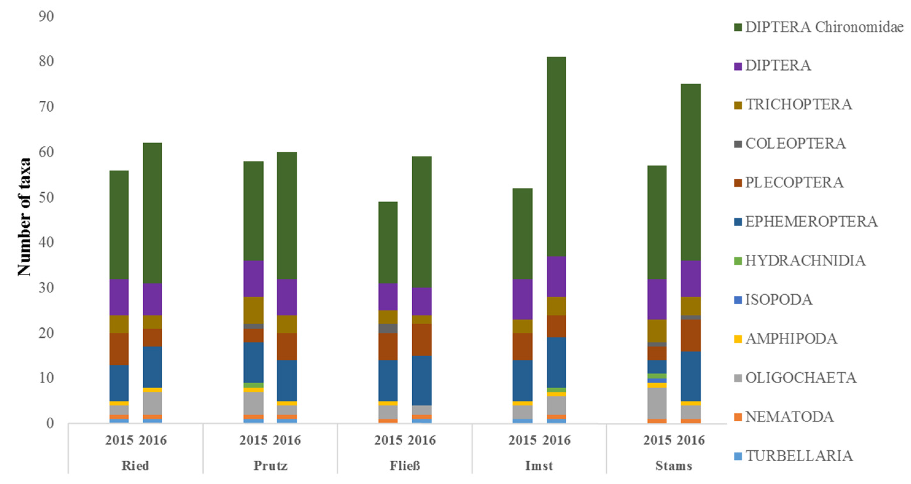
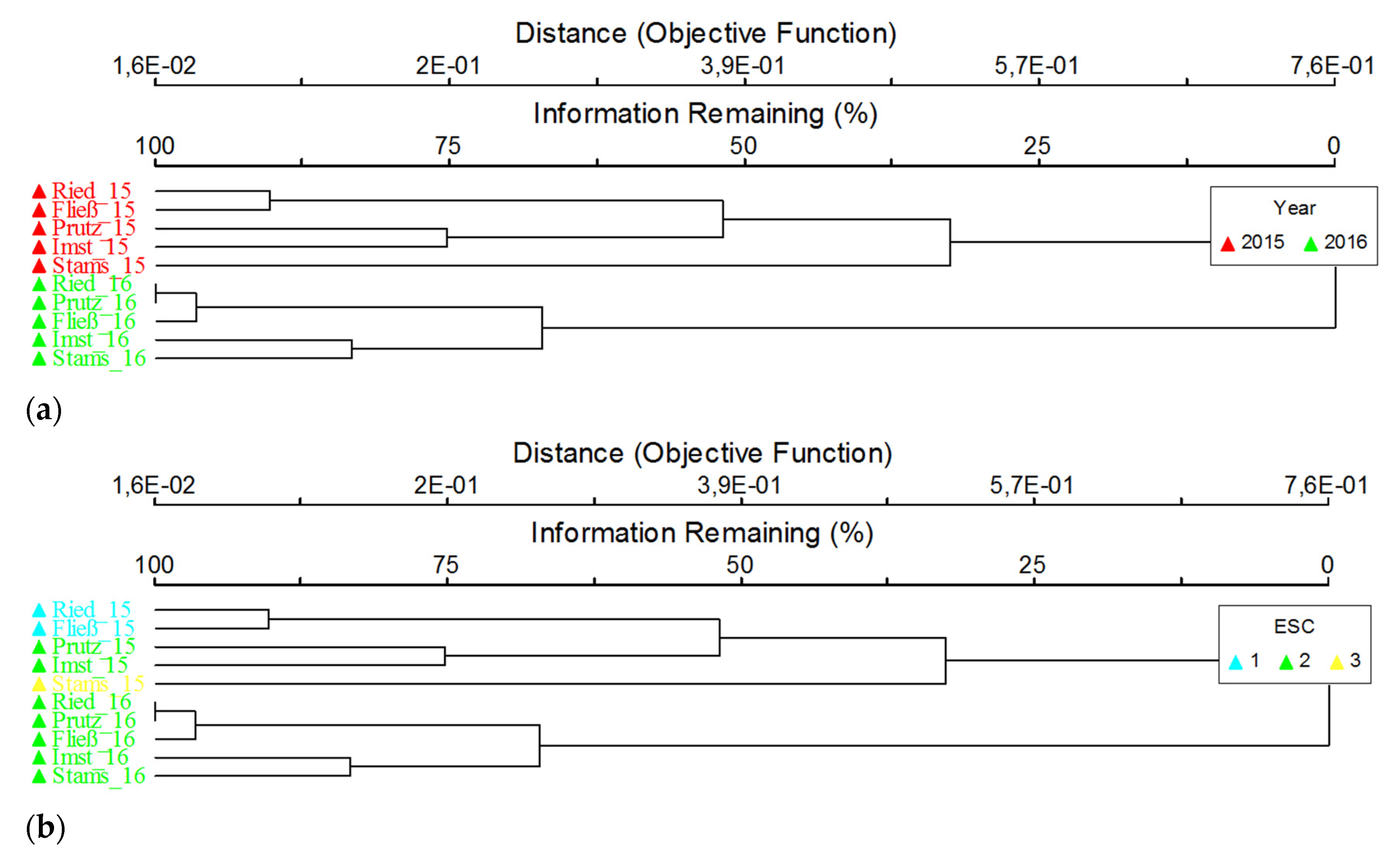
3.3. Macroinvertebrates

The macroinvertebrate community was monitored before and after emptying of the reservoir to detect possible impacts caused by increased fine sediment concentrations. In November 2015, before the measure, the high status (module saprobic index (SI): high; multimetric index 1 (MMI1): high) was indicated at the reference site Ried. At the first investigation site below the power plant initiation, Prutz, a good status (SI: good, MMI1: good), was indicated. In the residual water stretch (Fließ), the SI indicates a high status and the MMI1 a good status (since the index value of the MMI is less than 0.02 points from the next best class boundary, a high ecological status is displayed due to round-up adjustment). Imst and Stams, the last sites in the continuum, indicate good (SI: good, MMI1: good) and moderate (SI: good, MMI1: moderate) ecological statuses, respectively (

Table 1. Ecoprof result of the detailed MZB-method; modules organic pollution (saprobic index, SI), general degradation (multi-metric index, MMI) and the derived ecological status (status).

		Ried	Prutz	Fließ	Imst	Stams
SI	2015	1.42 (high)	1.74 (good)	1.32 (high)	1.8 (good)	1.9 (good)
	2016	1.61 (good)	1.55 (good)	1.67 (good)	1.74 (good)	1.69 (good)
MMI	2015	0.83 (high)	0.73 (good)	0.79 (good)	0.63 (good)	0.46 (moderate)
	2016	0.74 (good)	0.8 (high)	0.82 (high)	0.6 (good)	0.66 (good)
status	2015	high	good	good	good	moderate
	2016	good	good	good	good	good

). The ecological status of the examined water bodies shows clear fluctuations in November 2015, while in March 2016 a uniform status class is indicated.

In March 2016, after the drawdown, a more homogeneous picture emerges, as all study sites indicate a good ecological status (Table 1). Due to the basic saprobic condition (BSC) of 1.75 at the two downstream sites (Imst and Stams), the relatively constant SI indicates a high status. At all other sites with an BSC of 1.5, the SI indicated a good status. With regard to the MMI1, the sites Prutz and Fließ achieve a high status and the remaining sites have good statuses. Figure 4 shows an overview of the modules’ saprobity and general-degradation of both seasons, indicating contrasts. At the Imst investigation site, only marginal differences between the seasons are detectable, where the SI decreases from 1.8 to 1.74, and the MMI1 from 0.63 to 0.6. All other sites show significantly higher seasonal fluctuations for both index values, with the largest change in the SI (deterioration from 1.32 to 1.67) in Fließ, and the highest change in the MMI (improvement from 0.46 to 0.66) in Stams.

In November 2015, the number of MZB taxa shows a range between 49 taxa in the residual flow section (Fließ) and 58 taxa at Prutz (Figure 5). In March 2016, the taxa numbers at all sites were significantly higher, ranging between 59 (Fließ) and 81 (Imst). Having the highest diversity in November 2015, the Prutz site shows the lowest increase (from 58 to 60) in seasonal taxa variation. A general increase in identified taxa numbers in March 2016 is evident, with a significant increase in Chironomidae taxa (Figure 5). All other groups show only minor differences between the sites. The Diptera family Chironomidae provides the highest taxa numbers in all sections, regardless of the sampling date, followed by Ephemeroptera or other Diptera families. Apart from the consistently higher number of Chironomidae taxa, remarkable seasonal differences are detectable at Stams, where the number of Ephemeroptera taxa increased nearly fourfold from three in November 2015 to 11 in March 2016. Additionally, the Plecopteran taxa number increases from three to seven and, in contrast, the number of Oligochaeta taxa decreases from seven to three. Stams is the only stretch where the water hog louse Asellus aquaticus (Isopoda), an indicator for increased organic pollution, was found. Within the sampling campaign in March 2016, however, the taxonomic distribution is similar in all investigated stretches.

Regarding abundance, a significant overall increase between November 2015 and March 2016 is evident, which is mainly explained by the explicit increase of Chironomidae (Figure 5). The lowest numbers of specimens were recorded at both seasons in Prutz, followed by Stams and Ried. In Imst, providing a tripling of the density, the highest increase between the seasons is given. Particularly striking is the high proportion of Oligochaeta specimens in Prutz and Stams in November 2015 and in Imst for both seasons. The benthic communities show major differences between the sites in autumn 2015, resulting in higher differences regarding the modules’ saprobity and general degradation (Figure 4) and the derived ecological status classes (Table 1) compared to the investigation in spring 2016. The consistent longitudinal succession of the coenoses in March 2016 can be confirmed by cluster analyses, according to which the assemblages of the upper sites of Ried, Prutz and Fließ show a high similarity and are well separated from both the lower sites Imst and Stams (Figure 6). This evident separation is not given in November 2015, nevertheless, a clustering of the different status classes (very good, good and moderate) is given.

3.4. Fish: Salmonid Incubation

Another bioindicator regarding the biological effects of increased fine sediment concentrations along the Inn river during the drawdown of the Gepatsch reservoir was considered by the incubation success of brown trout eggs.

Table 2. Summary of the fish breeding box results at the six monitoring stations (n/a: not available).

Measuring Stations with Fish Breeding Boxes	Living Larvae (lL)	Dead Larvae (dL)	Dead Eggs (dE)	Eyed Eggs (eE)	Dissolved Eggs (Difference on 300)	Total Number of Added Eggs	Hatching Rate [(lL) + (dL)]	Survival Rate [(lL) + (eE)]
Station 1	134	38	21	9	98	300	57%	48%
Station 2	254	1	13	13	19	300	85%	85%
Station 3	0	23	234	0	43	300	8%	0%
Station 4	238	11	26	0	25	300	83%	79%
Station 5	n/a	n/a	n/a	n/a	n/a	300	n/a	n/a
Station 6	218	7	24	0	51	300	75%	73%

and

Table 3. Analysis of sediment samples taken from the sediment boxes at the breeding sites.

	Station 1		Station 2		Station 3		Station 4		Station 5 *	Station 6 *
	Box 1	Box 2	Box 1	Box 2	Box 1	Box 2	Box 1	Box 2	Box 1	Box 1
[mm]	{%]	{%]	{%]	{%]	{%]	{%]	{%]	{%]	{%]	{%]
90.00	0.00	0.00	0.00	0.00	0.00	0.00	0.00	0.00	0.00	0.00
63.00	0.00	0.00	0.00	0.00	0.00	0.00	0.00	0.00	0.00	0.00
56.00	0.00	0.00	0.00	0.00	0.00	0.00	0.00	0.00	0.00	0.00
31.50	12.74	16.17	20.87	21.08	21.84	18.86	16.34	15.35	18.93	11.52
22.40	28.31	27.64	29.73	31.82	25.45	23.08	41.60	36.86	27.47	27.02
16.00	29.24	28.09	25.06	26.95	27.56	28.90	23.45	32.44	26.26	31.77
11.20	12.79	7.54	8.80	7.92	7.49	9.15	8.80	7.82	8.53	8.01
8.00	3.18	1.74	1.48	1.19	0.78	1.53	1.73	0.70	1.93	1.42
4.00	3.84	2.48	2.00	0.37	0.15	0.56	0.38	0.19	3.05	2.63
2.00	8.15	13.99	7.99	6.35	5.90	4.55	2.01	1.69	10.21	14.01
1.00
0.50
0.25
0.125	1.76	2.35	4.07	4.33	10.81	13.36	5.69	4.95	3.61	3.62
0.063
pan

Station 1: reference site upstream the tailrace channel; station 2: reference site in the tributary Fagge; station 3: 2.05 km downstream the tailrace channel; station 4: 8.95 km downstream the tailrace channel; station 5: 32.3 km downstream the tailrace channel; station 6: 55.16 km downstream the tailrace channel. * Boxes 2 from station 5 and 6 were lost (no results).

summarize the results of the investigations conducted with the fish breeding boxes at six study sites.

By comparing the survival rate (85%) at examination site 2 (reference, Fagge tributary) in reach Prutz (Inn river at the mouth of the tributary Fagge), a complete failure (0% survival) becomes evident from the data. The reasons for this are the fine sediment load as well as the hydropeaking conditions, which is occurring at the reference site in the Inn river. The other downstream investigation reaches Fließ and Stams, however, it shows good survival rates of 73% and 79%, respectively. Thus, at investigation sites 4 and 6, no negative influence can be detected. At examination site 5, unfortunately, no data is available because the fish breeding box (“cocooning box” [47]) was removed by unknown persons (vandalism). Only an average survival rate (48%) was observed at one reference point, upstream of the tailrace channel of the HPP Kaunertal, which underlines that upstream located stressors (e.g., hydropeaking) already affect the reference site.

The statistical analysis shows that of the five examined sites, with a high set significance factor p < 0.01; the examination sites Fließ and Stams have significantly typical (specifically “many”) living larvae. Investigation site 3 has significantly atypical (specifically “little”) living larvae. The study site Prutz is the only site that does not have significant living larvae. The Chi² [i]-test sharpens the z-test performed and shows at a p of 0.05 that all results except the results of station 1 are significant (df = 4; p = 0.05; value from the Chi² table = 9.488) and not randomly distributed (

Table 4. Test of the uniform distribution of the living and dead larvae of the five investigative spots (z-test, p = 0.01). Green area: significantly typical (specifically “many”) living larvae; red area: significantly atypical (specifically “little”) living larvae; white area: no significance; n/a: not available.

	u [i]	u [i]	χ² [i]	χ² [i]
Fish Breeding Boxes	Living Larvae	Dead Larvae	Living Larvae	Dead Larvae
Station 1	−2.29	2.68	5.27	7.19
Station 2	7.13	−8.33	50.80	69.39
Station 3	−13.16	15.38	173.20	236.58
Station 4	4.92	−5.75	24.24	33.12
Station 5	n/a	n/a	n/a	n/a
Station 6	3.40	−3.98	11.59	15.83
Total			265.10	362.10	χ²
			4	4	df
			0.05	0.05	p

). The values from the Chi² test must be higher than the value from the Chi² table to be statistical significant. Moreover, it was important to document sand fractions and sand infiltration in the various boxes. The highest values are obtained from investigation site 1 (box 2, reference Inn) with 13.9%, investigation site 5 (box 1, Imst) with 10.2%, and investigation site 6 (box 1, Stams) with 14.0%. In all other sediment boxes, the values are below 10% (Table 3).

4. Discussion

In this chapter, the components of the implemented monitoring are grouped and discussed in a more holistic perspective, with a differentiation of the scaling instream processes by means of a local scale. On the local scale, various biotic and abiotic criteria were investigated during monitoring.

According to the survival of brown trout eggs, there are numerous data on the water depths, flow rates, oxygen demand, substrate composition, and critical values of fines in the spawning substrate for the brown trout spawning sites available [48]. Furthermore, a large number of studies deal with fine sediment deposits in brown trout spawning sites < 15 mm [49]. Many of these studies show that the deposition of fine sediments < 2 mm has a major impact on the survival of brown trout eggs. The deposition of fine sediments reduces the permeability/pore space in the spawning substrate, and thus provides less oxygen to the eggs [50,51,52,53,54]. This leads to low survival rates or premature hatching of the larvae [55,56]. Depending on the grain size of the deposited fine sediments, the eggs and larvae react in different ways. Grain sizes < 1 mm or < 2 mm (sand fractions) close to the surface of the spawning site and therefore the hatched larvae have difficulty emerging from the substrate [57]. The data in the literature are scattered here, but sand fractions of 10% to > 20% of the total spawning substrate are considered to be critical. Other studies show that even 1.5% of fines < 0.125 mm (clay and silt fractions) result in severe river bed clogging and are sufficient to severely limit the oxygenation of eggs, and thus, cause high mortalities [58,59]. Comparing the data from the literature with the results from the present study, all values < 2 mm (sand fraction) from the sediment box samples are below the highest critical value of 20% (see Table 3).

A completely different picture is obtained by comparing the critical values of silt and clay fractions (<0.125 mm). In the literature (Louhi et al., 2008), a critical maximum value for fine fractions < 0.125 mm is given to be 1.5%. However, in all sediment boxes, used in this study, the values are above this limit, even significantly in some boxes. The highest values occurred at investigation site 3 (box 1 and box 2) with 10.8% and 13.4%, respectively. At test site Fließ (box 1 and box 2), the fine fractions were approximately 6% and at test site 2 (box 1 and box 2) they were approximately 4%. At all other points, the values ranged between 3.6% and 1.8% (see Table 3). Comparing these values with the hatching rates in the incubators (Table 2), it can be seen that also fine fractions (<0.125 mm) of 3.6% to 5.7% allow high hatching rates (79% residual water in Fließ, 89% reference Fagge and 73% Stams; see Table 2 hatching rates). Thus, it can be clearly seen that the threshold values, which are found in the literature [8], cannot be transferred in a 1:1 approach, and thus, experiments with eyed eggs, and therefore, there is an urgent need for research into fine sediments in spawning grounds.

Self-sustaining fish populations can only become established if all age-stages of the occurring species find suitable habitat conditions. The prevailing habitat forms the basis on which an organism organizes an ecosystem [60]. Consequently, if the habitats of a stream are not suitable for the reproduction of fish, no stable population of this species will be formed. In addition to the quality of the spawning substrate [49,61], inter-gravel flow through the gravel is necessary to carry off metabolic secretions of the incubated eggs; e.g., [62]. To determine the sediment quality for an aquatic organism, freeze-cores have been applied in a number of studies investigating benthic and hyporheic fauna; e.g., [13,15]. The vertical distributions could be described for different river types, habitats and seasons; e.g., [63,64,65]. Even if some criticism has been given to freeze-coring, it is a frequently applied approach for detecting fine sediment infiltration FSI [15], sediment composition in vertical layers [24] and macroinvertebrate habitats. The FC data were taken to compare pre- and post-drawdown sediment composition on the local scale. Even if it was possible to detect some changes in the sediment composition, (e.g., increase of fines for site Fließ), it was not possible to use this information for a clear point of assessment on the local scale, due to the variable and undocumented hydraulic and morphological boundaries. Here, the hydraulic characterization by hydrodynamic-numerical/sediment transport modelling for discrete events (e.g., high-flows for erosion and morphological changes; or cases of high SSC) may be an option to analyze larger scale impacts on the morphodynamics [15]. This was out of the scope of the presented project but should be considered if freeze-cores are part of a monitoring campaign.

The cluster analysis of macroinvertebrates (Figure 6a) clearly revealed a distinct separation of the benthic communities at all sites as a result of the season. Development of eggs and larvae is accelerated for many species during low flow periods in the winter, leading to a natural change in community structure, which hampers a clear cause–effect discussion. Furthermore, at the Inn river, an upper reach (site Ried, upstream of fine sediment release, Prutz and Fließ in March 2016 and sites 1 and 3 in November 2015) and a lower reach (the Imst and Stams sites in March 2016 and Prutz, Imst and Stams in November 2015) can be differentiated (Figure 6a), affirming the classification in saprobic basic conditions of the last two sites. Before the measurements, the sites Prutz (potentially affected by the fine sedimentation as it is located only a few 100 metres downstream of the tailrace channel of the HPP Kaunertal) and Imst were clustered together. Afterwards, the community of the site Prutz was more similar to the reference than to the downstream sites. A more distinctive gap between these two sites should be visible if the Prutz site was really affected by fine sediments.

Overall diversity at each site is higher in March 2016 than in November 2015 (Figure 5), and the total abundance reacts in the same direction (Figure 5). Chironomids are a key player with many species also reproducing during cold periods [66,67], which can strongly influence the benthic community [68]. For example, Gray & Ward (1982) [7] documented a loss of Chironomids up to 90% due to sediment release from a reservoir but reported a recovery to initial levels 3 weeks after the release ended. The saprobic index shows high variation at all sites, except in Imst, and indicates better conditions at three sites in March 2016 than in November 2015 (Figure 4a). The contrary would be expected, as fine sediments are usually poorly oxygenated and tolerant taxa would accumulate; e.g., [69]. The multimetric index deviates mostly at Stams between the seasons and is otherwise similar to November 2015 at the other sites (Figure 4b). Variation in both the diversity and abundance of benthic invertebrates and in the closely linked parameters of the status assessment can hardly be associated with the effect of fine sedimentation after the drawdown of the Gepatsch reservoir. A common trend at Prutz is not visible after the drawdown. Seasonal development of the benthic community seems to be more responsible for this than any external factors. An apparent increased diversity in March 2016 might be an artefact, most likely masked by the occurrence of later larval instars, which simply enable a more exact identification. With some minor exceptions [70,71], comparable long-term baseline information is not available to evaluate seasonal variability at the site spot without the impact of the investigated stressor. In, for example, multiple-stressed river systems [72], local morphological conditions [69] or hydrological events [73] may overrule general settings as, for example, heavy colmation phenomena were recognized during November 2015, which was not the case in March 2016. The reason for this is unknown, as no flood events happened during winter. However, it is possible that the input of (coarse) substrate from the tributaries and sub-catchment scale high flows had a positive effect on the habitat quality during this period, as local sediment quality is decisive for benthic organisms and is able to steer diversity and abundance decisively [74,75,76].

The river Inn in Tyrol is impacted by multiple anthropogenic pressures, such as channelization and hydropeaking. The national assessment system is not designed to identify these specific impacts (e.g., residual flow, pulse-releases), which predominantly affect quantitative aspects of a biocenosis, nor to reveal the effects of multiple stressors [41]. Interestingly, no significant increase in FSI was documented and no significant increase in fine sediment deposits on the gravel bars was detected [15]. However, a clear reduction in SSC was evident in the reach scale perspective. Thus, there is still a lack of process understanding of how tributaries influence the SSC and deposits evolve in the permanent wetted area (e.g., backwater sites downstream of bars or groins).

5. Conclusions

Within this study, local-scale abiotic and biotic elements were evaluated concerning their quality for environmental assessment related to the drawdown of the Gepatsch reservoir. This gained knowledge should on one site improve the process understanding concerning the fine sediment dynamics in an Alpine river and should on the other site recommend monitoring strategies for future projects. It could be documented that not all obtained parameters and methods are of high relevance to support the monitoring questions, such as freeze-core sampling, which exhibited a high local scale variability depending on mid- to long-term hydrological and sedimentological processes in the stretch. In addition, there is a need for an improvement in the biotic evaluation criteria (e.g., inclusion of the parameter biomass for macroinvertebrates) or habitat-specific turbidity measurements. General recommendations: Data on benthic invertebrates between November and March are hardly comparable as seasonal aspects overrule local events. Additionally, different recovery periods for certain invertebrate taxa [7] need to be considered. Long-term baseline information on the “natural” development of the benthic community at the site-scale is essential for identifying natural variability caused by seasonal developments of the benthic community. Additionally, abiotic parameters, such as the discharge, sedimentological turn-over and temperature, have to be registered to interpret the local and reach scale conditions. However, macroinvertebrates are a suitable indicator (e.g., density, diversity, biomass) in such a monitoring programme. Regarding the bioindicator “survival of brown trout eggs” in breeding boxes, the fact that this is dependent on the availability of brown trout eggs (e.g., exposition was on 5 January 2016 in the presented case study) must be considered. In this case study, we used eyed eggs. From another study [77], we know that it is also possible to use green eggs. However, due to the time constraint (availability of green and/or eyed eggs), this method is barely applicable to monitoring projects. In contrast, other local scale parameters were supportive, such as the habitat and cross-sectional variability in SSC.

In summary, based on the integrative monitoring of the controlled drawdown of the Gepatsch reservoir in winter 2015/16 (compare also to part A), it can be concluded that (i) no overtopping of thresholds of the permit was documented and a clear reduction in SSC could be detected along the course of the river Inn; compare to [15]. Moreover, (ii) there were no fine sediment deposits or changes in the fine sediment deposits on the gravel bars, which means that a controlled drawdown in winter may contain beneficial aspects, since no overtopping of gravel bars occurs due to the low base flow. Our study [15] (and this publication), revealed insight into an integrative and innovative monitoring concept (abiotic and biotic parameters) during the controlled release of water from the Gepatsch reservoir. In this context it was also important to analyze technical aspects, i.e. turbine abrasion [78]. So far, a few studies have considered integrative monitoring and management for reservoir flushing [79], while data for a controlled reservoir drawdown was scattered. Thus our case study forms a basis for a sustainable reservoir management of Alpine reservoirs in the future.

References

1. Zarfl, C.; Lumsdon, A.E.; Berlekamp, J.; Tydecks, L.; Tockner, K. A global boom in hydropower dam construction. Aquat. Sci. 2015, 77, 161–170. [Google Scholar] [CrossRef]
2. Moog, O. Quantification of daily peak hydropower effects on aquatic fauna and management to minimize environmental impacts. Regul. Rivers Res. Manag. 1993, 8, 5–14. [Google Scholar] [CrossRef]
3. Hauer, C.; Holzapfel, P.; Leitner, P.; Graf, W. Longitudinal assessment of hydropeaking impacts on various scales for an improved process understanding and the design of mitigation measures. Sci. Total Environ. 2017, 575, 1503–1514. [Google Scholar] [CrossRef]
4. Dugan, P.J.; Barlow, C.; Agostinho, A.A.; Baran, E.; Cada, G.F.; Chen, D.; Marmulla, G. Fish migration, dams, and loss of ecosystem services in the Mekong basin. AMBIO 2010, 39, 344–348. [Google Scholar] [CrossRef] [PubMed] [Green Version]
5. Anderson, E.P.; Freeman, M.C.; Pringle, C.M. Ecological consequences of hydropower development in Central America: Impacts of small dams and water diversion on neotropical stream fish assemblages. River Res. Appl. 2006, 22, 397–411. [Google Scholar] [CrossRef]
6. Ziv, G.; Baran, E.; Nam, S.; Rodríguez-Iturbe, I.; Levin, S.A. Trading-off fish biodiversity, food security, and hydropower in the Mekong River Basin. Proc. Natl. Acad. Sci. USA 2012, 109, 5609–5614. [Google Scholar] [CrossRef] [Green Version]
7. Gray, L.J.; Ward, J.V. Effects of sediment releases from a reservoir on stream macroinvertebrates. Hydrobiologia 1982, 96, 177–184. [Google Scholar] [CrossRef]
8. Kemp, P.; Sear, D.; Collins, A.; Naden, P.; Jones, I. The impacts of fine sediment on riverine fish. Hydrol. Process. 2011, 25, 1800–1821. [Google Scholar] [CrossRef]
9. Crosa, G.; Castelli, E.; Gentili, G.; Espa, P. Effects of suspended sediments from reservoir flushing on fish and macroinvertebrates in an alpine stream. Aquat. Sci. 2010, 72, 85–95. [Google Scholar] [CrossRef]
10. Hauer, C.; Holzapfel, P.; Tonolla, D.; Habersack, H.; Zolezzi, G. In situ measurements of fine sediment infiltration (FSI) in gravel-bed rivers with a hydropeaking flow regime. Earth Surf. Process. Landf. 2019, 44, 433–448. [Google Scholar] [CrossRef] [Green Version]
11. Smith, E.P.; Orvos, B.W.; Cairns, J.J. Impact assessment using the Before-After-Control-Impact (BACI) model: Concerns and comments. Can. J. Fish. Aquat. Sci. 1993, 50, 627–637. [Google Scholar] [CrossRef]
12. Smokorowski, K.E.; Bradford, M.J.; Clarke, K.D.; Clément, M.; Gregory, R.S.; Randall, R.G. Assessing the Effectiveness of Habitat Offset Activities in Canada: Monitoring Design and Metrics; Canada, 2015. Available online: https://waves-vagues.dfo-mpo.gc.ca/Library/347555.pdf (accessed on 1 March 2020).
13. Seitz, L.; Noack, M.; Haun, S.; Reindl, R.; Senn, G.; Schletterer, M. Analysing sediment characteristics of the alpine river Brixentaler Ache (Austria) including in situ measurements of dissolved oxygen. In Proceedings of the 13th International Symposium on River Sedimentation, Stuttgart, Germany, 19–22 September 2016; pp. 915–921. [Google Scholar]
14. Evans, E.; Wilcox, A.C. Fine sediment infiltration dynamics in a gravel-bed river following a sediment pulse. River Res. Appl. 2014, 30, 372–384. [Google Scholar] [CrossRef]
15. Hauer, C.; Holzapfel, P.; Flödl, P.; Wagner, B.; Graf, W.; Leitner, P.; Holzer, G.; Haun, S.; Hammer, A.; Habersack, H.; et al. Controlled reservoir drawdown-challenges for sediment management and integrative monitoring: An Austrian case study—Part A: Reach Scale. Water 2020. [Google Scholar]
16. McLeay, D.J.; Birtwell, I.K.; Hartman, G.H.; Ennis, G.L. Response of Arctic Grayling (Thymallusarcticus) to acute and prolonged exposure to Yukon placer mining sediment. Can. J. Fish. Aquat. Sci. 1987, 44, 658–673. [Google Scholar] [CrossRef]
17. Doeg, T.J.; Milledge, G.A. Effect of experimentally increasing concentration of suspended sediment on macroinvertebrate drift. Mar. Freshw. Res. 1991, 42, 519–526. [Google Scholar] [CrossRef]
18. Newcombe, C.P.; MacDonald, D.D. Effects of suspended sediments on aquatic ecosystems. North Am. J. Fish. Manag. 1991, 11, 72–82. [Google Scholar] [CrossRef]
19. Auld, A.H.; Schubel, J.R. Effects of suspended sediment on fish eggs and larvae: A laboratory assessment. Estuar. Coast. Mar. Sci. 1978, 6, 153–164. [Google Scholar] [CrossRef]
20. Newcombe, C.P.; Jensen, J.O. Channel suspended sediment and fisheries: A synthesis for quantitative assessment of risk and impact. North Am. J. Fish. Manag. 1996, 16, 693–727. [Google Scholar] [CrossRef]
21. Walkotten, W.J. A Freezing Technique for Sampling Streambed Gravel; Northwest Forest and Range Experimental Station: Portland, OR, USA, 1976. [Google Scholar]
22. Carling, P.A.; Reader, N.A. A freeze-sampling technique suitable for coarse river bed-material. Sediment. Geol. 1981, 29, 233–239. [Google Scholar] [CrossRef]
23. Kondolf, G.M.; Lisle, T.E. Measuring bed sediment. In Tools in Fluvial Geomorphology; Kondolf, G.M., Piégay, H., Eds.; Wiley Blackwell: Hoboken, NJ, USA, 2016; pp. 278–305. [Google Scholar]
24. Bunte, K.; Abt, S.R. Sampling Surface and Subsurface Particle-Size Distributions in Wadable Gravel- and Cobble-Bed Streams for Analyses in Sediment. Transport, Hydraulics and Streambed Monitoring; USDA: Washington, DC, USA, 2001.
25. Tritthart, M.; Haimann, M.; Habersack, H.; Hauer, C. Spatio-temporal variability of suspended sediments in rivers and ecological implications of reservoir flushing operations. River Res. Appl. 2019, 35, 918–931. [Google Scholar] [CrossRef] [Green Version]
26. Baran, E.; Nasielski, J. Reservoir Sediment Flushing and Fish Resources; Natural Heritage Institute: San Francisco, CA, USA, 2011. [Google Scholar]
27. Scheurer, T.; Molinari, P. Experimental floods in the River Spöl, Swiss National Park: Framework, objectives and design. Aquat. Sci. 2003, 65, 183–190. [Google Scholar] [CrossRef]
28. Wendelaar Bonga, S.E. The stress response in fish. Physiol. Rev. 1997, 77, 591–625. [Google Scholar] [CrossRef]
29. Gorman, O.; Karr, J.R. Habitat Structure and Stream Fish Communities. Ecology 1978, 59, 507–515. [Google Scholar] [CrossRef]
30. Glova, G.J.; McInerney, J.E. Critical swimming speeds of coho salmon (Oncorhynchus kisutch) fry to smolt stages in relation to salinity and temperature. J. Fish. Board Can. 1977, 34, 151–154. [Google Scholar] [CrossRef]
31. Schletterer, M.; Hofer, B.; Obendorfer, R.; Hammer, A.; Hubmann, M.; Schwarzenberger, R.; Boschi, M.; Haun, S.; Haimann, M.; Holzapfel, P.; et al. Integrative monitoring approaches for the sediment management in Alpine reservoirs: Case study Gepatsch (HPP Kaunertal, Tyrol). In Proceedings of the 13th International Symposium on River Sedimentation, Stuttgart, Germany, 19–22 September 2016; pp. 1161–1169. [Google Scholar]
32. Edwards, T.K.; Glysson, G.D. Field Methods for Measurement of Fluvial Sediment; U.S. Geological Survey, Techniques of Water-Resources Investigations, 1999. Available online: https://pubs.usgs.gov/twri/twri3-c2/ (accessed on 18 March 2020).
33. Haun, S.; Rüther, N.; Baranya, S.; Guerrero, M. Comparison of real time suspended sediment transport measurements in river environment by LISST instruments in stationary and moving operation mode. Flow Meas. Instrum. 2015, 41, 10–17. [Google Scholar] [CrossRef]
34. Haun, S.; Lizano, L. Sensitivity analysis of sediment flux derived by laser diffraction and acoustic backscatter within a reservoir. Int. J. Sediment. Res. 2018, 33, 18–26. [Google Scholar] [CrossRef]
35. Christopher James, G. Potential of turbidity monitoring for measuring the transport of suspended solids in streams. Hydrol. Process. 1995, 9, 83–97. [Google Scholar]
36. Hauer, C.; Unfer, G.; Tritthart, M.; Formann, E.; Habersack, H. Variability of mesohabitat characteristics in riffle-pool reaches: Testing an integrative evaluation concept (FGC) for MEM-application. River Res. Appl. 2011, 27, 403–430. [Google Scholar] [CrossRef]
37. Hauer, C.; Mandlburger, G.; Habersack, H. Hydraulically related hydro-morphological units: Description based on a new conceptual mesohabitat evaluation model (MEM) using LiDAR data as geometric input. River Res. Appl. 2009, 25, 29–47. [Google Scholar] [CrossRef]
38. Humpesch, U.H.; Niederreiter, R. Freeze-core method for sampling the vertical distribution of the macrozoobenthos in the main channel of a large deep river, the River Danube at kilometre 1889. Large Rivers 1993, 9, 87–90. [Google Scholar] [CrossRef]
39. Lisle, T.E.; Eads, R.E. Methods to Measure Sedimentation of Spawning Gravels; Pacific Southwest Research Station, Forest Service, US Department of Agriculture: Berkeley, CA, USA, 1991.
40. Zimmermann, A.E.; Lapointe, M. Intergranular flow velocity through salmonid redds: Sensitivity to fines infiltration from low intensity sediment transport events. River Res. Appl. 2005, 21, 865–881. [Google Scholar] [CrossRef]
41. Ofenböck, T.; Moog, O.; Hartmann, A.; Stubauer, I. Leitfaden zur Erhebung der Biologischen Qualitätselemente, Teil A2—Makrozoobenthos; Umwelt und Wasserwirtschaft: Vienna, Austria, 2015; Available online: https://www.bmlrt.gv.at/wasser/wisa/fachinformation/ngp/ngp-2009/hintergrunddokumente/methodik/biologische_qe.html (accessed on 13 November 2019).
42. Moog, D.B.; Whiting, P.J.; Thomas, R.B. Streamflow record extension using power transformations and application to sediment transport. Water Resour. Res. 1999, 35, 243–254. [Google Scholar] [CrossRef]
43. Wien, Ö.N. ÖNORM M 6232—Richtlinie für die ökologische Untersuchung und Bewertung von Fließgewässern. 1997, p. 38. Available online: https://shop.austrian-standards.at/action/de/public/details/54417/OENORM_M_6232_1997_05_01 (accessed on 13 November 2019).
44. Zelinka, M.; Marvan, P. Zur Präzisierung der biologischen Klassifikation der Reinheit fließender Gewässer. Arch. Hydrobiol. 1961, 57, 389–407. [Google Scholar]
45. Moog, O.; Hartmann, A.; Schmidt-Kloiber, A.; Vogl, R.; Koller-Kreimel, V. ECOPROF—Version 4.0. Software zur Bewertung des Ökologischen Zustandes von Fliessgewässern nach WRRL. 2013. Available online: https://www.ecoprof.at/ (accessed on 13 November 2019).
46. Eberstaller, J.; Köck, J.; Haunschmid, R.; Jagsch, A.; Ratschan, C.; Zauner, G. Leitfanden zur Bewertung Erheblich Veränderter Gewässer—Biologische Definition des Guten Ökologischen Potentials; IA des Bundesministeriums für Land-und Forstwirtschaft, Umwelt und Wasserwirtschaft: Vienna, Austria, 2015; Available online: https://www.bmlrt.gv.at/wasser/wasser-oesterreich/plan_gewaesser_ngp/nationaler_gewaesserbewirtschaftungsplan-ngp/hmwb_lf.html (accessed on 13 November 2019).
47. Holzer, G.; Unfer, G.; Hinterhofer, M. Cocooning—eine alternative Methode zur fischereilichen Bewirtschaftung. Österreichs Fischerei 2011, 64, 16–27. [Google Scholar]
48. Louhi, P.A.; Mäki-Petä, Y.S.; Erkinaro, J. Spawning habitat of Atlantic salmon and Brown trout: General criteria and intragravel factors. River Res. Appl. 2008, 24, 330–339. [Google Scholar] [CrossRef]
49. Pulg, U.; Barlaup, B.T.; Sternecker, K.; Trepl, L.; Unfer, G. Restoration of spawning habitats of brown trout (Salmo trutta) in a regulated chalk stream. River Res. Appl. 2013, 29, 172–182. [Google Scholar] [CrossRef]
50. Chapman, D.W. Critical review of variables used to define effects of fines in redds of large salmonids. Trans. Am. Fish. Soc. 1988, 117, 1–21. [Google Scholar] [CrossRef]
51. Lisle, T.E. Sediment transport and resulting deposition in spawning gravels, North coastal California. Water Resour. Res. 1989, 25, 1303–1319. [Google Scholar] [CrossRef] [Green Version]
52. Pauwels, S.J.; Haines, T.A. Survival, hatching, and emergence success of Atlantic salmon eggs planted in three Maine streams. North Am. J. Fish. Manag. 1994, 14, 125–130. [Google Scholar] [CrossRef] [Green Version]
53. Sear, D.A. Fine sediment infiltration into gravel spawning beds within a regulated river experiencing floods: Ecological implications for salmonids. Regul. Rivers Res. Manag. 1993, 8, 373–390. [Google Scholar] [CrossRef]
54. Seitz, L.; Christian, H.; Noack, M.; Wieprecht, S. From picture to porosity of river bed material using Structure-from-Motion with Multi-View-Stereo. Geomorphology 2018, 306, 80–89. [Google Scholar] [CrossRef]
55. Tappel, P.D.; Bjornn, T.C. A new method of relating size of spawning gravel to salmonid embryo survival. North Am. J. Fish. Manag. 1983, 3, 123–135. [Google Scholar] [CrossRef] [Green Version]
56. Olsson, T.I.; Näslund, I. Effects of mire drainage and peat extraction on benthic invertebrates and fish. In Proceedings of the International Peat Society Symposium; IPS: Hasselfors, Sweden, 1985; pp. 147–152. [Google Scholar]
57. Kondolf, G.M. Assessing salmonid spawning gravel quality. Trans. Am. Fish. Soc. 2000, 129, 262–281. [Google Scholar] [CrossRef]
58. Lapointe, M.F.; Bergeron, N.E.; Berube, F.; Pouliot, M.A.; Johnston, P. Interactive effects of substrate sand and silt contents, redd-scale hydraulic gradients, and interstitial velocities on egg-to-emergence survival of Atlantic salmon (Salmo salar). Can. J. Fish. Aquat. Sci. 2004, 61, 2271–2277. [Google Scholar] [CrossRef] [Green Version]
59. Greig, S.M.; Sear, D.A.; Smallman, D.; Carling, P.A. Impact of clay particles on the cutaneous exchange of oxygen across the chorion of Atlantic salmon eggs. J. Fish. Biol. 2005, 66, 1681–1691. [Google Scholar] [CrossRef]
60. Schoener, T.W. Resource partitioning in ecological communities. Science 1974, 185, 27–39. [Google Scholar] [CrossRef] [PubMed]
61. Hauer, C.; Unfer, G.; Holzapfel, P.; Haimann, M.; Habersack, H. Impact of channel bar form and grain size variability on estimated stranding risk of juvenile brown trout during hydropeaking. Earth Surf. Process. Landf. 2014, 39, 1622–1641. [Google Scholar] [CrossRef]
62. Kondolf, G.M.; Williams, J.G.; Horner, T.C.; Milan, D. Assessing physical quality of spawning habitat. In Salmonid Spawning Habitat in Rivers; Sear, D.A., DeVries, P., Eds.; The American Fisheries Society, American Fisheries Society Symposium: Bethesda, MD, USA, 2008; p. 65. [Google Scholar]
63. Adkins, S.C.; Winterbourn, M.J. Vertical distribution and abundance of invertebrates in two New Zealand stream beds: A freeze coring study. Hydrobiologia 1999, 400, 55–62. [Google Scholar] [CrossRef]
64. Newbold, J.D.; Thomas, S.A.; Minshall, G.W.; Cushing, C.E.; Georgian, T. Deposition, benthic residence, and resuspension of fine organic particles in a mountain stream. Limnol. Oceanogr. 2005, 50, 1571–1580. [Google Scholar] [CrossRef]
65. Weigelhofer, G.; Waringer, J. Vertical distribution of benthic macroinvertebrates in riffles versus deep runs with differing contents of fine sediments (Weidlingbach, Austria). Int. Rev. Hydrobiol. 2003, 88, 304–313. [Google Scholar] [CrossRef]
66. Soszynska-Maj, A.; Paasivirta, L.; Giłka, W. Why on the snow? Winter emergence strategies of snow-active Chironomidae (Diptera) in Poland. Insect Sci. 2016, 23, 754–770. [Google Scholar] [CrossRef] [PubMed]
67. Anderson, A.M.; Ferrington, L.C. Resistance and resilience of winter-emerging Chironomidae (Diptera) to a flood event: Implications for Minnesota trout streams. Hydrobiologia 2013, 707, 59–71. [Google Scholar] [CrossRef]
68. Armitage, P.D.; Blackburn, J.H. Environmental stability and communities of Chironomidae (Diptera) in a regulated river. River Res. Appl. 1990, 5, 319–328. [Google Scholar] [CrossRef]
69. Wood, P.J.; Armitage, P.D. Biological effects of fine sediment in the lotic environment. Environ. Manag. 1997, 21, 203–217. [Google Scholar] [CrossRef] [PubMed]
70. Robinson, C.T.; Uehlinger, U.; Monaghan, M.T. Stream ecosystem response to multiple experimental floods from a reservoir. River Res. Appl. 2004, 20, 359–377. [Google Scholar] [CrossRef]
71. Robinson, C.T.; Uehlinger, U.; Monaghan, M.T. Effects of a multi-year experimental flood regime on macroinvertebrates downstream of a reservoir. Aquat. Sci. 2003, 65, 210–222. [Google Scholar] [CrossRef] [Green Version]
72. Hering, D.; Carvalho, L.; Argillier, C.; Beklioglu, M.; Borja, A.; Cardoso, A.C.; Duel, H.; Ferreira, T.; Globevnik, L.; Hanganu, J.; et al. Managing aquatic ecosystems and water resources under multiple stress—An introduction to the MARS project. Sci. Total Environ. 2015, 503–504, 10–21. [Google Scholar] [CrossRef] [PubMed]
73. Statzner, B.; Higler, B. Stream Hydraulics as a Major Determinant of Benthic Invertebrate Zonation Patterns. Freshw. Biol. 1986, 16, 127–139. [Google Scholar] [CrossRef]
74. Hynes, H.B.N. The Effects of Sediment on the Biota in Running water in Fluvial Processes and Sedimentation. In Proceedings of the Hydrology Symposium; National Research Council: Edmonton, AB, Canada, 1973; pp. 151–169. [Google Scholar]
75. Richards, C.; Bacon, K.L. Influence of fine sediment on macroinvertebrate colonisation of surface and hyporheic stream sediments. Great Basin Nat. 1994, 54, 106–113. [Google Scholar]
76. Descloux, S.; Datry, T.; Marmonier, P. Benthic and hyporheic invertebrate assemblages along a gradient of increasing streambed colmation by fine sediment. Aquat. Sci. 2013, 75, 493–507. [Google Scholar] [CrossRef]
77. Holzer, G. Projekt Ilz: Teilprojekt Brutboxen (Cocooning) 2016. Available online: https://www.researchgate.net/publication/275016473_Cocooning_-_eine_alternative_Methode_zur_fischereilichen_Bewirtschaftung (accessed on 8 April 2020).
78. Fernandes, J.N.; Boes, R.M.; Titzschkau, M.; Hammer, A.; Haun, S.; Schletterer, M. Sediment load, hydro-abrasive erosion and efficiency changes at high-head turbines during the drawdown of two Alpine reservoirs via the power waterway. In Proceedings of the HYDRO 2016—Hydropower and Dams, International Conference and Exhibition, Montreux, Switzerland, 10–12 October 2016. [Google Scholar]
79. Espa, P.; Brignoli, M.L.; Crosa, G.; Gentili, G.; Quadroni, S. Controlled sediment flushing at the Cancano Reservoir (Italian Alps): Management of the operation and downstream environmental impact. J. Environ. Manag. 2016, 182, 1–12. [Google Scholar] [CrossRef] [PubMed]
Figure 1. (a) Map of Austria with the sampled Inn river highlighted; (b) detailed map of the Inn river with highlighted investigations of macroinvertebrates and egg incubation, freeze-core samples and cross-sectional variability, and habitat-related turbidity; blue = reference sites at the Inn (B1) and the tributary Fagge (B2)
Water 12 01055 g001
Figure 2. (a + b) Habitat-related variation in turbidity at two different sites and different dates during the controlled drawdown of the Gepatsch reservoir; measuring time at each habitat type: 10 min; box plots: different grey shadings represent 50% of the analyzed data; (c) Cross sectional plot of the ADCP-recorded turbidity (SSC in mg L−1) at Prutz (04.02.2016).
Water 12 01055 g002
Figure 3. Comparison of fine sediment infiltration in the gravel matrix for the pre- and post-monitoring period; fines < 0.125 mm (a) pre- and (b) post-; fines < 0.250 mm (c) pre- and (d) post-; fines < 2 mm (e) pre- and (f) post-monitoring; reach 1 = Prutz, reach 2 = Fließ, reach 4 = Imst (compare to Figure 1).
Water 12 01055 g003
Figure 4. (a) Saprobic Index and (b) multimetric index in the longitudinal river course of both seasons (November 2015 vs. March 2016).
Water 12 01055 g004
Figure 5. Taxa numbers per taxa group at each site and sampling date (November 2015 vs. March 2016).
Water 12 01055 g005
Figure 6. Cluster analyses; dendrogram; all sites (annex to site labels: 15 = 2015, 16 = 2016), both sampling dates; overlays; (a) sampling date (year: 2015 = November 2015, 2016 = March 2016); (b) ecological status class (ESC; status; 1 = high, 2 = good, 3 = moderate).
Water 12 01055 g006