Are Frontier Efficiency Methods Adequate to Compare the Efficiency of Water Utilities for Regulatory Purposes?
by
 ,
,
Elvira Estruch-Juan
1,* ,
,
Enrique Cabrera, Jr.
1,
María Molinos-Senante
2 and 
Alexandros Maziotis
3 1
ITA, Universitat Politècnica de València, 46020 València, Spain
2
Centro de Desarrollo Urbano Sustentable, Santiago 15110020, Chile
3
Foundazione Eni Enrico Mattei, 30135 Venice, Italy
*
Author to whom correspondence should be addressed.
Water 2020, 12(4), 1046; https://doi.org/10.3390/w12041046
Submission received: 5 January 2020
/
Revised: 1 April 2020
/
Accepted: 2 April 2020
/
Published: 7 April 2020
(This article belongs to the Special Issue Management of Urban Water Services)
Abstract
:Frontier efficiency methods have been recurrently used in the water sector to assess the performance of water utilities. These methods are also used for yardstick regulation, with greater efficiency being sought by creating competition between the utilities, which can have an impact on decision-making processes, such as tariff setting. This study analyzes the adequacy and limitations of these methods for regulatory purposes, particularly how they deal with data uncertainty and their capacity to manage large number of variables. In order to achieve this, two representative methods—a nonparametric technique (data envelopment analysis) and an econometric one (stochastic frontier analysis)—are applied to an audited sample of 194 water utilities. Results will show that the results from the methods may not be considered conclusive in the water sector and their application should be carried out with considerable reservations.
1. Introduction
Urban water services are natural monopolies because regardless of the number of companies providing the service, the demand can be covered at a lower cost by only one company [1].
Due to the monopolistic nature of the water sector, utilities have little incentive to improve the quality of service or their efficiency, unless a regulatory framework encourages it. Yardstick regulation appeared as a tool to incentivize the competition among utilities in a monopolistic market. For that purpose, the performance of the different utilities is compared, creating an artificial competitive market, in order to promote efficiency [2].
The rationale for yardstick regulation is clear in the case of identical utilities. The ones with the worst performance must become more inefficient. However, the presents a challenge when comparing utilities with different exogenous characteristics that affect performance, as is the case in the water sector. In order to overcome this drawback, Shleifer [2] suggested first listing the characteristics by which the utilities differ. Then, regression techniques can be used to perform the comparison, considering these exogenous characteristics.
According to Coelli and Walding [3] and CEPAL (United Nations Economic Commission for Latin America and the Caribbean, CEPAL stands for its acronym in Spanish) [4], there are four main families of methods used to assess the efficiency of a utility:
- Partial efficiency measures;
- Average efficiency measures;
- Econometric frontier efficiency methods;
- Non-parametric frontier efficiency methods.
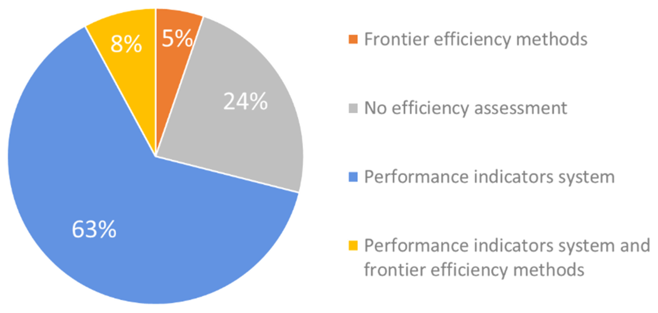
Efficiency methods are widely used in the water sector to assess the relative efficiency of utilities and promote competitiveness [4]. In order to determine the specific tools water regulators use to assess efficiency, the authors conducted a survey. This survey was sent to 141 water regulatory authorities around the world, and was answered by 27% of them. The results include regulators from 28 different countries located in America, Europe, and Africa. Some of them are regional water regulators, while others regulate at the national level. Figure 1 shows the answers to the question regarding the tools of choice for water regulators to assess the efficiency of utilities.
Figure 1 reveals that although performance indicator systems are the preferred methods for assessing efficiency in regulated water sectors, frontier efficiency methods represent a significant proportion at 13%. This work is focused on the latter, and more specifically on two methods—econometric and non-parametric frontier efficiency methods. The aim of these methods is to obtain an efficiency frontier and use it for comparison against the performance of utilities, thereby determining their degree of inefficiency.
There are plenty of studies on frontier efficiency methods applied to water distribution systems (e.g., [5,6]). These methods are used to compare the efficiency of water utilities and analyze any drivers affecting this (e.g., economies of scale and scope, public vs. private operation, or the effect of regulation in efficiency and productivity [5]). These references use a wide range of methods, model configurations, and variables, depending on what is being analyzed. The literature shows that results are highly dependent on the context of the sample and the methodology employed.
Furthermore, very few studies have been carried out to determine the impact of data quality on results or to determine whether the limited number of variables a model can handle is enough to completely characterize water utilities and determine their efficiency.
Despite some reasonable doubts about their adequacy, frontier efficiency methods have been and are being used by water sector regulators, as shown in Figure 1. These methods are often used in tariff-setting processes by regulators such as OFWAT (Office of Water Services—England and Wales) or the Danish Competition and Consumer Authority (the Danish regulator under the Ministry of Industry, Business, and Financial Affairs [7,8]).
The main benefits of these methodologies are that they do not introduce any bias when assessing the utilities’ performance, as results do not rely on the opinion of the regulator’s expert analysts. Additionally, they reduce the resources needed to regulate the market compared to detailed analyses of performance [9].
This paper analyzes if these methodologies are appropriate for regulating the efficiency of the water sector, and more specifically, for water distribution services. For this purpose, the study will try to determine the impact that some factors may have on the results from a regulatory perspective.
Firstly, the impact of real data quality on the two frontier efficiency models will be determined (the water sector is well-known for data inaccuracies resulting from the nature of its assets). In order to achieve this, a real and audited dataset (with information on the quality of data) will be used to test the methods.
Secondly, the paper will explore further limitations of these methods. As the literature suggests, these models have limitations relating to the maximum number of variables they can consider [10]. The paper will try to determine if the methods can cope with all the variables needed to properly evaluate the utilities’ efficiency. Variables used will include the quality of service aspects expected by users according to ISO 24,510 [11] and the exogenous characteristics that differentiate utilities (such as topography and size).
Finally, the consistency of both methods will be compared to determine their appropriateness as regulatory tools.
2. Methods
There are numerous methods and variants of efficiency models. However, they can be grouped into two main families—econometric (e.g., ordinary least squares (OLS) modified least squares (MLS), stochastic frontier analysis (SFA)) and nonparametric (data envelopment analysis (DEA)). This paper analyzes the ability of DEA and SFA models to assess the efficiency of water utilities (one from each family). The selection of these two models is based on the fact that they have been widely applied in the water sector [6,12] for regulatory purposes [8,13]. Input and cost minimization approaches are used for DEA and SFA, respectively, as it was assumed that water companies aim to minimize their inputs or costs.
DEA is a non-parametric method that uses mathematical programming to obtain efficiency scores of a set of individuals, called decision making units (DMUs), for water utilities. The method identifies the most efficient utilities, locates them in the efficiency frontier, and compares the remaining utilities against this frontier. The DEA model used in this paper was run with General Algebraic Modeling System (GAMS) software, which is a high-level modeling system for mathematical optimization.
The main benefits of DEA are that it does not require any assumption concerning the shape of the frontier and it allows for multiple inputs and outputs [4,10]. In addition, the weights of inputs and outputs are determined intrinsically by the model, reducing any subjective interpretation. The optimal input and output weights are obtained by solving the mathematical programming, so the efficiency of the underevaluated unit is maximized. In other words, the objective function of the optimization model is to maximize the efficiency score by selecting the most desirable weights for inputs and outputs [14]. As a disadvantage, DEA is sensitive to outliers and data uncertainty, although some authors have proposed improvements to tackle this issue [15].
The linear programming model used to estimate the efficiency of several water companies in our study is described below.
Let us assume that j water companies exist in the industry that use a set of inputs xn where n = 1, …, N to generate a set of outputs ym, where m = 1, …, M. The linear programming model is written as follows:
where φ is the efficiency score, which presents the contraction of inputs required so that a unit can be included in the efficiency frontier, λ is the intensity variable used to build the frontier, and the equality ensures that the model is ran under variable returns to scale (VRS).
Parametric or econometric methods have also been used for regulation in the water sector. For instance, OFWAT (Office of Water Services) has employed them to calculate the efficiency of English and Welsh utilities and set their tariffs according to the results [7]. The Danish Competition and Consumer Authority uses them together with a DEA approach to assess the efficiency of the regulated water utilities. According to Berg and Marques [16], 58% of studies performed in the water sector are parametric.
These methods estimate the efficiency frontier following a predetermined function (linear, quadratic, logarithmic, etc.) [4] and determine the efficiency of the sample against the estimated frontier. They can be deterministic (e.g., ordinary least squares (OLS) or corrected ordinary least squares (COLS)) or stochastic. In the first case, the difference between the frontier and the efficiency score is entirely attributed to the inefficiency of the utility. The aim of the latter is to separate inefficiency from random errors, which are those outside the control of the utility, such as droughts and data measurement errors [17].
The econometric method used in this study (stochastic frontier analysis, (SFA)) is a stochastic method, as its name suggests. Its main benefit is allowing separation of the error term from the inefficiency. However, in order to properly formulate the problem, there is an elevated number of decisions to be made beforehand (such as the functional form of the frontier [4]). The SFA model used for this paper was simulated with LIMDEP, an econometric and statistical software package.
SFA is a parametric efficiency analysis approach that assumes a Cobb–Douglas, log-linear, or translog functional form for the underlying technology [18,19]. Following past studies ([20,21,22] and others) a Cobb–Douglas functional form is employed, as the study sample is small and this method does not need many degrees of freedom compared to the translog functional form. The estimated cost frontier takes the following form:
where j denotes the number of water companies (observations); C is the total cost of any company j, which is a function of the output y and environmental variable (quality of service) z; β is the estimated parameter; ν presents random noise; and u is the cost inefficiency, which follows the exponential distribution [23,24]. The cost efficiency of any company j (CEj) in the sample is then calculated as In this study the volume of water delivered, the number of connections, and the length of mains are used as proxies for density. Additional cost drivers are used to capture the quality of service, such as volume of water loss and the number of water service interruptions. Similar variables were also employed in Murwirapachena et al. [22] in the context of water and in Kuosmanen [25] and Jamsbab et al. [26] in the electricity sector.
This work explores the sensitivity of both methods to uncertain data and their limitations, especially their response to an elevated number of variables. The consistency of the methods is of special interest for regulatory purposes (i.e., if utilities obtain similar results regardless of the method or the data uncertainty), as utilities could argue whether the calculated efficiency is in fact real or a method dependent. For this reason, the paper will also focus on how the efficiency score and the position in the ranking may vary depending on the data and methods used.
Description of the Sample
The sample used to conduct the empirical application is a 2015 dataset collected by ERSAR (the Portuguese water and wastewater regulatory authority) [27]. This dataset was selected because the data were publicly available, they were audited by ERSAR, and all variables had an uncertainty band associated, reflecting the quality of data (e.g., if the data from the utility water meters have 0%–5% uncertainty, this means that the reported value could be up to 5% greater or smaller).
The data sample was chosen considering that reliable data in the water sector are very scarce. The data published by ERSAR are the only data in the world that are publicly available, validated by a third party, and contain information on the uncertainty of each data element.
The results of this work are focused on evaluating whether frontier efficiency methods (and more specifically DEA and SFA) are adequate tools for the regulation of water services. The analysis of the results has a global application and the origins of the dataset used do not limit the validity of the results from a geographical point of view.
From the 265 water utilities in the actual dataset, 194 were selected for the study, as the data uncertainty information for the remaining ones was incomplete. All 194 utilities provide water supply services, although some of them are multi-utilities, providing other services such as wastewater.
Uncertainty in the dataset is recorded in the following tolerance bands: 0%–5%, 5%–20%, 20%–50%, 50%–100%, 100%–300% and >300%. Most variables in the dataset fell under the 0%–5% and the 5%–20% tolerance bands. However, some utilities reported uncertainties for some variables between 50% and 100%, or even up to 300% (the uncertainty band is reported by the utility to the regulator and may be externally audited).
Regarding the selection of variables, following Marques et al. [28], three criteria were considered: (i) the particularities of the water industry; (ii) the actual data elements available in the Portuguese dataset, and (iii) examples in the literature [16,29].
The variables used for both DEA and SFA models were network length (km), total expenses (€/year), volume of real water losses (m3/year), service interruptions (number/year), volume of produced water (m3/year), and number of households covered by the water service (No.). The description of each variable can be found in the ERSAR Technical Guide [30]. Table 1 summarizes the use of these variables in each model.
All these variables have been extensively cited in literature for use in assessing the performance of water utilities [5,6], the exception being the total expenses, which were selected instead of the operating and manpower costs (the typical variables used for these studies). Total expenses, which include capital and operating expenses, are not commonly used due to the discrepancies in this valuations between utilities. However, in this case, the data come from a regulated environment, guaranteeing that all utilities calculate this variable following the same definition and procedure, and results are, thus, comparable. Table 2 reports the descriptive statistics of the variables used in the study.
3. Impacts of Data Quality and Uncertainty
3.1. General Considerations
The water sector is well-known for having low-quality and uncertain data. There are several factors that contribute to this fact. Firstly, most water networks were built a long time ago (many are over 100 years old), and as the networks are mainly buried, there may be high uncertainty concerning the location, characteristics, and state of at least some of the network’s assets. Secondly, there are variables that cannot be measured accurately at a reasonable cost. For instance, domestic water meters are required by standards to keep their error below 2% in steady flow and 5% in transition flow [31]. However, these measurement errors correspond to brand new meters that have been properly selected for each type of use, and in practice errors can be significantly higher [32]. Finally, there are variables which are not measured but rather calculated, including estimated values (e.g., water losses). In these cases, the uncertainty is even greater, as several uncertainties are combined or estimations are included.
These uncertainties are not avoidable; rather, they are intrinsic to the water sector (with the current technology they can be reduced but not completely eliminated). This is why the Manual of Best Practice for performance indicators of the IWA (International Water Association) stresses the need to consider data quality as part of any performance assessment system [33,34]. If input variables cannot be limited to a single value, but rather include a range of values, it seems logical that econometric methods should include a range of outputs rather than being limited to a single output.
3.2. Data Envelopment Analysis Model
The impact of data quality on the results of a DEA model were explored in detail by the authors in a previous paper [35], and a brief summary with the major findings is included below in order to compare them to SFA results.
In order to determine the impact of data uncertainty on the results, a DEA tolerance approach was used with the described dataset. A tolerance interval was established for each variable to account for uncertainty (as variables could actually take any value within this interval). Following Molinos-Senante et al. [35], 81 (34) DEA scenarios were run with different combinations of values for variables. The three are the alternatives which correspond to the situations considered for each utility (DMU): favorable, unfavorable, and original. The number four are the possible combinations of inputs and outputs were used for the analyzed utility. These are inputs and outputs for the analyzed DMU and inputs and outputs for the remaining DMUs. Thus, the best case scenario for the evaluated utility is has the lowest values for inputs and the highest for outputs.
The results of 81 simulations in the DEA tolerance model with the complete sample of 194 utilities showed a wide range of variability in the efficiency, similar to the results presented by Cabrera et al. [36]. Specifically, the average change in the efficiency of the utilities due to data uncertainty was 71%, reaching 97% for the worst case. As regulators usually base their yardstick regulation approach on the ranking of utilities from best to worse, the impact this change in efficiency had on the ranking was also analyzed. Based on the efficiency scores, the DMUs (water utilities) were ranked. The average variation in ranking was 103 positions, with a maximum variation of 193 positions (out of 194).
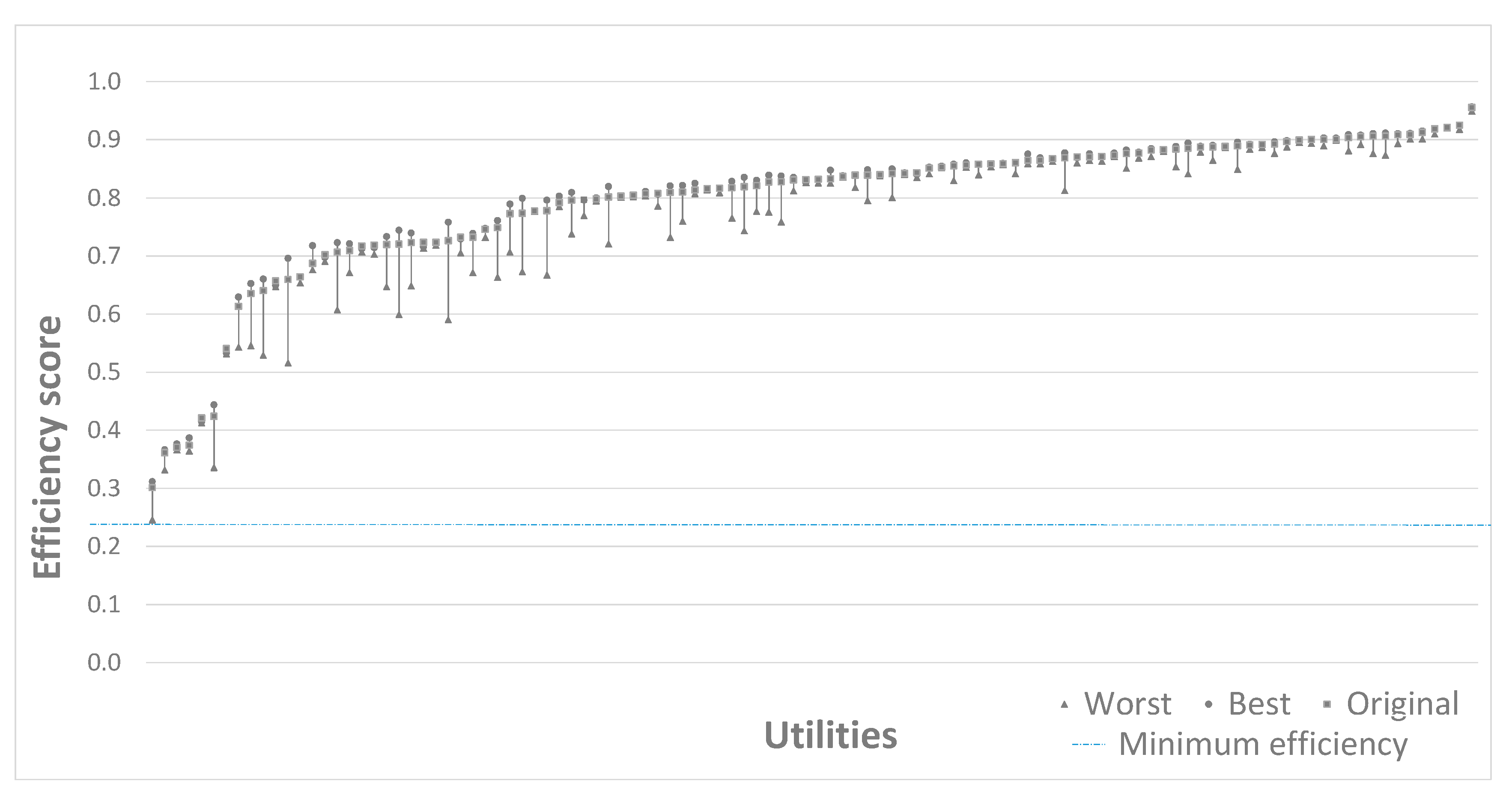
Given the results and the high uncertainties that some utilities showed for some variables, a second DEA tolerance run was performed with a reduced set of utilities [36]. DEA is very sensible to outliers, and therefore these high uncertainties have a relevant effect on the results, as they may impact the frontier and the efficiency scores of all utilities. In this second simulation, utilities with more than 20% uncertainty in any of their variables were removed from the sample. As a consequence, the reduced sample contained 108 utilities. The results in this second sample, as expected, had less variance. Figure 2 displays the results of this simulation. This figure represents the maximum and minimum efficiencies obtained by utilities from the 81 simulations and their original scores. The original DEA score corresponds to the DEA simulation without considering data uncertainty.
As this figure shows, even in this case the variability was still large, with the average change in efficiency being 17% and the highest variability being 43%. Concerning ranking positions, on average utilities changed 13 positions in the ranking, with 49 positions being the maximum change. These results demonstrate how sensible DEA is to uncertain data. This is particularly relevant if results are to be used for regulatory purposes. The results of the 81 simulations for both complete and reduced samples are available in the Supplementary Data File.
These results demonstrate the relevance of the collection, validation, and consideration of data quality when assessing the performance of utilities. DEA is a consistent method as long as data are not uncertain, which is not the case for the water sector. In addition, the resources needed to reduce such uncertainty are considerable, which raises questions about the validity of this method as a regulatory tool for the water sector.
3.3. Stochastic Frontier Analysis Model
In order to provide a more complete picture for this paper, the DEA experiment was repeated with a parametric frontier efficiency method—the SFA method. This required some minor adjustments. There is no equivalent of the DEA tolerance approach in SFA. Therefore, the cases needed to be created manually. Two case scenarios were created in addition to the “original scenario” in order to assess the variability that data quality had on efficiency results. The original scenario does not consider data uncertainty. The two additional cases were built as follows. In one case all variables were set to their most favorable value (e.g., losses and costs set to minimum values), while in the other case they were set to their most unfavorable value. It must be stressed that this is only a minimum sample of the variability for this dataset, as it is very unlikely that the values of all variables for all utilities would actually present their best or worst values in unison.
The SFA case was performed with the reduced and most accurate set of utilities (108 in total). Using the data from all 194 utilities was impossible due to convergence issues in the SFA model. Considering that these data are from a regulated environment where data quality is actually recorded, this raises questions about the practicality of using SFA as a regulatory method in some environments.
The Appendix A (Table A1, Table A2 and Table A3) shows the econometric results from the estimation of the cost frontier model for the three case scenarios: original, best, and worst scenarios. The coefficient of the variables is interpreted as elastic, because the data were normalized around their mean [24]. Output variables are significant across the three models, with volume of water delivered and connections being the major cost drivers, as shown by their coefficients. Technical speaking, if all other factors remain equal, a 1% increase in total expenses may lead to an increase of 0.789%, 0.287%, and 0.145% in the volume of water delivered, connections, and length of mains, respectively. As for the environmental variables, water losses had a statistically significant impact on total costs, which is consistent across models.
Figure 3 displays the results obtained (the detailed complete results are available in the supplementary data file). As this figure shows, none of the utilities are included in the efficiency frontier (efficiency = 1). Additionally, there is less variability of results compared to the DEA study. This is due to the lower effect outliers have in this model, but also a result of the methodology followed to create the cases, especially the best scenario. The scenario considered for each variable is its best performance (from within the variable’s tolerance range). As a result, for most variables the best value is the one with the lowest tolerance value. In those cases where the tolerance band ranges from 0% to 5%, there is no variation from the original scenario (value + 0% tolerance), giving similar results for the two considered scenarios.
In any case, the average variability of efficiency is 8%, and the average variation in the ranking position is higher than 8 positions (as in the DEA model, ranking is obtained from the efficiency scores for utilities, which are obtained from the simulations). The maximum variability in efficiency is 23%, and the maximum change in the ranking is 25 positions. Table 3 displays the variation in the ranking for some utilities.
These results are slightly better than those of the DEA simulation with the reduced dataset. However, considering that the larger set could not be studied with SFA and the number of evaluated options was also smaller, this still raises significant questions about the convenience of SFA as a regulatory tool. After all, the results shown in Table 3 would make a great argument for a regulated utility when trying to discredit the methodology used by the regulator and the conclusions obtained about which utility provides a better, more efficient service.
4. Further DEA and SFA Limitations
Besides the clear impact of data uncertainty on these methods, further limitations should be explored when considering their use for regulatory purposes.
4.1. Limitation of the Number of Variables
As previously stated, econometric methods are limited by the maximum number of variables they can consider. This has not been an obstacle in the applications of the methods reported in the literature, as the number of variables has always been kept within the limits, as seen in the recompilations of frontier efficiency studies from Abbot et al. [5] and Ferro et al. [6].
However, quality of service variables are often overlooked or simplified in these studies. This is critical, as the cost of the service and its quality are intrinsically linked [37], with a consequent impact on efficiency. In other words, if the quality of service provided is not properly considered, a better (and more expensive) service may be considered more inefficient than a worse (but cheaper) service.
The number of quality of service variables in the water sector is higher than in other sectors (e.g., gas or electricity). This implies that more variables need to be assessed and considered when evaluating the kind of service the users are provided. Table 4 displays a list of users’ expectations (corresponding to quality of service variables) for the gas, electricity, and water sectors. User expectations for water are based on ISO standard 24510:2007 [11], while the rest were compiled by the authors of [9].
Frontier efficiency methods have been traditionally used for energy and gas regulation, and were later applied to the water sector [38]. As the number of quality of service aspects to be considered in the water sector is greater, it has to be assessed whether these models can deal with all the variables needed to fairly assess the efficiency of utilities.
In addition to the quality of the service, there are exogenous aspects outside the control of the utilities that have an impact on costs and efficiency (e.g., weather, topography, raw water quality, water sources, population density). These aspects can be estimated by SFA models as random errors, but not by DEA.
Worthington [17] shows how, on average, the number of variables in these models is usually less than 10 (inputs and outputs or dependent and independent variables).
For DEA, there is a rule that fixes the maximum number of inputs and outputs according to the number of DMUs analyzed. This is called Cooper’s rule, , where n is the number of DMUs, m is the number of inputs, and s is the number of outputs [10].
This rule is a limitation for DEA models when the number of utilities assessed is low, such as the DEA model referred to in the previous section, which has 4 inputs and 2 outputs, requiring a minimum of 18 DMUs. A DEA model considering all the user expectations from ISO standard 24510, in addition to context information (topography, etc.), would require even more utilities.
As an example, let’s suppose that in addition to the 6 variables used in the previous chapter, the following inputs are considered: the infrastructure value index (IVI), as a measure of the sustainability of the infrastructure; the average pressure in domestic connections; the percentage of water quality tests passed; and the average topographic elevation of the network. Additionally, the following two explanatory variables are considered as inputs as well: customer satisfaction and type of water source. In this case, the number of minimum DMUs would increase to 36. This is not a problem in the specific dataset from the Portuguese water sector, as the number of utilities is large, but this is a limitation in areas with fewer utilities, such as the United Kingdom, the Netherlands, or Australia.
The selection of variables in the SFA is more delicate, as the dependent variable has to be expressed as a function of the independent variables. When selecting the variables, a basic descriptive analysis should always be performed in order to detect possible sources of errors in the model, such as heteroscedasticity or multi-collinearity (at least 2 variables are highly linearly related).
There is no maximum number of independent variables that should be used in a SFA model. This number depends on the degrees of freedom of the model and the number of observations (in our case, number of utilities). If there are few observations and the number of variables is high, there will not be enough degrees of freedom left and the model will not work properly.
Therefore, in both the DEA and SFA models, the number of variables admitted depends on the size of the sample. In large samples, such as the Portuguese sample used previously, the model could admit as many variables as needed, while in smaller samples (e.g., the UK) there is a limitation and most quality of service or context variables will be discarded.
However, a larger number of utilities is not the only answer to the problem, as the more variables the model has, the more likely it is to have multi-collinearity problems between those variables. Multi-collinearity is usually present in samples from the water sector [17], and models with a larger number of variables are more likely to have this. There is evidence that if the correlation between variables is higher than 0.8, the model can be biased and results of the model can be affected, especially in SFA [39]. Possible solutions include enlarging the sample (difficult in a regulated environment, as it would require the number of utilities assessed with the model to be increased) or reducing highly correlated variables, although in the latter case, the problem of misspecification in the model [39] could appear, misrepresenting reality.
4.2. Other Limitations of Frontier Efficiency Methods for Regulatory Uses
As established in The Lisbon Charter [40], any regulatory body should be based on the principle of transparency. One of the responsibilities of these bodies, according to this charter, is “providing reliable, concise, credible information that can be easily interpreted by all, covering all operators, regardless of the management system adopted for service provision.” Frontier efficiency methods may not be the best suited for regulation based on these principles. As complex methods, the average citizen does not understand the process followed to rank utilities and make regulatory decisions. As a result, users need to trust the regulatory experts and believe the process followed is the most appropriate for the task. This is not ideal, and when the regulator changes each price review method, users may question the validity of the results from previous reviews, as could be the case for OFWAT [7,13,41,42].
The selection of variables is another key part of the process (DEA is particularly sensitive to variable selection [17]). This is not trivial, since there are many variables to select from, as previously stated. Abbot and Cohen [5] and Ferro et al. [6] published reviews of frontier efficiency methods applied to the water sector. An analysis of the inputs, outputs, and environmental variables of these reviews shows that there are more than 20 different variables considered in the literature as inputs, 45 as outputs, and 30 as environmental variables. The selection of variables will determine the adequacy of the model and has to be related to the sample’s context. The expertise and knowledge of the water sector is needed for proper selection of variables and to accurately model real situations. Since the results will change depending on the variables used, the variable selection may always be disputed by utilities who understand that they would be perceived as more efficient with different variables.
Finally, there are several technical decisions to be made, such as the functional form in SFA or variable and constant returns of scale in DEA [4]. These decisions have direct impacts on the results. According to Worthington [17], there are so many configurations in frontier efficiency models that even with the same model results can widely differ due to their configuration. Once more, this is a serious challenge in their use for regulatory purposes, as those utilities with less favorable efficiency results can argue that results are due to an unfair model that does not entirely capture the context, and could propose similar models with the same variables but different parameters, whereby the utility receives better results [43].
5. Consistency Check of DEA and SFA Models
Few authors have compared the performance of the SFA and DEA approaches to evaluate the consistency of their performance (efficiency and productivity change). Some examples are Kirkpatrick et al. [43], Berg and Lin [44], Molinos-Senante and Maziotis [45], and Corton and Berg [46].
As DEA and SFA methods are based on different principles, their efficiencies can differ [4]. For the purpose of this comparison, results of these methods are considered to be consistent if the efficiencies and rankings are similar and the methods identify the same groups of best and worst performers.
The inconsistency of the results between the two methods has previously been reported in the literature. For instance, a study comparing the performance of six Latin American countries using SFA and DEA found that a utility that was close to the top in the DEA model was the lowest ranked in the SFA model [46].
Another relevant example for water sector regulation is the case of OFWAT. In the previous price review for 2014 (PR14), this regulator obtained the efficiencies of utilities with three different models. The reason was that none of the models was considered to entirely capture the efficiency or to be completely reliable. In addition, the results provided by these models were different. Therefore, in order to minimize the impact of selecting an inaccurate model, the result of each was triangulated to obtain the efficiency score for each utility [7].
This procedure led companies to complain, as they did not consider the models to be accurate enough to act as the baseline for the price review and base tariffs. As argued by Kumbhakar [47], the average of three models when one or more is inaccurate ruins the results from the accurate one, and the efficiency score is likely to be incorrect.
The Danish regulator also performed DEA and SFA simulations in a best-of-two approach [8], a procedure that raises the same questions as in the OFWAT case.
For the purposes of this study, in order to assess the consistency of DEA and SFA methods for regulatory purposes, the differences of the efficiency scores and the positions in the ranking between the original simulation of these two models will be compared. For this comparison it will be used the reduced sample of 108 utilities described previously.
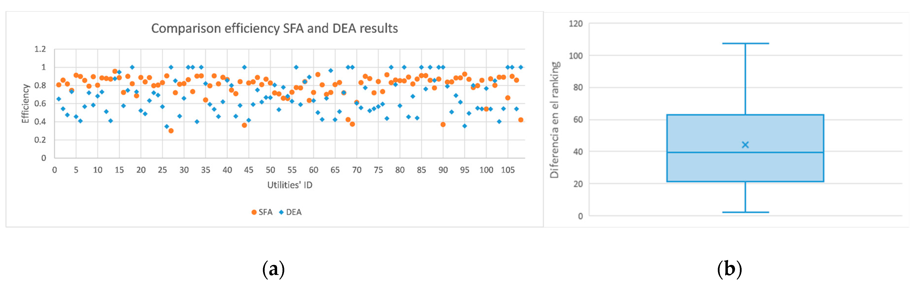
As can be observed in Figure 4a, utilities generally show better efficiencies when evaluated with the SFA, although when using DEA efficiencies are more disperse. None of the utilities under the SFA model reaches the efficiency frontier, whereas in the DEA model, 18 utilities reach the frontier. Concerning the lowest efficiencies, both methods have efficiencies as low as 35%. The average efficiency for SFA is 79%, whereas the average efficiency for DEA is slightly lower at 68%. This difference is not surprising as, SFA generally obtains better efficiencies than DEA [39].
As previously mentioned, regulators using frontier efficiency methods for yardstick regulation generally use ranking positions rather than the efficiency score itself. Therefore, although SFA and DEA models may provide different efficiency scores for utilities, if ranking positions were similar, results would be probably be acceptable (and could be considered consistent).
The variation in the ranking position obtained with each model was compared. On average, utilities had a variation of 44 positions in the ranking between both models, with a maximum variation of 107 positions (out of 108) and a minimum of 2 positions. As seen in Figure 4b, utilities occupying the central 50% of the sample change between 21 and 62 positions. These outcomes suggest that results from DEA and SFA are not consistent, as they do not identify the same group of utilities as good or bad performers. In other words, utilities that are considered good performers by one method do not receive the same result from the other. Consequently, the use of these methods for regulation could be questioned by utilities.
As suggested by Molinos-Senante and Maziotis [45], the deviations between SFA and DEA results are firstly due to the fact that the SFA requires a functional form for the unknown technology, which DEA does not, as it is a deterministic approach. Secondly, the DEA method is more sensitive to data variation than the SFA method.
Additionally, part of the difference in results between both methods may be due to the fact that SFA separates inefficiency into real inefficiency and random effects. Thus, any differences in the efficiency results between DEA and SFA could be attributed to the assumptions implied by these two methods.
However, with no further data concerning the context of utilities, it is not possible to know if there is any other reason for these differences and comparisons between both methods are inconclusive. An extensive analysis of the context and external factors affecting water utilities would be needed in order to determine the reason behind the discrepancies between methods.
6. Conclusions
This paper analyzed the adequacy of frontier efficiency methods for the regulation of the water sector, and more specifically DEA and SFA. Their adequacy was assessed based on three aspects: (i) how they behave with the uncertain data from the sector; (ii) how other limitations affect their use for regulatory purposes; and (iii) the consistency of the results obtained with both methods.
Results show that DEA is very sensitive to data uncertainty, and therefore the ranking of utilities will be affected by normal data variations within the range data of uncertainty. The SFA model shows less variance, although it is still significant.
The number of variables to be considered in order to fully evaluate the efficiency of a water utility for regulatory purposes is large, as the quality of service and the utility’s context need to be characterized. It has been found that in both models, if a large set of variables is to be modelled, the size of the sample (number of utilities) also has to be large. For DEA, Cooper’s rule has to be fulfilled. For SFA, the degrees of freedom must be preserved. Even for large samples where many variables can be considered (as in this study), issues of multi-collinearity between the variables may appear. When the number of utilities is low, the number of variables will be a limitation for assessing efficiency with these methods.
These methods are hard to understand for the average user, and they represent a barrier between the regulator and the users, discouraging public participation and interest in the regulatory process.
Finally, there are important differences in the efficiency values and ranking positions obtained with both methods, something that is further confirmed by other examples in the literature. This lack of consistency may have a significant impact on the credibility of the results, especially when considered as regulatory tools.
In consequence, the use of these methods for regulatory purposes may not be recommendable, as the decisions made based on them can be questioned by utilities and users.
This conclusion does not call into question the validity of the methodologies, which has been extensively demonstrated in the literature. However, the specific conditions of the water sector have a direct and noticeable impact on the results.
The results obtained with frontier efficiency methods often constitute the start of the conversation between the regulator and utilities, and not the ultimate criteria for making decisions. However, the results should not be considered infallible and a consideration should be made for less complex and transparent methods that can also encourage efficiency and promote a similar dialogue between the regulator and the utilities.
Supplementary Materials
The materials are available online at https://www.mdpi.com/2073-4441/12/4/1046/s1.
Author Contributions
Conceptualization, E.E.-J. and E.C.J.; investigation, E.E.-J., M.M.-S. and A.M.; methodology, E.E.-J., M.M.-S. and A.M.; supervision, E.C.J.; writing—original draft, E.E.-J.; writing—review & editing, E.C.J. All authors have read and agreed to the published version of the manuscript.
Funding
This research received no external funding.
Conflicts of Interest
The authors declare no conflict of interest.
Appendix A

Table A1.
Estimates of the cost frontier model for the original scenario.
| Variables | Parameter | Coefficient | Standard Error | T-Statistic | p-Value |
|---|---|---|---|---|---|
| Constant | β0 | 4.165 | 0.864 | 4.823 | 0.000 |
| Water delivered | β1 | 0.789 | 0.111 | 7.098 | 0.000 |
| Connections | β2 | 0.287 | 0.108 | 2.650 | 0.008 |
| Network length | β3 | 0.145 | 0.053 | 2.718 | 0.007 |
| Service interruptions | β4 | 0.003 | 0.024 | 0.117 | 0.907 |
| Water losses | β5 | −0.285 | 0.064 | −4.486 | 0.000 |
| Log-likelihood | −31.839 | ||||
| Theta | 4.020 | 0.749 | 5.366 | 0.000 | |
| Sigmav | 0.228 | 0.029 | 7.848 | 0.000 |
Dependent variable = total expenses. Sigmav is the Standard deviation of v. Bold coefficients are statistically significant from zero at the 5% level.
Table A2.
Estimates of the cost frontier model for the best scenario.
| Variables | Parameter | Coefficient | S.E. | T-Statistic | p-Value |
|---|---|---|---|---|---|
| Constant | β0 | 4.420 | 0.926 | 4.775 | 0.000 |
| Water delivered | β1 | 0.800 | 0.117 | 6.832 | 0.000 |
| Connections | β2 | 0.303 | 0.112 | 2.693 | 0.007 |
| Network length | β3 | 0.167 | 0.057 | 2.951 | 0.003 |
| Service interruptions | β4 | −0.002 | 0.026 | −0.075 | 0.940 |
| Water losses | β5 | −0.305 | 0.068 | −4.468 | 0.000 |
| Log-likelihood | −42.116 | ||||
| Theta | 3.473 | 0.667 | 5.207 | 0.000 | |
| Sigmav | 0.241 | 0.036 | 6.738 | 0.000 |
Dependent variable = total expenses. Sigmav is the Standard deviation of v. Bold coefficients are statistically significant from zero at the 5% level.
Table A3.
Estimates of the cost frontier model: worst scenario.
| Variables | Parameter | Coefficient | S.E. | T-Statistic | p-Value |
|---|---|---|---|---|---|
| Constant | β0 | 4.037 | 0.848 | 4.762 | 0.000 |
| Water delivered | β1 | 0.780 | 0.109 | 7.122 | 0.000 |
| Connections | β2 | 0.286 | 0.107 | 2.667 | 0.008 |
| Network length | β3 | 0.138 | 0.052 | 2.631 | 0.009 |
| Service interruptions | β4 | 0.004 | 0.023 | 0.155 | 0.877 |
| Water losses | β5 | −0.276 | 0.062 | −4.418 | 0.000 |
| Log-likelihood | −29.887 | ||||
| Theta | 4.094 | 0.751 | 5.450 | 0.000 | |
| Sigmav | 0.224 | 0.028 | 8.010 | 0.000 |
Dependent variable = total expenses. Sigmav is the Standard deviation of v. Bold coefficients are statistically significant from zero at the 5% level.
References
- Posner, R.A. Natural Monopoly and Its Regulation. Stanf. Law Rev. 1969, 21, 548. [Google Scholar] [CrossRef] [Green Version]
- Shleifer, A. A Theory of Yardstick Competition. RAND J. Econ. 1985, 16, 319. [Google Scholar] [CrossRef]
- Coelli, T.; Walding, S. Performance measurement in the Australian water supply industry: A preliminary analysis. In Performance Measurement and Regulation of Network Utilities, 1st ed.; Edward Elgar Publishing Limited: Cornwall, UK, 2006. [Google Scholar]
- Ferro, G.; Lentini, E.; Romero, C.A. Eficiencia y su Medición en Prestadores de Servicios de Agua Potable y Alcantarillado. Available online: http://hispagua.cedex.es/sites/default/files/hispagua_documento/documentacion/documentos/eficiencia_agua_potable_alcantarillado.pdf (accessed on 10 December 2019).
- Abbott, M.; Cohen, B. Productivity and efficiency in the water industry. Util. Policy 2009, 17, 233–244. [Google Scholar] [CrossRef]
- Ferro, G.; Lentini, E.J.; Mercadier, A.C.; Romero, C.A. Efficiency in Brazil’s water and sanitation sector and its relationship with regional provision, property and the independence of operators. Util. Policy 2014, 28, 42–51. [Google Scholar] [CrossRef]
- CEPA (Cambridge Economic Policy Associates Ltd.). OFWAT: Cost Assessment—Advanced Econometric Models. Available online: https://www.ofwat.gov.uk/wp-content/uploads/2015/11/rpt_com201301cepacostassess.pdf (accessed on 20 May 2017).
- Forsyningssekretariatet. Total Economic Benchmarking—Determination of Individual Efficiency Requirements in the Financial Framework for 2018–2019 for Water and Wastewater Companies; Forsyningssekretariatet: Copenhagen, Denmark, 2017. [Google Scholar]
- Cabrera, E., Jr. The need for the regulation of water services. Key factors involved. In Regulation of Urban Water Services. An Overview; Marcet, E.C., Cabrera, E., Jr., Eds.; IWA Publishing: London, UK, 2016; p. 218. [Google Scholar]
- Cooper, W.W.; Seiford, L.M.; Zhu, J. Handbook on Data Envelopment Analysis; Springer: Berlin/Heidelberg, Germany, 2011. [Google Scholar]
- ISO. Activities Relating to Drinking Water and Wastewater Services—Guidelines for the Assessment and for the Improvement of the Service to Users; ISO Copyright Office: Geneva, Switzerland, 2007. [Google Scholar]
- Byrnes, J.; Crase, L.; Dollery, B.; Villano, R.A. The relative economic efficiency of urban water utilities in regional New South Wales and Victoria. Resour. Energy Econ. 2010, 32, 439–455. [Google Scholar] [CrossRef]
- Thanassoulis, E. The use of data envelopment analysis in the regulation of UK water utilities: Water distribution. Eur. J. Oper. Res. 2000, 126, 436–453. [Google Scholar] [CrossRef]
- Yekta, A.P.; Kordrostami, S.; Amirteimoori, A.; Matin, R.K. Data envelopment analysis with common weights: The weight restriction approach. Math. Sci. 2018, 12, 197–203. [Google Scholar] [CrossRef] [Green Version]
- De Witte, K.; Marques, R.C. Influential observations in frontier models, a robust non-oriented approach to the water sector. Ann. Oper. Res. 2010, 181, 377–392. [Google Scholar] [CrossRef] [Green Version]
- Berg, S.; Marques, R.C. Quantitative studies of water and sanitation utilities: A benchmarking literature survey. Hydrol. Res. 2011, 13, 591–606. [Google Scholar] [CrossRef] [Green Version]
- Worthington, A.C. A review of frontier approaches to efficiency and productivity measurement in urban water utilities. Urban Water J. 2013, 11, 55–73. [Google Scholar] [CrossRef]
- Aigner, D.; Lovell, C.; Schmidt, P. Formulation and estimation of stochastic frontier production function models. J. Econ. 1977, 6, 21–37. [Google Scholar] [CrossRef]
- Meeusen, W.; Broeck, J.V.D. Efficiency Estimation from Cobb-Douglas Production Functions with Composed Error. Int. Econ. Rev. 1977, 18, 435. [Google Scholar] [CrossRef]
- Cullmann, A. Benchmarking and firm heterogeneity: A latent class analysis for German electricity distribution companies. Empir. Econ. 2010, 42, 147–169. [Google Scholar] [CrossRef]
- Ferro, G.; Mercadier, A.C. Technical efficiency in Chile’s water and sanitation providers. Util. Policy 2016, 43, 97–106. [Google Scholar] [CrossRef]
- Murwirapachena, G.; Mahabir, J.; Mulwa, R.; Dikgang, J. Efficiency in South African Water Utilities: A Comparison of Estimates from DEA, SFA and StoNED; Economic Research Southern Africa (ERSA): Cape Town, South Africa, 2019. [Google Scholar]
- Saal, D.S.; Parker, D.; Weyman-Jones, T. Determining the contribution of technical change, efficiency change and scale change to productivity growth in the privatized English and Welsh water and sewerage industry: 1985–2000. J. Prod. Anal. 2007, 28, 127–139. [Google Scholar] [CrossRef]
- Molinos-Senante, M.; Porcher, S.; Maziotis, A. Impact of regulation on English and Welsh water-only companies: An input-distance function approach. Environ. Sci. Pollut. Res. 2017, 24, 16994–17005. [Google Scholar] [CrossRef]
- Kuosmanen, T. Stochastic Semi-Nonparametric Efficiency Analysis of Electricity Distribution Networks: Application of the StoNED Method in the Finnish Regulatory Model. SSRN Electron. J. 2011, 34, 2189–2199. [Google Scholar] [CrossRef]
- Jamasb, T.; Orea, L.; Pollitt, M. Estimating the marginal cost of quality improvements: The case of the UK electricity distribution companies. Energy Econ. 2012, 34, 1498–1506. [Google Scholar] [CrossRef] [Green Version]
- ERSAR. ERSAR—Relatório Anual dos Serviços de Águas e Resíduos em Portugal. 2015. Available online: http://www.esgra.pt/ersar-relatorio-anual-dos-servicos-de-aguas-e-residuos-em-portugal/ (accessed on 16 June 2017).
- Marques, R.C.; Berg, S.V.; Yane, S. Nonparametric Benchmarking of Japanese Water Utilities: Institutional and Environmental Factors Affecting Efficiency. J. Water Resour. Plan. Manag. 2014, 140, 562–571. [Google Scholar] [CrossRef] [Green Version]
- Pinto, F.S.; Costa, A.S.; Figueira, J.R.; Marques, R.C. The quality of service: An overall performance assessment for water utilities. Omega 2017, 69, 115–125. [Google Scholar] [CrossRef]
- ERSAR. Guide for the Assessment of the Quality of Water and Waste Services, 3rd Generation of the Assessment System; ERSAR: Lisbon, Portugal, 2011. [Google Scholar]
- ISO. Water Meters for Cold Potable Water and Hot Water—Part 1: Metrological and Technical Requirements; ISO Copyright Office: Geneva, Switzerland, 2018. [Google Scholar]
- Arregui, F.; Cabrera, E.; Cobacho, R.; García-Serra, J. Key factors affecting water meter accuracy. In Proceedings of the Specialised Conference of the IWA, Halifax, NS, Canada, 12–14 July 2005; pp. 1–10. [Google Scholar]
- Matos, R.; Cardoso, M.; Duarte, P.; Ashley, R.; Molinari, A.; Schulz, A. Performance indicators for wastewater services—Towards a manual of best practice. Water Supply 2003, 3, 365–371. [Google Scholar] [CrossRef]
- Alegre, H.; Baptista, J.; Cabrera, E.; Cubillo, F.; Duarte, P.; Hirner, W.; Merkel, W.; Parena, R. Performance Indicators for Water Supply Services: Third Edition. Water Intell. Online 2016, 15. [Google Scholar] [CrossRef]
- Cabrera, E.; Estruch-Juan, E.; Molinos-Senante, M. Adequacy of DEA as a regulatory tool in the water sector. The impact of data uncertainty. Environ. Sci. Policy 2018, 85, 155–162. [Google Scholar] [CrossRef]
- Molinos-Senante, M.; Donoso, G.; Sala-Garrido, R. Assessing the efficiency of Chilean water and sewerage companies accounting for uncertainty. Environ. Sci. Policy 2016, 61, 116–123. [Google Scholar] [CrossRef]
- Picazo-Tadeo, A.J.; Fernandez, F.J.S.; González-Gómez, F. Does service quality matter in measuring the performance of water utilities? Util. Policy 2008, 16, 30–38. [Google Scholar] [CrossRef] [Green Version]
- Marques, R.C.; Contreras, F.H.G. Performance-based potable water and sewer service regulation: The regulatory model. Cuad. Adm. 2007, 20, 283–298. [Google Scholar]
- Dubouskaya, A. Relative Performance of DEA and SFA in Response to Multicollinearity and Measurement Error Problems. Master’s Thesis, National University “Kyiv-Mohyla Academy”, Kiev, Ukraine, 2006. [Google Scholar]
- IWA. The Lisbon Charter; IWA Publishing: London, UK, 2015. [Google Scholar]
- OFWAT. Delivering Water 2020: Our Final Methodology for the 2019 Price Review; OFWAT: London, UK, 2017.
- OFWAT. Setting price limits for 2010-15: Framework and Approach; OFWAT: London, UK, 2008.
- Kumbhakar, S. A Critique of Ofwat’s Cost Assessment Models; Southern water: Worthing, UK, 2014. [Google Scholar]
- Berg, S.; Lin, C. Consistency in performance rankings: The Peru water sector. Appl. Econ. 2008, 40, 793–805. [Google Scholar] [CrossRef]
- Ferro, G.; Romero, C.A. Setting performance standards for regulation of water services: Benchmarking Latin American utilities. Hydrol. Res. 2011, 13, 607–623. [Google Scholar] [CrossRef]
- Molinos-Senante, M.; Maziotis, A. Productivity growth and its drivers in the Chilean water and sewerage industry: A comparison of alternative benchmarking techniques. Urban Water J. 2019, 16, 353–364. [Google Scholar] [CrossRef]
- Corton, M.L.; Berg, S.V. Benchmarking Central American water utilities. Util. Policy 2009, 17, 267–275. [Google Scholar] [CrossRef] [Green Version]
Figure 1.
Methods used by water regulators to assess the efficiency of water utilities.

Figure 2.
Minimum, maximum, and original data envelopment analysis (DEA) results for the reduced sample [36].
Figure 2.
Minimum, maximum, and original data envelopment analysis (DEA) results for the reduced sample [36].

Figure 3.
Minimum, maximum, and original stochastic frontier analysis (SFA) results for the reduced sample.
Figure 3.
Minimum, maximum, and original stochastic frontier analysis (SFA) results for the reduced sample.

Figure 4.
Comparison of the efficiency scores from the reduced sample for SFA and DEA models: (a) efficiency results for both SFA and DEA models: (b) differences in the ranking positions between both methods.
Figure 4.
Comparison of the efficiency scores from the reduced sample for SFA and DEA models: (a) efficiency results for both SFA and DEA models: (b) differences in the ranking positions between both methods.

Table 1.
Configuration of the variables for the data envelopment analysis (DEA) and stochastic frontier analysis (SFA) models.
Table 1.
Configuration of the variables for the data envelopment analysis (DEA) and stochastic frontier analysis (SFA) models.
| Variables | DEA Model | SFA Model |
|---|---|---|
| Network length (km) | Input | Independent/Output |
| Total expenses (€/year) | Input | Dependent |
| Volume of real water losses (m3/year) | Input | Independent/Environmental |
| Service interruptions (number/year) | Input | Independent/Environmental |
| Volume of produced water (m3/year) | Output | Independent/Output |
| Number of households covered by the water service (number/year) | Output | Independent/Output |
Table 2.
Descriptive statistics.
| Variables | Unit | Mean | Standard Deviation | Minimum | Maximum |
|---|---|---|---|---|---|
| Volume of water produced | m3/year | 3,994,778 | 8,971,219 | 133,259 | 107,304,807 |
| Number of households covered by the water service | nr/year | 22,161 | 36,715 | 1157 | 308,986 |
| Network length | km | 448 | 479 | 7 | 3960 |
| Total expenses | €/year | 3,777,639 | 7,114,562 | 0.001 | 72,270,048 |
| Volume of real water losses | m3/year | 751,023 | 975,151 | 8000 | 5,694,343 |
| Service interruptions | nr/year | 15 | 31 | 0.001 | 233 |
| Observations | 194 |
Table 3.
Example of variation of utilities in the ranking.
| ID Utility | Original Simulation | Simulation 1 | Simulation 2 | Max ΔPosition | ||
|---|---|---|---|---|---|---|
| Ranking Position | Ranking Position | ΔPosition | Ranking Position | ΔPosition | ||
| 49 | 34 | 30 |  4 4 | 55 |  −21 −21 | 25 |
| 15 | 24 | 43 | −19 | 19 | 5 | 24 |
| 39 | 20 | 39 | −19 | 18 | 2 | 21 |
| 26 | 8 | 25 | −17 | 6 | 2 | 19 |
Table 4.
Users expectations in gas, electricity, and drinking water or wastewater services.
| Gas | Electricity | Drinking Water/Wastewater |
|---|---|---|
| Continuity | Continuity | Continuity |
| Suitable rates | Suitable rates | Suitable rates |
| Correct customer management | Correct customer management | Correct customer management |
| Suitable voltage/current | Suitable pressure/flow rate | |
| Drinkability | ||
| No taste | ||
| No smell | ||
| No residual flooding | ||
| Minimum environmental impact |
© 2020 by the authors. Licensee MDPI, Basel, Switzerland. This article is an open access article distributed under the terms and conditions of the Creative Commons Attribution (CC BY) license (http://creativecommons.org/licenses/by/4.0/).
Share and Cite
MDPI and ACS Style
Estruch-Juan, E.; Cabrera, E., Jr.; Molinos-Senante, M.; Maziotis, A. Are Frontier Efficiency Methods Adequate to Compare the Efficiency of Water Utilities for Regulatory Purposes? Water 2020, 12, 1046. https://doi.org/10.3390/w12041046
AMA Style
Estruch-Juan E, Cabrera E Jr., Molinos-Senante M, Maziotis A. Are Frontier Efficiency Methods Adequate to Compare the Efficiency of Water Utilities for Regulatory Purposes? Water. 2020; 12(4):1046. https://doi.org/10.3390/w12041046
Chicago/Turabian StyleEstruch-Juan, Elvira, Enrique Cabrera, Jr., María Molinos-Senante, and Alexandros Maziotis. 2020. "Are Frontier Efficiency Methods Adequate to Compare the Efficiency of Water Utilities for Regulatory Purposes?" Water 12, no. 4: 1046. https://doi.org/10.3390/w12041046
Note that from the first issue of 2016, this journal uses article numbers instead of page numbers. See further details here.