A Two-Dimensional Depth-Averaged Sediment Transport Mobile-Bed Model with Polygonal Meshes


Technical Service Center, U.S. Bureau of Reclamation, Bldg. 67, P.O. Box 25007, Denver, CO 80225, USA
Water 2020, 12(4), 1032; https://doi.org/10.3390/w12041032
Submission received: 6 March 2020
/
Revised: 31 March 2020
/
Accepted: 1 April 2020
/
Published: 4 April 2020
(This article belongs to the Special Issue Multi-Dimensional Modeling of Flow and Sediment Transport)
Abstract
:A polygonal-mesh based numerical method is developed to simulate sediment transport in mobile-bed streams with free surfaces. The flow and sediment transport governing equations are depth-averaged and solved in the two-dimensional (2D) horizontal space. The flow and sediment transport are further coupled to the stream bed changes so that erosion and deposition processes are simulated together with the mobile bed changes. Multiple subsurface bed layers are allowed so that bed stratigraphy may be taken into consideration. The proposed numerical discretization is valid for the most flexible polygonal mesh type which includes all existing meshes in use such as the quadrilateral-triangle hybrid mesh. The finite-volume method is adopted such that the mass conservations of both water and sediment are satisfied locally and globally. The sediment transport and stream bed processes are formulated in a general way so that the proposed numerical method may be applied to a wide range of streams and suitable for practical stream applications. The technical details of the numerical method are presented; model verification and validation studies are reported using selected cases having physical model or field measured data. The developed model is intended for general-purpose use available to the public.
1. Introduction
Sediment transport in streams and sedimentation in reservoirs and the associated morphological changes are fundamentally important for the success of many environmental projects. Relevant areas include stream restoration for environmental and ecological benefits, reservoir sedimentation and its sustainability, flood risk management, dam removal, estuary and coastal management, and local scours around, e.g., bridge piers, among many others [1].
One-dimensional (1D) hydraulic flow models have been widely used in practical hydraulic projects for half a century; 1D mobile-bed models have also been developed since and applied in practical projects in the past two decades. Some of the 1D flow and mobile-bed models in wide use include HEC-RAS [2,3], MIKE11 [4], CCHE1D [5], and SRH-1D [6]. 1D mobile-bed models will remain useful for a foreseeable future, particularly for applications with a large spatial extent and/or over a long time period. Their limitations, however, are well known. In recent years, many engineering applications are turning to multi-dimensional models. Among the category, the two-dimensional (2D) depth-averaged models are gaining widespread acceptance due to recent numerical algorithm developments and computer hardware advancements [7,8].
2D depth-averaged flow models have been developed since the works of Chow and Ben-Zvi [9] and Kuipers and Vreugdenhil [10]. 2D mobile-bed models were developed since. Earlier works include Celik and Rodi [11], Spasojevic and Holly [12], Minh Duc [13], Olsen [14], and Wu et al. [15], among others. These early models adopted simple meshes and often assumed local equilibrium in sediment load transport. More general 2D mobile-bed models have been developed since. For example, Wu [16] developed an unsteady model allowing non-uniform and non-equilibrium sediment transport for both suspended load and bedload. The model was tested against several experimental and field cases; good agreements were reported. The model, however, was limited to the structured curvilinear mesh. Hung et al. [17] proposed an implicit two-step operator-splitting method to solve the governing equations. The mesh type was, however, limited to the structured, orthogonal curvilinear coordinate system. Huang et al. [18] developed an adaptive mesh refinement model for dam-break flows over mobile-bed streams. The model was validated against experimental cases with good agreements. The model was limited to the rectangular mesh though adaptation was allowed. At present, there are only a limited number of 2D mobile-bed models which are available to the public for general uses. Such models include CCHE2D [19], TELEMAC [20], UnTRIM [21,22], and Delft3D [23]. CCHE2D was based on the finite element discretization method using the purely quadrilateral or purely triangular meshes; TELEMAC and UnTRIM adopted the purely triangular meshes; and Delft3D was based on the structured mesh. A more flexible mesh version of Delft3D was reported by Kernkamp et al. [24] and used for the suspended sediment modeling in the San Francisco delta and estuary [25]. Orthogonal quadrilaterals, however, were highly recommended according to the developers [26]. In 2D mobile-bed modeling, recent attentions have been on the fundamental formulation issue as discussed by Iverson and Ouyang [27], Cao et al. [28], and Liu et al. [29]. A generally applicable sediment transport formulation is yet to be agreed upon and developed.
Many existing models did not address the unsteady nature of the sediment transport: the quasi-steady assumption has often been made such that the use of the Exner equation were justified [30]. However, a truly unsteady model is not only more general, it is also needed for many processes such as the sediment load travel after a sudden release of sediments due to dam removal or dam failure. Most existing sediment models classified a sediment load into suspended or bed load; but in reality, the transport mode is dependent on local flow conditions and may switch between the two on a natural stream. Further, the switch is not sudden and there usually exist mixed modes in-between the two. Existing sediment models often assumed that the sediment transport rate equaled the sediment transport capacity—the so-called equilibrium assumption. This assumption is appropriate mainly for large spatial and time scales such as 1D modeling; it may fail for event-based sediment transport as well as cases of significant erosion [16]. Some simplifications have been discussed by Cao et al. [28] who pointed out the need for true unsteady and non-equilibrium modeling if a model is intended for general uses. A most significant restriction of the existing models is the adoption of the mesh type which is too restrictive, as reviewed above.
In this study, a 2D depth-averaged mobile-bed model is developed with the aim of the model to be comprehensive and general-purpose. It is being available freely to the public. A major contribution of the present model is the adoption of a general mesh type—the polygon-based mesh—for the sediment transport and mobile-bed modeling. Other new contributions are related to the treatment of the major physical processes: as-general-as-possible approaches are adopted. They include: single sediment transport equation (total load) for all modes (suspended, mixed or bed load); truly unsteady and tightly-coupled formulation of all governing equations, multi-size sediment partition (an arbitrary number of sediment size classes may be used), and non-equilibrium sediment transport. Details of these physical processes are explained below in the governing equations section. The proposed model is applicable to a wide range of environmental stream and reservoir sediment transport modeling issues. To our knowledge, no 2D depth-averaged mobile-bed models have been published that adopts the polygonal meshes.
2. Governing Equations
A 2D depth-averaged mobile-bed model, in general, consists of four interrelated process modules: hydraulic flow, sediment transport, mobile-bed dynamics, and bank erosion. Only the first three modules are described as no bank erosion process is considered in this study. The bank erosion modeling was described by Lai [31] if readers are interested.
2.1. Flow Equations
The flow solver is based on the verified model of Lai [32]. Details may be found from that reference; only the governing equations are presented herein. The 2D depth-averaged flow equations are as follows:
In the above, x and y are horizontal Cartesian coordinates, t is time, h is water depth, and are depth-averaged velocity components in x and y directions, respectively, g is gravitational acceleration, , and are depth-averaged stresses due to turbulence and dispersion, is water surface elevation, is bed elevation, is water density, and and are bed shear stresses. The bed stresses are computed by the Manning’s equation:
where , n is Manning’s coefficient, and is bed frictional velocity. Effective stresses are computed by:
where is kinematic viscosity of water, and is eddy viscosity of turbulence.
The turbulence eddy viscosity needs a turbulence model. Two models are adopted [33]: the depth-averaged parabolic model and the two-equation k-ε model. With the parabolic model, the eddy viscosity is calculated by and the frictional velocity is defined in Equation (4). The model constant may range from 0.3 to 1.0; but the default value of = 0.7 is used in this study. The k-model computes the eddy viscosity by and the two additional partial difference equations for k and ε are solved. The two turbulence equations are not presented herein as the validation cases simulated in this study use the parabolic model only and readers may refer to Lai [32] for further details.
2.2. Sediment Transport Equations
The water column and stream bed are divided into three vertical zones: water column, active layer, and subsurface. Sediments in the water column are transported by flowing water and according to the mass conservation principle. The active layer is a special zone consisting of a thin sediment layer between the water column and the underneath subsurface. Within the active layer, sediment exchange takes place between sediments in the water column and those in the subsurface. The subsurface includes the bed materials underneath the active layer; it may be divided further into multiple subsurface layers so that the vertical variation of sediment composition (stratigraphy) may be taken into account. Physical processes within each zone are different and modeled separately.
Sediments in the three zones may be divided into a user-specified number of size classes, say . In the water column, each size class k is governed by the following single equation no matter the transport mode (suspended, mixed or bed load):
In the above, subscript k denotes that the variable is for sediment size class k, is the depth-averaged sediment concentration by volume, is the sediment-to-flow velocity ratio, is the depth-averaged flow velocity, is the angle of the sediment transport direction relative to x-axis, is the transport mode parameter representing the suspended load fraction, Dx and Dy are the sediment mixing coefficients in the x- and y-directions, respectively, and is the sediment exchange rate between sediments in the water column and those in the active layer or on the bed. The above equation was derived from the mass conservation law by Greimann et al. [30] and took the non-equilibrium nature of a sediment load into account.
The sediment transport angle () may deviate from flow velocity direction due to secondary flows and gravity forces on a transverse bed slope. Several approaches may be used to take these effects into account [34]. In this study, the approach of Struiksma and Crosato [35] is adopted. That is, the angle is computed by:
In the above, is the Shields parameter ( is the bed shear stress,, is the sediment density, is the sediment diameter for size class k), is the particle shape factor, and is the angle of the bed shear stress. The study of Talmon et al. [36] suggested that ranged from 0.5 to 1.0. The bed shear stress angle includes the flow direction and secondary flow effect and is computed by:
In the above, is the von Karman constant (0.41), is the local radius of curvature of flow streamlines, and is a model coefficient (1.0).
The sediment transport mode parameter is introduced to represent the percentage of sediments transported as the suspended load. A similar parameter was introduced by Holly and Rahuel [37] as the “allocation coefficient.” An empirical equation developed by Greimann et al. [30] is used as:
In the above, is the suspension parameter and is the particle fall velocity. If bed load is dominant, is used; is used for suspended load.
The ratio of sediment-to-flow velocity,, was assumed to be 1.0 by most previous studies, which is adequate for many applications. For some applications, such as the unsteady movement of a specified sediment load from a reservoir outlet or a plug, the ratio is not 1.0, and an empirical relation should be developed. In this study, the modified equation of Greimann et al. [30] is used as:
where is the reference Shields parameter (0.045).
The sediment rate term is related to the sediment transport capacity as follows:
In the above, is the sediment transport capacity (volume sediment rate per unit width), is the bed load adaptation length, and is the suspended load parameter.
The sediment transport capacity may be computed with an extensive number of existing sediment capacity or equilibrium equations. Many have been implemented in the present model; but only two are used in the present model verification studies: Engelund and Hansen [38] equation for sandy streams and Parker [39] equation for gravel and mixed sand-gravel streams. The Engelund-Hansen equation is expressed as:
where is the volume fraction of sediment size class k in the active layer. The Parker equation was originally developed for gravel streams but was later found to be applicable also to sand and gravel mixture [40]. The equation is expressed as:
In the above, is the volumetric fraction of the kth sediment size class in the bed, is critical Shield’s parameter, is the medium diameter of the sediment mixture on the bed, and α is the exposure factor. The function in (13a) was fit to the field data and is expressed as:
Parker capacity equation allows two parameters to be defined: and α. represents a critical reference stress above which sediment is mobilized; α is the exposure factor to account for the hiding effect. Hiding is effective for a sediment mixture in which the critical shear stress is reduced for larger particles and increased for smaller particles. Ideally, these two parameters should be fit to available data for a specific stream under simulation. Without site specific data, several references may provide guidance such as Komar [41], Buffington and Montgomery [42], Andrews [40], and Wilcox and Crowe [43]. In general, varies from 0.03 to 0.08 and α from 0.11 to 0.67. In this study, = 0.045 and α = 0.65 are used.
The non-equilibrium bedload adaptation length characterizes the distance for bedload sediments to adjust from a non-equilibrium to equilibrium state; it is related to the scales of the sediment transport, bedform, and stream geometry. It is also a function of the sediment size such that an increase in size leads to a decrease in the adaptation length. A number of methods have been proposed. For example, Thuc [44] applied the sand ripple length, Rahuel et al. [45] used the numerical mesh size, and Wu [16] recommended the dominant length of bedforms such as sand dunes and alternate bars. A review has been conducted by Gaeuman et al. [46]. In the present study, a constant length scale (multiple times of the stream width) is used for gravel streams while the saltation length formula of Philips and Sutherland [47] is used for sandy streams. The Philips-Sutherland equation is expressed as:
where = 0.045 is assumed, and is a model constant with a value of 4000.
Determination of the suspended sediment parameter (ζ) relies on empirical data. Studies [48,49] suggested that a constant ζ ranging from 0.25 to 1.0 might be used and its value depended on whether the bed experienced net deposition or erosion. The recommended value was ζ = 1.0 for net erosion and ζ = 0.25 for net deposition.
Finally, the mixing coefficients, Dx and Dy, include contributions from both turbulence as well as dispersion. For many cases, zero mixing coefficients may be used. Otherwise, the coefficients are set to equal to the turbulent viscosity with the Schmidt number specified by a user.
2.3. Mobile-Bed Equations
The elevation of a mobile-bed surface changes due to net erosion and deposition. Elevation changes are contributed by all sediment size classes and computed by the net sediment exchanges between those in the water column and those in the active layer. The change in due to sediment size class k obeys the following equation:
where is the porosity parameter of the active layer, is the porosity for the k-th size class in the active layer, and is the net volume erosion rate per unit area for size class k.
Other mobile-bed processes considered include the sediment exchanges and gradation changes in the subsurface layers. The active layer is the top bed layer participating in the sediment exchange between the water column and the subsurface while the subsurface layers provide sediments to or receive sediments from the active layer. In this study, the volume fraction and porosity of the active and subsurface layers are the dependent variables. Their governing equation are derived from the mass conservation law. The volume fraction changes in the active layer is given as:
In the above, is the total sediment volume in the active layer, is the volume fraction of k-th class in the active layer, is the volume fraction of k-th class in the first subsurface layer (beneath the active layer). The total volume per unit area in the active layer () is kept constant throughout the simulation. This is in contrast to previous studies in which the mass was kept constant e.g., [16]. The active layer volume is a user input via the active layer thickness (). In general, the active thickness takes the value of with ranging from 1.0 for large boulders to 20.0 for fine sands.
The porosity of the active layer is governed by the volume conservation equation—a kinematic constraint—and expressed as:
In the above, is computed by:
and is the porosity parameter for the suspended sediments in the water column.
The volume fraction (), the porosity parameter (), and the thickness () of subsurface layer L (1 to the total number of subsurface layers) are continuously updated during a simulation. In this study, the first subsurface layer immediately underneath the active layer exchanges sediments with the active layer so that the total volume of the active layer is maintained. As a result, the thickness of the immediate subsurface layer may increase or decrease. The remaining subsurface layers are unaltered until the upper subsurface layer is depleted completely. When it occurs, the lower subsurface layer plays the role of the upper layer unless all specified subsurface layers are eroded. For the first subsurface layer, termed layer 1, the volume fraction (), the porosity parameter (), and its thickness need to be re-computed. For net erosion, and do not change but the thickness change is governed by:
where subscript i runs through all sediment size classes. For net deposition, the thickness change is governed by:
And and are updated by fully mixing the new depositions from the active layer with the sediments in layer 1.
3. Numerical Methods
The sediment module and flow solver are linked through the tightly coupled approach. The same time step is used for both the flow and sediment processes. Within a time step, multiple iterations are executed. At a new iteration, the flow equations are solved first assuming stream bed is at the previous iteration; the sediment transport and mobile-bed dynamic equations are solved next using the flow field computed at the new iteration.
All governing equations are discretized using the finite-volume method, following the works of Lai et al. [50] and Lai [32]. The solution domain is covered with an unstructured mesh with each mesh cell assuming a polygonal shape. All dependent variables are stored at the geometric center of a polygon. The governing equations are integrated over a polygon using the Gaussian theorem to obtain the discretized equation set. The numerical method of the flow solver has been described by Lai [32] and is omitted herein. Only the numerical method of the sediment transport Equation (6) is discussed below.
The sediment transport Equation (6) may be generally expressed as follows:
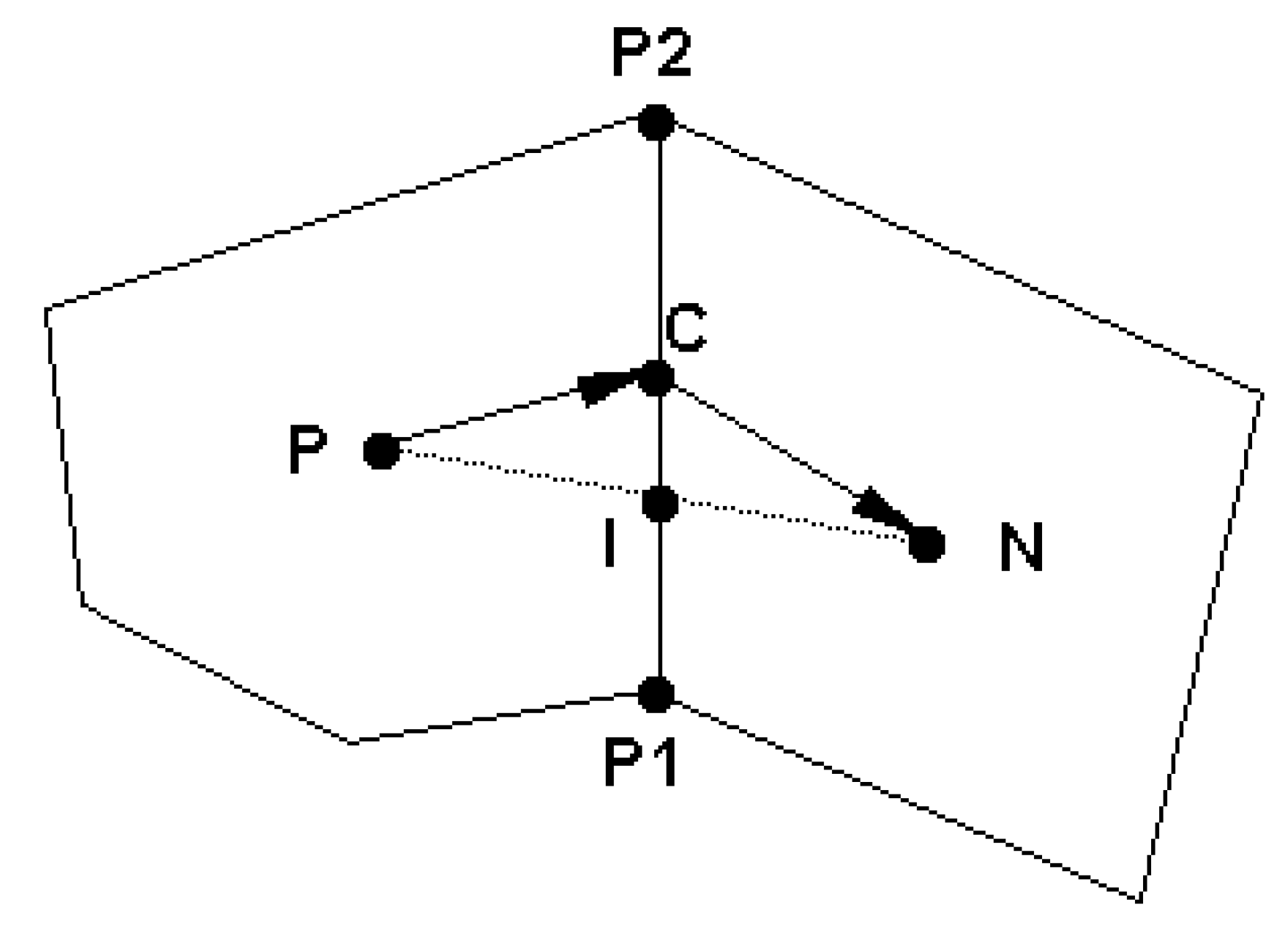
Here denotes a sediment dependent variable, is the diffusivity, and is the source/sink term. Integration over an arbitrarily shaped polygon P shown in Figure 1. leads to:
In the above, is time step, A is polygon area, is the velocity component normal to the polygon side (e.g., P1P2 in Figure 1) and evaluated at the side center C, is polygon side unit normal vector, is the polygon side distance vector (e.g., from P1 to P2 in Figure 1), and .
Subscript C indicates a value evaluated at the center of a polygon side and superscript, n or n + 1, denotes the time level. In the remaining discussion, superscript n + 1 will be dropped for ease of notation. Note that the first-order Euler implicit time discretization is adopted. The main task of the discretization is to obtain appropriate expressions for the convective and diffusive fluxes at each polygon side.
Discretization of the diffusion term, the first on the right-hand side of Equation (23), needs further attention. The final expression for can be written as:
In the above, is the distance vector from P to C and is from C to N. The normal and cross diffusion coefficients, and , at each polygon side involve only geometric variables; they are calculated only once in the beginning of the computation.
Calculation of a variable, say Y, at the center C of a polygon side is discussed next. This is an interpolation operation used frequently for variables. A second-order accurate expression is derived below. As shown in Figure 1, a point I is defined as the intercept point between line PN and line P1P2. A second-order interpolation for point I may be derived to be:
With and . may be used to approximate the value at the side center C. This treatment, however, does not guarantee second-order accuracy unless and are parallel. A truly second-order expression is derived to be:
in the convective term of Equation (23) adopts the second-order scheme with a damping term. It is derived by blending the first-order upwind scheme with the second-order central difference scheme and may be expressed as:
In the above, is the second-order interpolation scheme, and d defines the amount of damping used. In most applications, d = 0.2 ~ 0.3 may be used.
With expressions for the diffusion and convection terms done, the final discretized governing equation at the cell P may be organized as the following linear equation:
where “nb” refers to all neighboring polygons surrounding polygon P. The coefficients in this equation are:
Other sediment equations such as the bed elevation equation and the bed dynamics equations may be discretized similarly. In terms of time integration, the fraction step method of Yanenko [51] is used. The procedure is as follows:
The advection Equation (30a) is solved implicitly to obtain an intermediate solution with known values at time level n; the initial value problem of (30b) is solved analytically to obtain the new solution at time level (n + 1). The solutions of the bed elevation equation and bed dynamics equations are relatively straightforward and details are not presented.
4. Model Verification and Validation
Five cases are selected to verify and validate the new sediment transport mobile-bed model and results are described below. The flow module has been verified and validated before [32]; only sediment cases are presented.
4.1. Aggradation in a Straight Channel
Aggradation in alluvial streams may occur due to a variety of reasons. A common scenario is the oversupply of incoming sediments above the stream transport capacity. This may happen in the field after, e.g., heavy precipitation in a large tributary area. The case of the flume experiment of Soni [52] is selected to verify the aggradation simulation capability with the new model.
The case consists of a flat plate bed with a length of 30 m, width of 0.2 m, and slope of 0.00427. The bed is covered with sands with a medium diameter (d50) of 0.32 mm, sand depth of 0.15 m, and specific gravity of 2.65. The case has a constant flow unit discharge of 0.0355 m2/s, average velocity of 0.493 m/s, and average water depth of 0.072 m. Equilibrium of flow and sediment transport is established first by simulating long enough in time so that the upstream equilibrium sediment rate is balanced by the transport capability. Excessive sediment is then added suddenly from the upstream. The Manning’s roughness coefficient is 0.02294 in order to establish the flow equilibrium given the bed slope and flow velocity. Aggradation process is initiated immediately after a sudden increase of the sediment supply rate above the capacity. The excess sediment supply is with the sediment transport capacity. Bedload transport mode was observed in the flume experiment and is used for the simulation.
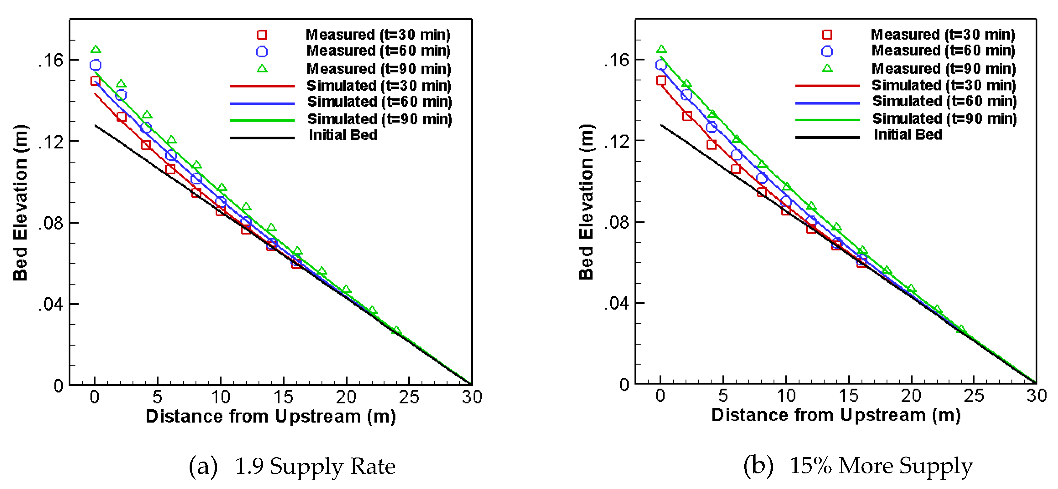
A 30-by-5 mesh is used, covering the 30 m by 0.2 m flume bed. The flow is 1D in nature so the number of cells in the lateral direction is not important. The time step used is 1.0 s. Further refinement of the mesh or reduction in time step does not change the results more than a few percentages. The simulation is first carried out for 100 min using the upstream sediment supply being ; this way the equilibrium flow and sediment transport is established (no net sediment exchanges between water column and bed). Aggradation simulation then starts with 1.9 times the sediment capacity.
A comparison of the simulated and measured bed elevation changes in time is shown in Figure 2a. Overall agreement is fair, but the model under-predicts the aggradation at a late time (e.g., at 90 min). This may be due to the high uncertainty of the measured data. Soni [52] reported that up to 15% of errors existed in the rate of sediment addition at the upstream. Another run is made by using a higher sediment supply rate to check the model sensitivity to the supply rate. The rate is increased by 15% and the results are recomputed as shown in Figure 2b. A much better agreement is obtained. In the present modeling the Engelund-Hansen capacity equation is adopted.
4.2. Erosion in a Straight Channel
Channel erosion and bed armoring occur in many situations such as downstream of a dam. They represent an important class of alluvial processes. Herein the flume experiment of Ashida and Michiue [53] is selected to verify the erosion modeling capability of the new model.
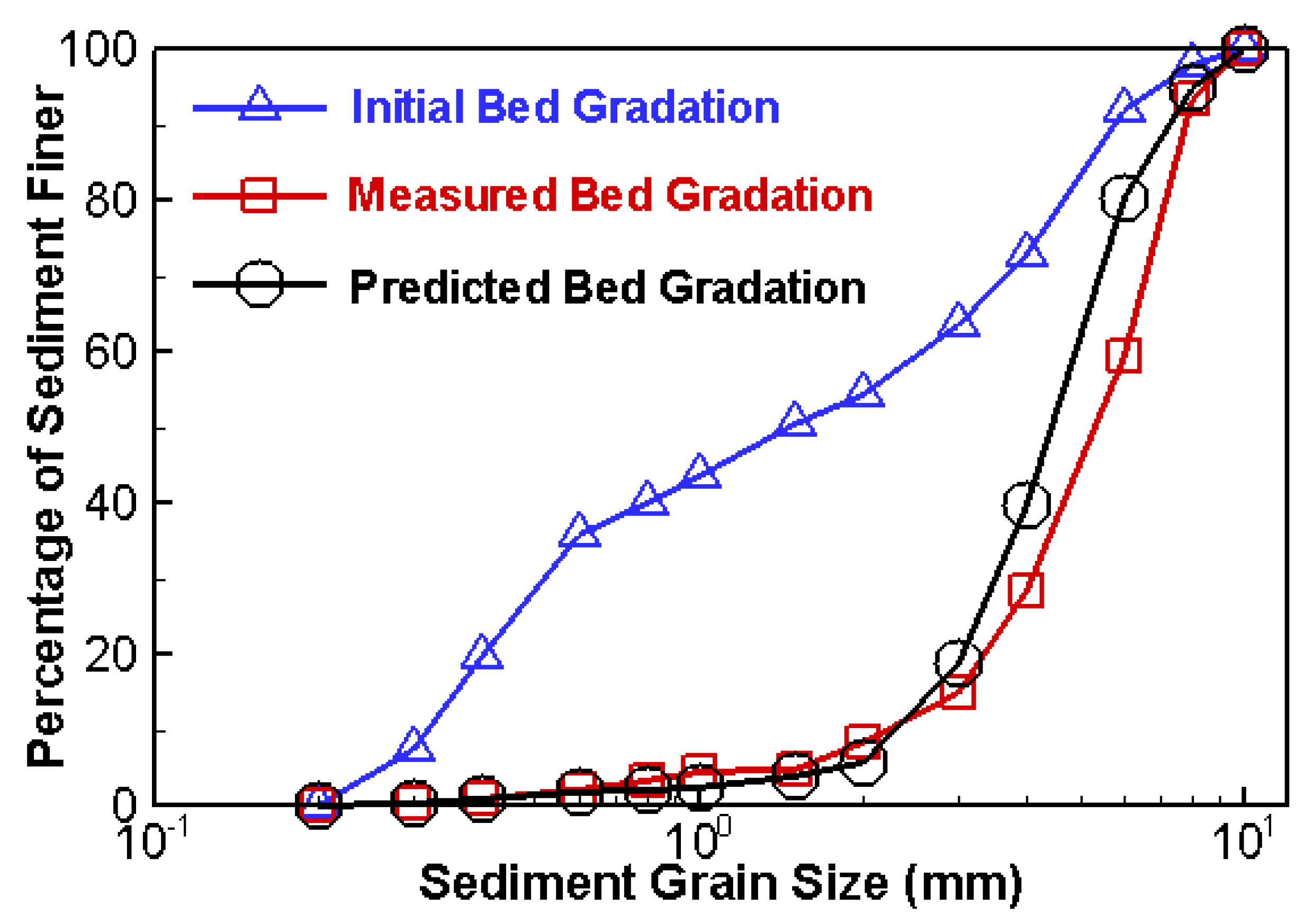
The flume used in the experiment was rectangular; it had the width of 0.8 m, length of 20 m, and bed slope of 0.01. The flume bed was filled with non-uniform sediments—a mixture of sands and fine gravels ranging from 0.2 to 10.0 mm in size. The sediment mixture had a medium diameter of 1.5 mm and a standard deviation of 3.47 (Figure 3 shows the initial bed gradation). The simulated case has a constant clear water flow of 0.0314 m3/s, an average velocity of 0.654 m/s, and water depth of 6.0 mm at the downstream boundary.
A 42-by-6 mesh is used for the simulation, covering the 20 m by 0.8 m model domain (channel bed). Note that the lateral mesh number is not important due to the 1D nature of the flow. The time step is 1.0 second. Further refinement of the mesh in the flow direction or reduction of the time step does not change the solutions more than a few percentages. Twelve sediment size classes are used to represent the sediment mixture. The range of size classes and the corresponding initial fractional gradations on the bed are in Table 1; the initial bed gradation is also plotted in Figure 3. The Manning’s roughness coefficient is 0.025; it is based on the flow calibration to achieve flow equilibrium with the given slope and velocity. For a mixed sand-gravel bed, the Parker sediment capacity equation is used with the default constants (i.e., and ). At time zero, clear water flows into the channel; afterwards, the degradation process is initiated. Only bedload transport was observed in the experiment and is thus simulated.
The experimental data showed that erosion started immediately once flow enters the flume and scour depth increased quickly for the first 100 min. Afterwards, erosion slowed down and an armoring layer was formed. The model-predicted, armored bed gradation is shown in Figure 3 at a location of 10 m from the downstream boundary. A comparison with the measured gradation at the same location shows that the agreement is relatively good, indicating the ability of the new model to predict the armoring process.
The erosion process is also compared between the model and the flume data in Figure 4 at three locations. The prediction of the time-varying scour process is less satisfactory, but the final maximum scour is predicted well. In view of a better prediction reported by Wu [16], we had tried to find out the cause. According to the discussion in [16], along with a personal communication with Dr. Wu, the cause was attributed to the bedform change while the scour was developing: the bedform was changing from a flat bed to a fully developed bed in the flume experiment. In the modeling of Wu [16], the bedform change was taken into account by adopting a time-dependent variation of the bed grain shear stress. The present modeling, however, used a constant. In order to see the impact of the time-varying bedform, the same functional form of the grain shear stress used by [16] is implemented; the model is run again without changing other model inputs. The new predicted scour results are shown in Figure 4 as dashed lines, designated as “Predicted: Wu Grain Stress.” It is seen that the variable grain stress procedure indeed improves the agreement between the model prediction and measured data, and the new results are close to Wu [16]. Since the grain stress changing procedure used is not general; it is not implemented as a feature in the new model. We prefer to take the results without the treatment (in solid lines) as the model prediction. The study, however, points to potential uncertainty in model predictions when bedform changes. Future studies are needed on how to incorporate a more general procedure so that bedform changes may be taken into accounts.
4.3. Erosion and Depostion in Bends
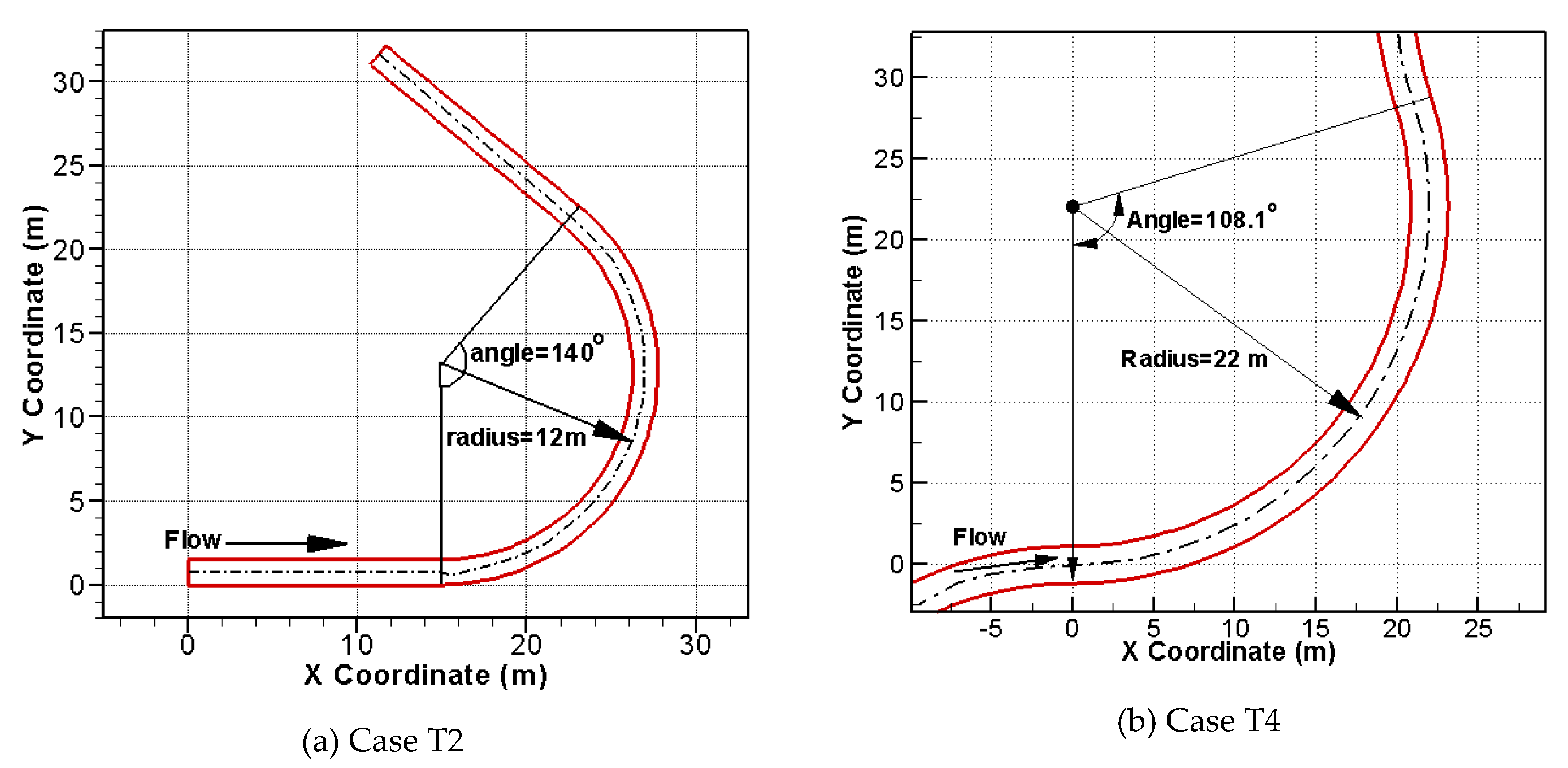
Two bend flows, reported by Struiksma et al. [54], are used to validate the ability of the new model to simulate erosion and deposition in stram bends. One is case T2 with a 140° bend filled with uniform sediments; the other is case T4 with a 108.1° bend filled with non-uniform sediments. The geometry of the two bends is shown in Figure 5. Both were tested at the Delft Hydraulics Laboratory: T2 used the DHL curved flume and T4 used the Waal Bend flume.
Case T2 had a length of 29.32 m and a radius of curvature of 12 m (Figure 5); relevant geometry and test conditions are listed in Table 2. The flume bed was initially flat laterally and filled with uniform sediments of 0.45 mm in diameter. The equilibrium bed topography was achieved after long enough water flow over the flume bed.
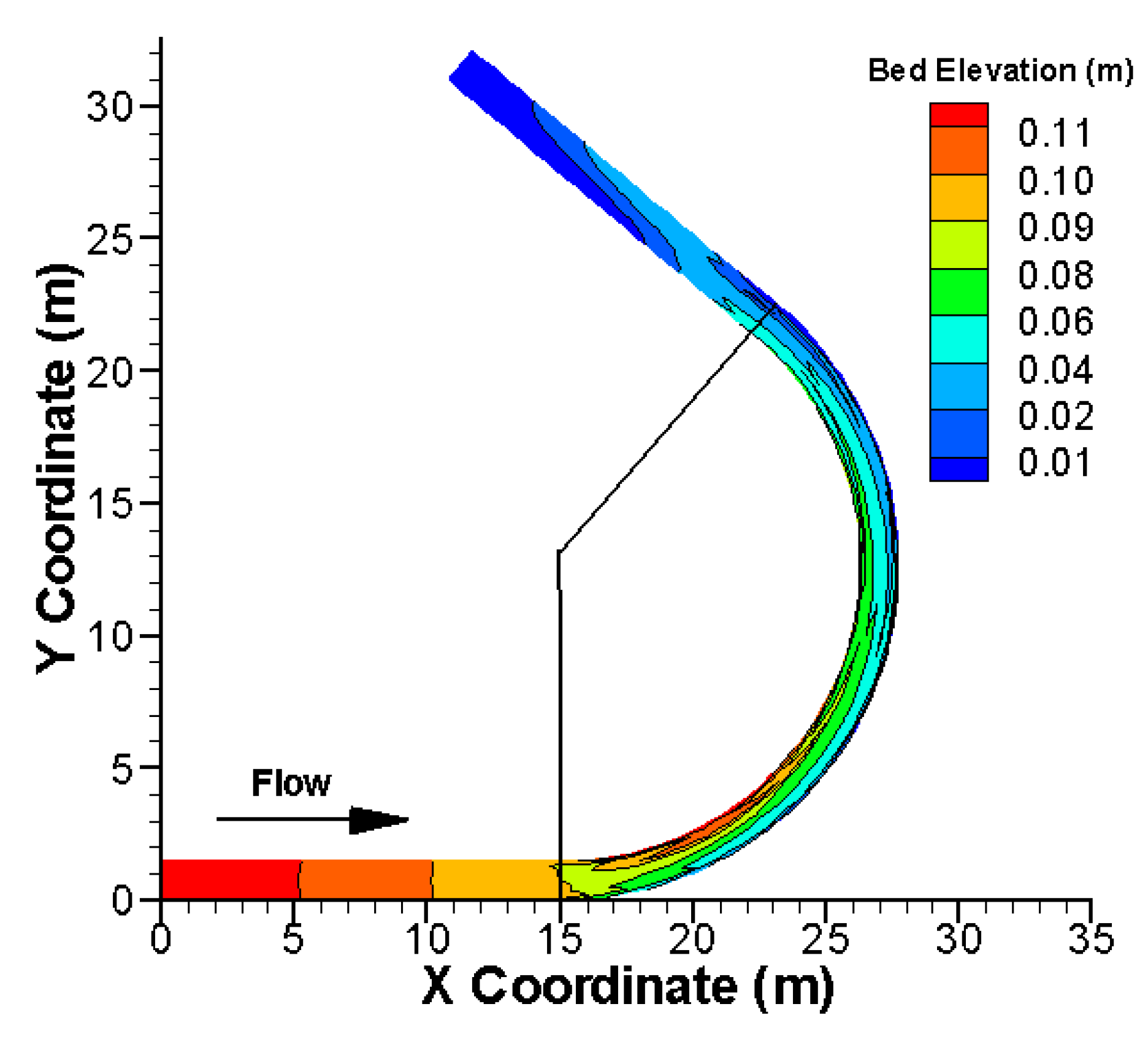
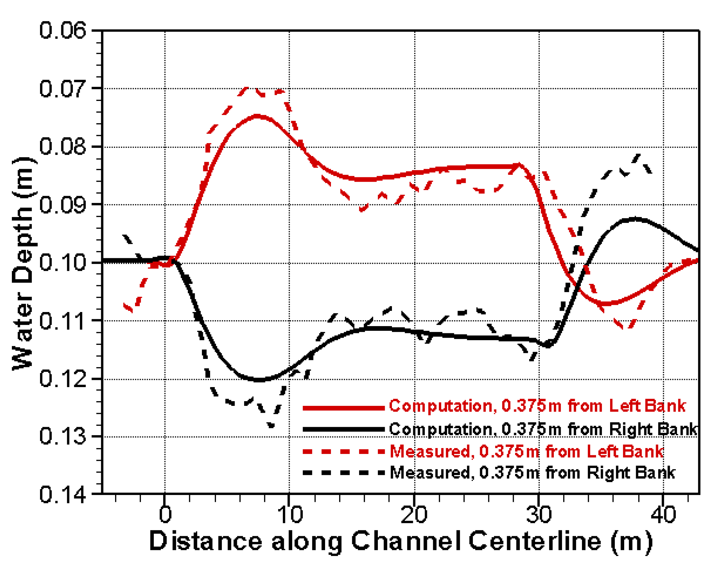
A total of 960 mesh cells are used to cover the mode domain. Further mesh refinement has not changed the results more than 2%. An unsteady simulation is carried out with a time step of 10 seconds. At the upstream (x = 0), a flow discharge of 0.062 m3/s is imposed, and the sediment supply rate is estimated with the sediment capacity equation. At the exit, the water surface elevation of 0.1 m is maintained. The Engelund-Hansen sediment capacity equation is used and the beadload transport mode is adopted based on the laboratory observation. The equilibrium bedform is reached after a sufficient time (about 10 hours) and the computed bed elevation is shown in Figure 6. In addition, a comparison of the computed and measured water depths along two profiles, 0.375 m from the inner and the outer banks, is shown in Figure 7.
The comparisons show that the new model predicts the pool and bar formation adequately although the initial bed is flat laterally. A bar is formed at the inner bank while a pool occurs at the outer bank. The agreement between the computation and measurements is satisfactory.
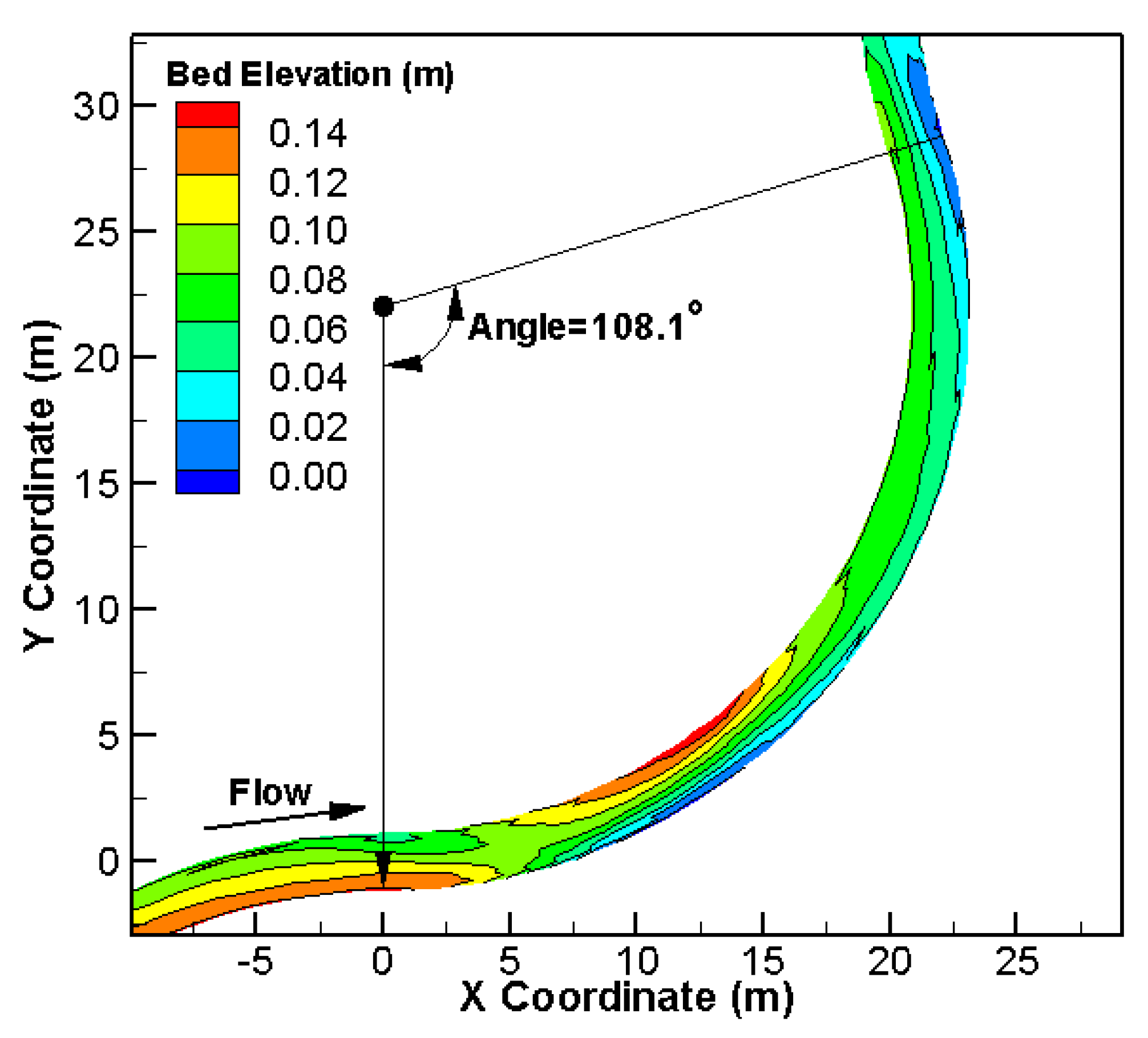
Next, case T4 is simulated: it consisted of a bend with a circular arc of 108.1o turn and 41.5 m in length. Both the entrance and exit of the bend have a section of the straight channel attached. The radius of the arc from the centerline was 22 m. Initial bed had a slope of 0.128% longitudinally but flat laterally. The bed was covered with non-uniform mixtures having mm. Some characteristic parameters of the case are listed in Table 3.
The 2D mesh consists of 1824 cells which is found sufficient as further refinement has not changed the results more than a few percentages. The sediment mixture is divided into four size classes: 15.9% of fine sand (0.125 to 0.26 mm), 34.1% medium sand (0.26 to 0.6 mm), 34.1% coarse sand (0.6 to 1.38 mm), and 15.9% vary coarse sand (1.38 to 2.0 mm). A truly unsteady simulation is carried out with a time step of 10 seconds. The bed is initially filled with the sediment mixture. At the upstream (x = 0), a flow discharge of 0.121 m3/s is imposed and the sediment supply is calculated with the sediment capacity equation. At the exit, the water surface elevation is maintained at 0.12 m.
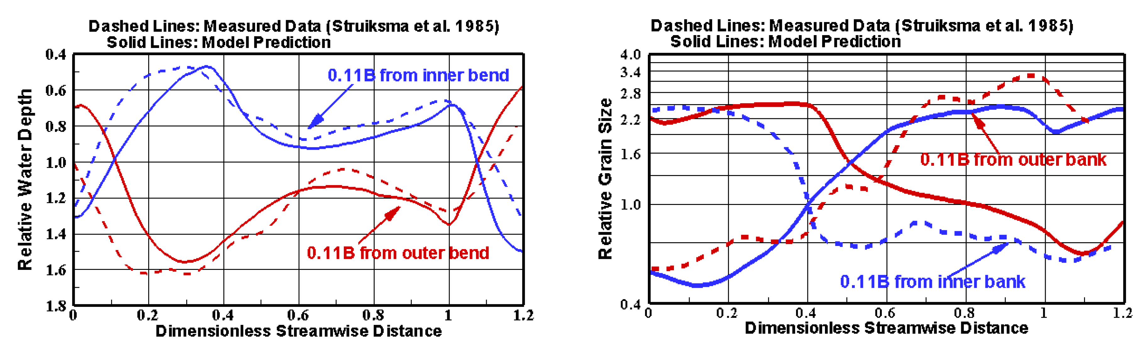
The equilibrium bedform is obtained after about 10 hours and plotted in Figure 8. A comparison of the computed and measured equilibrium water depth and medium sediment diameter () is shown in Figure 9 along two profiles: 0.11B from the inner and outer banks (B = 2.3 m is the channel width). A comparison with the measured data shows that the new model is capable of predicting the pool and bar formation as well as the sediment sorting process. Overall agreement between the model and measured data is good.
4.4. Alternating Bar Formation Downstream of an Inserted Dike
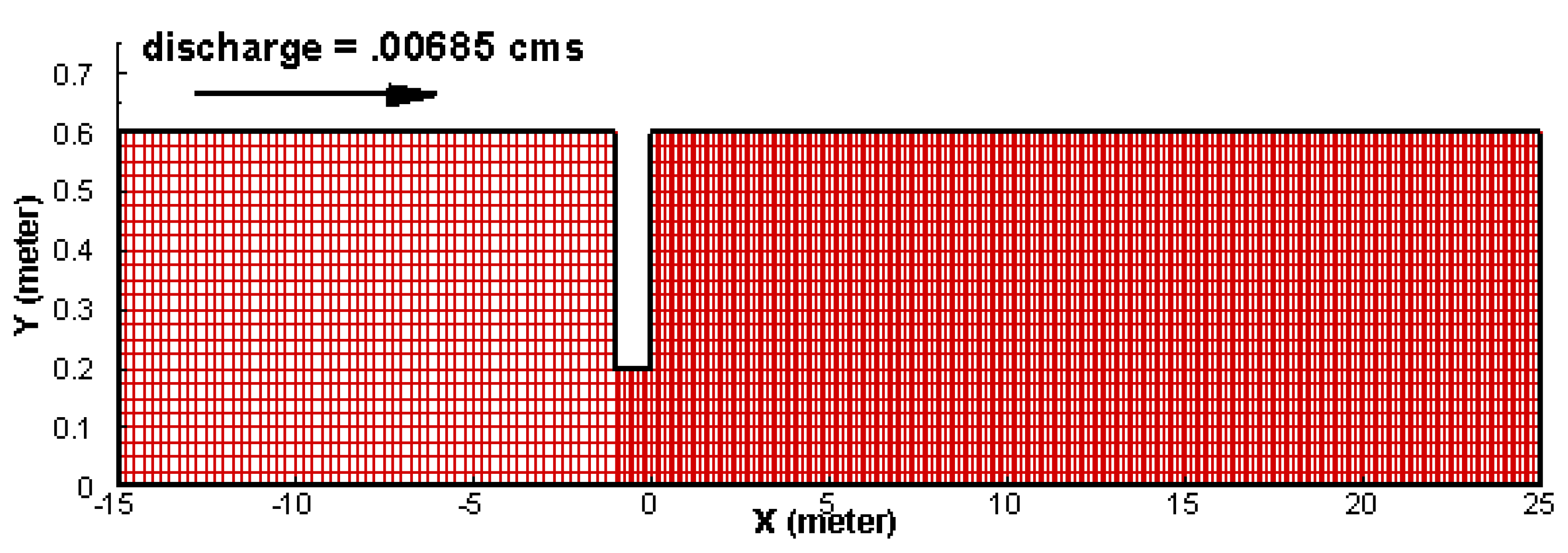
Alternate bar formation study was carried out at the Delft Hydraulics Laboratory by Struiksma and Crosato [35]. When a dike was inserted into a straight channel, forced alternate bars were formed downstream. The flume experiment started with a straight channel 0.6 m in width and 0.3% in slope under a well-defined constant flow. At the upstream, a plate (dike) was inserted to restrict the inflow section. The channel bed was initially flat and covered with almost uniform fine sediments with a median diameter (d50) of 0.216 mm. When the bed reached equilibrium, bed topography was measured which is available for numerical model verification. The experimental conditions are shown in Table 4.
The numerical model domain and the mesh are shown in Figure 10. The mesh consists of 236-by-24 cells; it is sufficient as a further refinement has not changed the results by more than a few percentages. An unsteady simulation is carried out, with a time step of 5 seconds, until equilibrium bed topography is reached. At the upstream (x = −15.0 m), a constant discharge of 0.00685 m3/s is imposed and the sediment supply rate is based on the sediment transport capacity as equilibrium solution is sought. At the downstream (x = 25 m), a water depth of 0.044 m is specified. The Parker capacity equation is used.
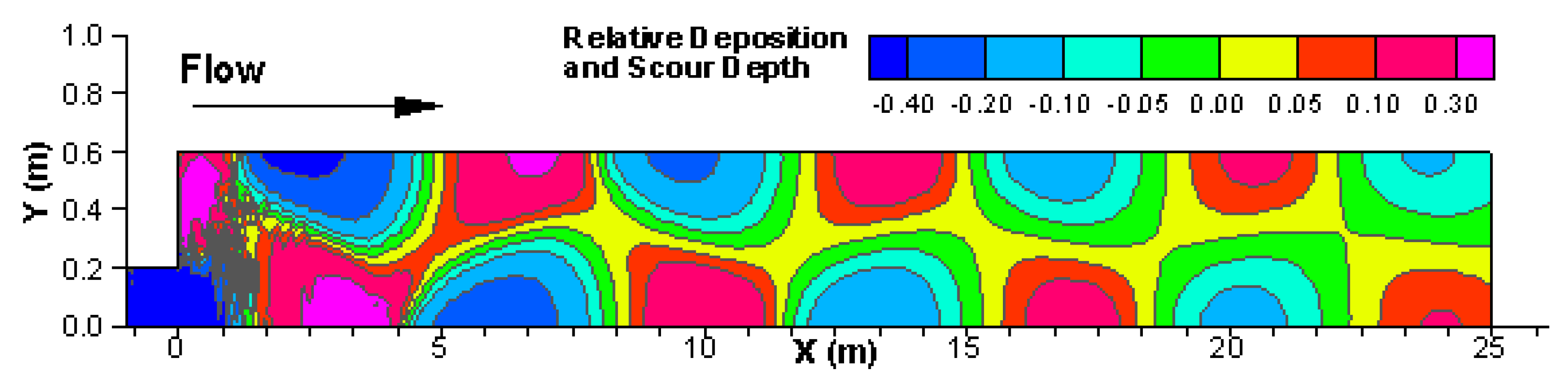
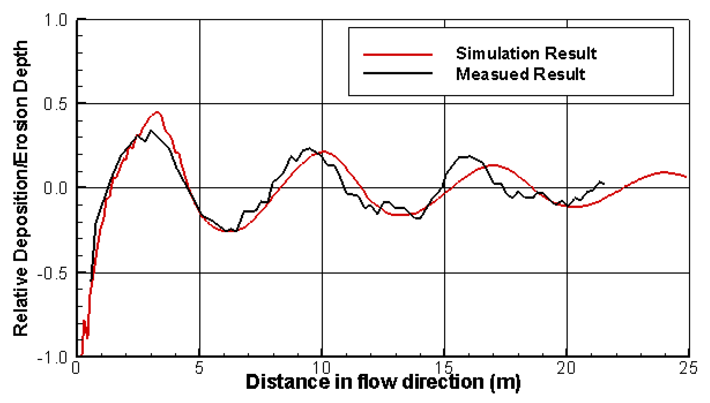
The predicted equilibrium bed topography, in the form of net erosion and deposition, is displayed in Figure 11; a comparison of the equilibrium bed profile between the model and measured data is in Figure 12 along a line 0.1 m from the bottom boundary. It is seen that a series of alternating bars are developed downstream of the dike. The bar and pool depths (amplitude) are, on average, about 25% of the average water depth, and the amplitude is mildly damped downstream. The average bar wavelength is approximately eleven times the channel width, much larger than the typical downstream migrating free bars. Results in Figure 12 show that the comparison between the prediction and measured data is good. The amplitude of the alternate bars is predicted satisfactorily while the wavelength is slightly over-predicted. The results demonstrate that the fully non-linear numerical models such as the present model is capable of predicting the alternate bar development as a response to disturbances introduced into a stream.
4.5. Erosion and Deposition on a Section of the Middle Rio Grande
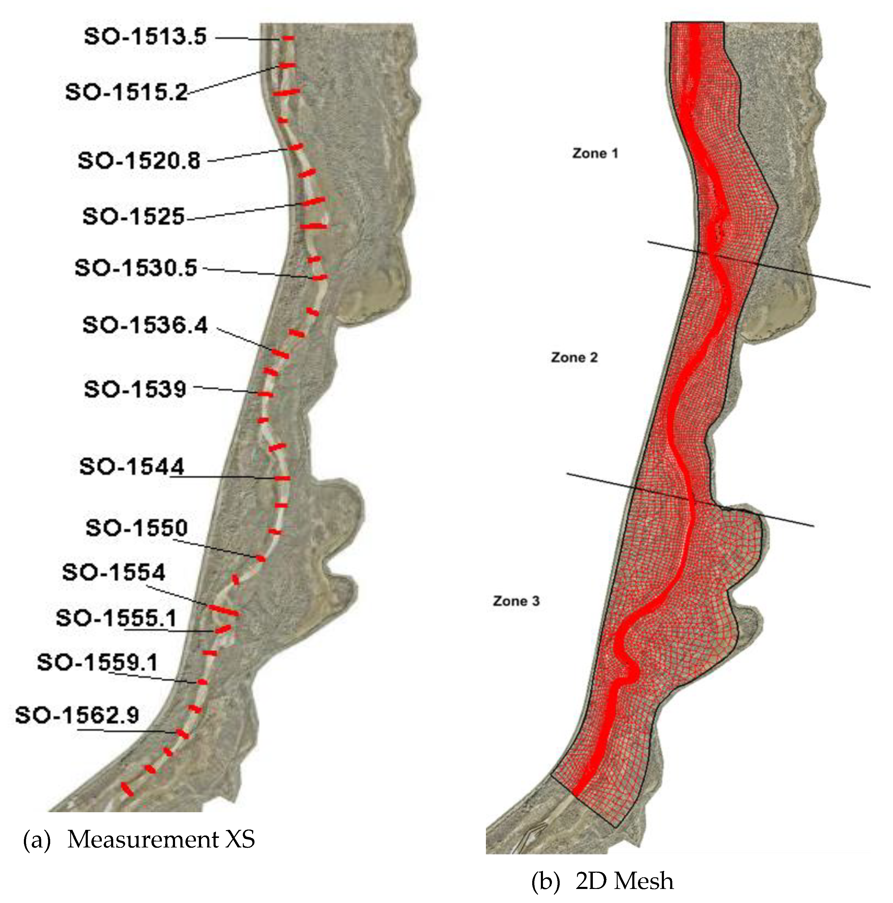
Finally, the new model is applied to a section of the Middle Rio Grande (MRG) for validation and application—the Bosque del Apache National Wildlife Refuge (BDANWR) area. BDANWR is about 11 miles upstream of the Tiffany Junction. In May 2008, BDANWR experienced a plug formation—a sudden and large sediment deposition which blocked the flows in the main river. This section has been subject to extensive field studies since to understand the erosion and deposition processes after a pilot channel was dug to reconnect the main river [55,56]. Measured bed elevation changes on many cross-sections (Figure 13a) were available in both 2008 and 2009 so modeling results may be compared and validated.
The simulated MRG section has the upstream at the North Boundary of BDANWR near SO-1513.5 (river mile 84) and the downstream boundary near SO-1564.4 (river mile 78.7)—see Figure 13a for the locations. The solution domain covers about 5.3 miles longitudinally. The 2D mesh consists of mixed quadrilaterals and triangles with a total of 10,865 cells (Figure 13b).
Other model inputs are as follows. The Manning’s roughness coefficient is based on the 1D modeling studies by Borough [57] and Collin [58] without changes. Bed sediment gradation prior to the plug formation is based on the data collected by Bauer [59] in June and July 2006. The data showed that about 99.5% of the sediments ranged from 0.0625 to 16 mm in diameter with = 0.33 mm. In the numerical modeling, seven size classes are used to represent all sediments (0.0625–16 mm) in the system. An unsteady simulation is carried out for the time period from the beginning of November 2008 to the end of July 2009. The flow discharge at the upstream is based on the daily mean flow measured at the USGS San Acacia station (#08354900), while the sediment input is based on the rating curve developed by Collins [58]. The Engelund-Hansen equation is used for the sediment capacity.
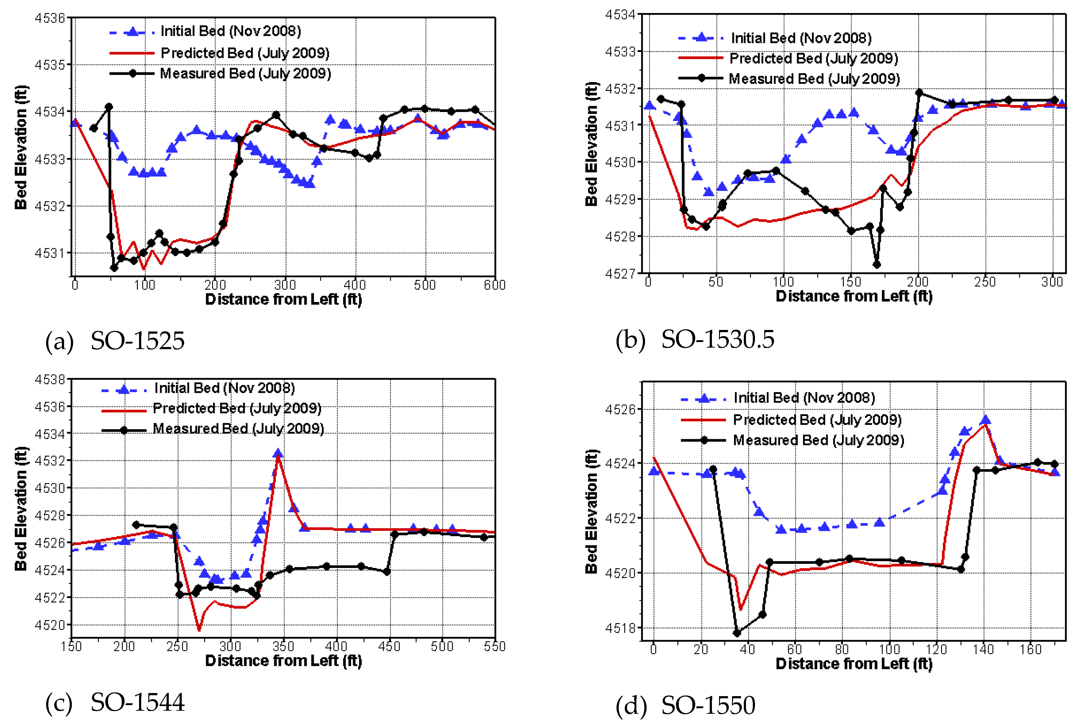
The erosion and deposition of the study reach in the period of 1 November 2008 to 31 July 2009 are simulated with the new model. The predicted channel bed elevation changes are compared with the cross-section data measured in July 2009. Comparisons at four cross sections are displayed in Figure 14. Overall, the reach is mostly erosional during the simulation period, which is expected as the plug formed in May 20018 was being eroded after the pilot channel was dug in October 2008. The agreement between the predicted and measured erosion is relatively good except for a small section between SO-1539 and SO-1544. At SO-1544, e.g., incising is predicted, not widening. This is due to that the new model does not simulate bank erosion so channel widening is not predicted.
5. Conclusions
A new depth-averaged 2D sediment transport mobile-bed model is developed, verified and validated. New contributions of the proposed model include: (a) polygon-based mesh; (b) a single sediment transport equation simulating suspended load, bedload and mixed load simultaneously; (c) truly unsteady, tightly-coupled modeling among flow, sediment transport and bed dynamics modules; and (d) a generally applicable formulation for multi-size, non-equilibrium sediment transport. The model is named SRH-2D and has been freely released to the public.
There are other features of the new model. For example, multiple subsurface bed layers are allowed so that bed stratigraphy may be taken into consideration in erosion simulation. The finite-volume method is adopted such that mass conservations of both water and sediment are satisfied locally and globally. Implicit time integration is used so that the solution process is robust and stable.
In this paper, four flume cases are selected to verify the new model, and the erosion and deposition of a section of the Middle Rio Grande is used as a validation and demonstration case. Model results have been compared with the available measured data. It is found that the agreement has been good for all cases.
Funding
The research was funded by the Science and Technology Office, U.S. Bureau of Reclamation and the Water Resources Agency, Taiwan.
Conflicts of Interest
The authors declare no conflict of interest.
References
- ASCE. Earthen embankment breaching. J. Hydraul. Eng. 2011, 137, 1549–1564. [Google Scholar] [CrossRef]
- Gibson, S.; Brunner, G.; Piper, S.; Jensen, M. Sediment Transport Computations in HEC-RAS. In Proceedings of the Eighth Federal Interagency Sedimentation Conference (8th FISC), Reno, NV, USA, 2–6 April 2006; pp. 57–64. [Google Scholar]
- USACE. New One-Dimensional Sediment Features in HEC-RAS 5.0 and 5.1. 2018. Available online: https://www.researchgate.net/publication/317073446_New_One-imensional_Sediment_Features_in_HEC-RAS_50_and_51 (accessed on 10 January 2020).
- DHI. MIKE 11. In Users Manual; Danish Hydraulic Institute: Horsholm, Denmark, 2005. [Google Scholar]
- Wu, W.; Vieira, D.A. One-Dimensional Channel Network Model CCHE1D Version 3.0.—Technical Manual; Technical Report No. NCCHE-TR-2002-1; National Center for Computational Hydroscience and Engineering, The University of Mississippi: Oxford, MS, USA, 2002. [Google Scholar]
- Huang, J.; Greimann, B.P. GSTAR-1D, General Sediment Transport for Alluvial Rivers—One Dimension; Technical Service Center, U.S. Bureau of Reclamation: Denver, CO, USA, 2007. [Google Scholar]
- FHWA. Evaluating Scour at Bridges, HEC-18, 5th ed.; Report, No. HIF-FHWA-12-003; Arneson, L.A., Zevenbergen, L.W., Lagasse, P.F., Clopper, P.E., Eds.; U.S. Department of Transportation, Federal Highway Administration: Washington, DC, USA, 2012.
- Hogan, S.A. Advancements in Bridge Scour Assessment with 2D Hydraulic Modeling Using SRH-2D/SMS. In Proceedings of the 9th International Conference on Scour and Erosion, Taipei, Taiwan, 5–8 November 2018. [Google Scholar]
- Chow, V.T.; Ben-Zvi, A. Hydrodynamic modeling of two-dimensional watershed flow. J. Hydraul. Div. ASCE 1973, 99, 2023–2040. [Google Scholar]
- Kuipers, J.; Vreugdenhil, C.B. Calculation of Two Dimensional Horizontal Flow; Reports S163, Part 1; Deflt Hydraulics Lab.: Delft, The Netherlands, 1973. [Google Scholar]
- Celik, I.; Rodi, W. Modeling suspended sediment transport in nonequilibrium situations. J. Hydraul. Eng. 1998, 114, 1157–1191. [Google Scholar] [CrossRef]
- Spasojevic, M.; Holly, F.M., Jr. 2-D bed evolution in natural watercourses—New simulation approach. J. Waterw. Port Coast. Ocean Eng. 1990, 116, 425–443. [Google Scholar] [CrossRef]
- Minh Duc, B. Berechnung der Stroemung und des Sedimenttransorts in Fluessen Mit Einem Tieffengemittelten Numerischen Verfahren. Ph.D. Thesis, The University of Karlsruhe, Karlsruhe, Germany, 1998. (In German). [Google Scholar]
- Olsen, N.R.B. Two-dimensional numerical modeling of flushing processes in water reservoirs. J. Hydraul. Res. 1999, 37, 3–16. [Google Scholar] [CrossRef]
- Wu, W.; Wang, S.S.Y.; Jia, T.; Robinson, K.M. Numerical simulation of two-dimensional headcut migration. In Proceedings of the 1999 International Water Resources Engineering Conference, on CD-ROM., ASCE, Seattle, WA, USA, 8–12 August 1999. [Google Scholar]
- Wu, W. Depth-averaged two-dimensional numerical modeling of unsteady flow and non-uniform sediment transport in open channels. J. Hydraul. Eng. 2004, 130, 1013–1024. [Google Scholar] [CrossRef]
- Hung, M.C.; Hsieh, T.Y.; Wu, C.H.; Yang, J.C. Two-dimensional nonequilibrium noncohesive and cohesive sediment transport model. J. Hydraul. Eng. 2009, 135, 369–382. [Google Scholar] [CrossRef] [Green Version]
- Huang, W.; Cao, Z.; Pender, G.; Liu, Q.; Carling, P. Coupled flood and sediment transport modelling with adaptive mesh refinement. Sci. China Technol. Sci. 2015, 58, 1425–1438. [Google Scholar] [CrossRef]
- Jia, Y.; Wang, S.S.Y. CCHE2D: Two-Dimensional Hydrodynamic and Sediment Transport Model for Unsteady Open Channel Flows Over Loose Bed; Technical Report: NCCHETR-2001-01; National Center for Computational Hydroscience and Engineering, The University of Mississippi: Oxford, MS, USA, 2001. [Google Scholar]
- Hervouet, J.-M. Hydrodynamics of Free Surface Flows; John Wiley & Sons, Ltd.: Hoboken, NJ, USA, 2007; pp. 1–360. [Google Scholar]
- Casulli, V.; Walters, R.A. An unstructured grid, three dimensional model based on the shallow water equations. Int. J. Numer. Methods Fluids 2000, 32, 331–348. [Google Scholar] [CrossRef]
- Bever, A.J.; MacWilliams, M.L. Simulating sediment transport processes in San Pablo Bay using coupled hydrodynamic, wave, and sediment transport models. Mar. Geol. 2013, 345, 235–253. [Google Scholar] [CrossRef]
- Deltares. Delft3D-FLOW. In Simulation of Multi-Dimensional Hydrodynamic Flow and Transport Phenomena, including Sediments–User Manual; Version 3.04, rev. 11114; Deltares: Delft, The Netherlands, 2010. [Google Scholar]
- Kernkamp, H.W.J.; Van Dam, A.; Stelling, G.S.; De Goede, E.D. Efficient scheme for the shallow water equations on unstructured grids with application to the Continental Shelf. Ocean Dynam. 2010, 29, 1175–1188. [Google Scholar] [CrossRef]
- Achete, F.M.; van der Wegen, M.; Roelvink, D.; Jaffe, B. A 2-D process-based model for suspended sediment dynamics: A first step towards ecological modeling. Hydrol. Earth Syst. Sci. 2015, 19, 2837–2857. [Google Scholar] [CrossRef] [Green Version]
- Deltares. D-Flow Flexible Mesh, Technical Reference Manual; Deltares: Delft, The Netherlands, 2014; 82p. [Google Scholar]
- Iverson, R.M.; Ouyang, C. Entrainment of bed material by earth-surface mass flows: Review and reformulation of depth-integrated theory. Rev. Geophys. 2015, 53, 27–58. [Google Scholar] [CrossRef]
- Cao, Z.; Xia, C.; Pender, G.; Liu, Q. Shallow water hydro-sediment-morphodynamic equations for fluvial processes. J. Hydraul. Eng. 2017, 143, 02517001. [Google Scholar] [CrossRef]
- Liu, X.; Infante Sedano, J.A.; Mohammadian, A. A coupled two-dimensional numerical model for rapidly varying flow, sediment transport and bed morphology. J. Hydraul. Res. 2015, 53, 609–621. [Google Scholar] [CrossRef]
- Greimann, B.P.; Lai, Y.G.; Huang, J.C. Two-dimensional total sediment load model equations. J. Hydraul. Eng. 2008, 134, 1142–1146. [Google Scholar] [CrossRef]
- Lai, Y.G. Modeling Stream Bank Erosion: Performance for Practical Streams and Future Needs. Water 2017, 9, 950. [Google Scholar] [CrossRef] [Green Version]
- Lai, Y.G. Two-Dimensional Depth-Averaged Flow Modeling with an Unstructured Hybrid Mesh. J. Hydraul. Eng. 2010, 136, 12–23. [Google Scholar] [CrossRef] [Green Version]
- Rodi, W. Turbulence Models and Their Application in Hydraulics, 3rd ed.; IAHR Monograph: Rotterdam, The Netherlands, 1993. [Google Scholar]
- Odgaard, A.J. Transverse bed slope in alluvial channel beds. J. Hydraul. Div. ASCE 1981, 107, 1677–1694. [Google Scholar]
- Struiksma, N.; Crosato, A. Analysis of a 2D bed topography model for rivers. In River Meandering; Ikeda, S., Parker, G., Eds.; AGU Water Resources Monograph 12: Washington, DC, USA, 1989. [Google Scholar]
- Talmon, A.M.; van Mierlo, M.C.L.M.; Struiksma, N. Laboratory measurements of the direction of sediment transport on transverse alluvial-bed slopes. J. Hydraul. Res. 1995, 33, 495–517. [Google Scholar] [CrossRef]
- Holly, F.M.; Rahuel, J.L. New Numerical/Physical Framework for Mobile-Bed Modeling, Part 1: Numerical and Physical Principles. J. Hydraul. Res. 1990, 28, 401–416. [Google Scholar] [CrossRef]
- Engelund, F.; Hansen, E. A Monograph on Sediment Transport in Alluvial Streams; Teknish Forlag, Technical Press: Copenhagen, Denmark, 1972. [Google Scholar]
- Parker, G. Surface-based bedload transport relation for gravel rivers. J. Hydraul. Res. 1990, 28, 417–428. [Google Scholar] [CrossRef]
- Andrews, E.D. Bed material transport in the Virgin River, Utah. Water Resour. Res. 2000, 36, 585–596. [Google Scholar] [CrossRef]
- Komar. Flow competence of the hydraulic parameters of floods. In Floods: Hydrological, Sedimentological and Geomorphological Implications; Beven, K., Carling, P., Eds.; John Wiley and Sons: Chichester, UK, 1989; pp. 107–134. [Google Scholar]
- Buffington, J.M.; Montgomery, D.R. A systematic Analysis of Eight Decades of Incipient Motion Studies, with special Reference to Gravel-Bedded Rivers. Water Resour. Res. 1997, 33, 1993–2029. [Google Scholar] [CrossRef] [Green Version]
- Wilcox, P.R.; Crowe, J.C. Surface-Based Transport Model for Mixed-Size Sediment. J. Hydraul. Eng. 2003, 129, 120–128. [Google Scholar]
- Thuc, T. Two-Dimensional Morphological Computations Near Hydraulic Structures. Ph.D. Thesis, Asian Institute of Technology, Bangkok, Thailand, 1991. [Google Scholar]
- Rahuel, J.L.; Holly, F.M.; Chollet, J.P.; Belleudy, P.J.; Yang, G. Modeling of riverbed evolution for bedload sediment mixtures. J. Hydraul. Eng. 1989, 115, 1521–1542. [Google Scholar] [CrossRef]
- Gaeuman, D.; Sklar, L.; Lai, Y.G. Flume experiments to constrain bedload adaptation length. J. Hydrol. Eng. 2014, 20, 06014007. [Google Scholar] [CrossRef]
- Philips, B.C.; Sutherland, A.J. Spatial lag effect in bed load sediment transport. J. Hydraul. Res. 1989, 27, 115–133. [Google Scholar] [CrossRef]
- Han, Q.W. A study on the non-equilibrium transportation of suspended load. In Proceedings of the 1st International Symposium on River Sedimentation, IRTCES, Beijing, China, 24–29 March 1980. [Google Scholar]
- Han, Q.W.; He, M. A mathematical model for reservoir sedimentation and fluvial processes. Int. J. Sediment Res. 1990, 5, 43–84. [Google Scholar]
- Lai, Y.G.; Weber, L.J.; Patel, V.C. Non-Hydrostatic Three-Dimensional Method for Hydraulic Flow Simulation—Part I: Formulation and Verification. J. Hydraul. Eng. ASCE 2003, 129, 196–205. [Google Scholar] [CrossRef]
- Yanenko, N.N. The Method of Fractional Steps; Springer: New York, NY, USA, 1971. [Google Scholar]
- Soni, J.P. Laboratory study of aggradation in alluvial channels. J. Hydrol. 1981, 49, 87–106. [Google Scholar] [CrossRef]
- Ashida, K.; Michiue, M. An investigation of river bed degradation downstream of a dam. In Proceedings of the 14th IAHR Congress, Paris, France, 29 August–3 September 1971; Volume 3, pp. 247–256. [Google Scholar]
- Struiksma, N.; Olsen, K.W.; Flokstra, C.; De Vriend, H.J. Bed deformation in curved alluvial channels. J. Hydraul. Res. 1985, 23, 57–79. [Google Scholar] [CrossRef]
- Tetra Tech, Inc. Sediment Transport Analysis Total Load Report, June 2008, SO-1470.5 and EB-10 Lines, Tetra Tech Project No. T22541; Albuquerque Area Office, U.S. Bureau of Reclamation: Albuquerque, NM, USA, 2008.
- Lai, Y.G.; Collins, K.L. Sediment Plug Formation on the Rio Grande: A Review of Numerical Modeling; Technical Report No. SRH-2008-06; Technical Service Center, Bureau of Reclamation: Denver, CO, USA, 2008.
- Boroughs, C.B. Sediment Plug Computer Modeling Study, Tiffany Junction Reach, Middle Rio Grande Project; Albuquerque Aera Office, U.S. Bureau of Reclamation: Albuquerque, NM, USA, 2005; 122p.
- Collins, K.L. 2006 Middle Rio Grande Maintenance Modeling: San Antonio to Elephant Butte Dam. U.S. Bureau of Reclamation; Technical Service Center, Sedimentation and River Hydraulics Group: Denver, CO, USA, 2006.
- Bauer, T.R. 2006 Bed Material Sampling on the Middle Rio Grande, NM, U.S. Bureau of Reclamation; Technical Service Center, Sedimentation and River Hydraulics Group: Denver, CO, USA, 2006.
Figure 1.
Schematic illustrating a polygon P along with one of its neighboring polygons N.

Figure 2.
Comparison of bed elevation changes in time between model prediction and flume data for the aggradation case of Soni [52]). (a) upstream, sediment rate is 1.9 the capacity; (b) upstream sediment supply is 15% more than (a).
Figure 2.
Comparison of bed elevation changes in time between model prediction and flume data for the aggradation case of Soni [52]). (a) upstream, sediment rate is 1.9 the capacity; (b) upstream sediment supply is 15% more than (a).

Figure 3.
Comparison of predicted and measured bed gradation at a location 10-m from the downstream model boundary; measured data are from Ashida-Michiue [53].
Figure 3.
Comparison of predicted and measured bed gradation at a location 10-m from the downstream model boundary; measured data are from Ashida-Michiue [53].

Figure 4.
Comparison of predicted and measured scour depth variation in time at three locations: 13 m (red), 10 m (blue), and 7 m (black) from the downstream model boundary; “Measured” = Ashida-Michiue [53]; “Wu Grain Stress” = the results obtained with the modified grain shear stress calculation.
Figure 4.
Comparison of predicted and measured scour depth variation in time at three locations: 13 m (red), 10 m (blue), and 7 m (black) from the downstream model boundary; “Measured” = Ashida-Michiue [53]; “Wu Grain Stress” = the results obtained with the modified grain shear stress calculation.

Figure 5.
Bend geometry for (a) Cases T2 and (b) Case T4 studied by Struiksma et al. [54].
Figure 5.
Bend geometry for (a) Cases T2 and (b) Case T4 studied by Struiksma et al. [54].

Figure 6.
Computed equilibrium bed elevation for case T2 of Struiksma et al. [54].
Figure 6.
Computed equilibrium bed elevation for case T2 of Struiksma et al. [54].

Figure 7.
Comparison of the computed and measured water depths along lines 0.375 m from inner and outer banks for case T2 of Struiksma et al. [54].
Figure 7.
Comparison of the computed and measured water depths along lines 0.375 m from inner and outer banks for case T2 of Struiksma et al. [54].

Figure 8.
Computed equilibrium bed elevation for case T4 of Struiksma et al. [54].
Figure 8.
Computed equilibrium bed elevation for case T4 of Struiksma et al. [54].

Figure 9.
Comparison of computed and measured water depth (left) and (right) along the lines 0.11B from the inner and outer banks for case T4 of Struiksma et al. [54].
Figure 9.
Comparison of computed and measured water depth (left) and (right) along the lines 0.11B from the inner and outer banks for case T4 of Struiksma et al. [54].

Figure 10.
Channel geometry, dimension, and 2D mesh for the Struiksma and Crosato [35] case.
Figure 10.
Channel geometry, dimension, and 2D mesh for the Struiksma and Crosato [35] case.

Figure 11.
Predicted deposit depth (positive) and erosion depth (negative).

Figure 12.
Comparison of predicted and measured erosion and deposition depths along a straight line of y = 0.1 m; depth is normalized with the average water depth of 0.044 m.
Figure 12.
Comparison of predicted and measured erosion and deposition depths along a straight line of y = 0.1 m; depth is normalized with the average water depth of 0.044 m.

Figure 13.
(a) Cross sections (XS) of the field measurement. (b) The 2D mesh for the numerical modeling (flow is from top to bottom, or North to South).
Figure 13.
(a) Cross sections (XS) of the field measurement. (b) The 2D mesh for the numerical modeling (flow is from top to bottom, or North to South).

Figure 14.
Comparison of predicted and measured bed elevation changes at four cross sections.


Table 1.
Sediment size classes and the initial fractional content (gradation) on bed.
| Diameter Range (mm) | 0.2– 0.3 | 0.3– 0.4 | 0.4– 0.6 | 0.6– 0.8 | 0.8– 1.0 | 1.0– 1.5 | 1.5– 2.0 | 2.0– 3.0 | 3.0– 4.0 | 4.0– 6.0 | 6.0– 8.0 | 8.0– 10. |
| Content (%) | 7.45 | 12.4 | 15.9 | 4.4 | 3.6 | 6.79 | 4.0 | 9.18 | 10.2 | 18.1 | 6.0 | 2.0 |
Table 2.
Flume geometry and experiment conditions for case T2 of Struiksma et al. [54].
Table 2.
Flume geometry and experiment conditions for case T2 of Struiksma et al. [54].
| Flume Width (m) | Discharge (m3/s) | Water Depth (m) | Velocity (m/s) | Bed Slope | Froude Number | d50 (mm) | Manning’s Coefficient |
|---|---|---|---|---|---|---|---|
| 1.5 | 0.062 | 0.10 | 0.41 | 0.203% | 0.41 | 0.45 | 0.023 |
Table 3.
Flume geometry and experiment conditions for case T4 of Struiksma et al. [54].
Table 3.
Flume geometry and experiment conditions for case T4 of Struiksma et al. [54].
| Flume Width (m) | Discharge (m3/s) | Water Depth (m) | Velocity (m/s) | Bed Slope | Froude Number | d50 (mm) | Manning’s Coefficient |
|---|---|---|---|---|---|---|---|
| 2.3 | 0.121 | 0.12 | 0.44 | 0.128% | 0.41 | 0.60 | 0.02 |
Table 4.
Key flume geometry and experiment conditions with the Struiksma and Crosato [35] case.
Table 4.
Key flume geometry and experiment conditions with the Struiksma and Crosato [35] case.
| Flume Width (m) | Discharge (m3/s) | Water Depth (m) | Velocity (m/s) | Bed Slope | Froude Number | Manning’s Coefficient |
|---|---|---|---|---|---|---|
| 0.60 | 0.00685 | 0.044 | 0.26 | 0.3% | 0.39 | 0.0263 |
© 2020 by the author. Licensee MDPI, Basel, Switzerland. This article is an open access article distributed under the terms and conditions of the Creative Commons Attribution (CC BY) license (http://creativecommons.org/licenses/by/4.0/).
Share and Cite
MDPI and ACS Style
Lai, Y.G. A Two-Dimensional Depth-Averaged Sediment Transport Mobile-Bed Model with Polygonal Meshes. Water 2020, 12, 1032. https://doi.org/10.3390/w12041032
AMA Style
Lai YG. A Two-Dimensional Depth-Averaged Sediment Transport Mobile-Bed Model with Polygonal Meshes. Water. 2020; 12(4):1032. https://doi.org/10.3390/w12041032
Chicago/Turabian StyleLai, Yong G. 2020. "A Two-Dimensional Depth-Averaged Sediment Transport Mobile-Bed Model with Polygonal Meshes" Water 12, no. 4: 1032. https://doi.org/10.3390/w12041032
Note that from the first issue of 2016, this journal uses article numbers instead of page numbers. See further details here.