Article

Assessing Inhomogeneities in Extreme Annual Rainfall Data Series by Multifractal Approach

by
Amanda P. García-Marín
1,*,
Javier Estévez
1,
Renato Morbidelli
2,
Carla Saltalippi
2,
José Luis Ayuso-Muñoz
1 and
Alessia Flammini
2
1
Engineering Projects Area, Department of Rural Engineering, University of Cordoba, 14071 Córdoba, Spain
2
Department of Civil and Environmental Engineering, University of Perugia, 06123 Perugia, Italy
*
Author to whom correspondence should be addressed.
Water 2020, 12(4), 1030; https://doi.org/10.3390/w12041030
Submission received: 5 March 2020 / Revised: 31 March 2020 / Accepted: 1 April 2020 / Published: 4 April 2020
(This article belongs to the Section Hydrology)

Abstract

:
Testing the homogeneity in extreme rainfall data series is an important step to be performed before applying the frequency analysis method to obtain quantile values. In this work, six homogeneity tests were applied in order to check the existence of break points in extreme annual 24-h rainfall data at eight stations located in the Umbria region (Central Italy). Two are parametric tests (the standard normal homogeneity test and Buishand test) whereas the other four are non-parametric (the Pettitt, Sequential Mann–Kendal, Mann–Whitney U, and Cumulative Sum tests). No break points were detected at four of the stations analyzed. Where inhomogeneities were found, the multifractal approach was applied in order to check if they were real or not by comparing the split and whole data series. The generalized fractal dimension functions Dq and the multifractal spectra f(α) were obtained, and their main parameters were used to decide whether or not a break point existed.

Graphical Abstract

1. Introduction

Frequency analysis of extreme rainfall data (defined as yearly maxima of a certain duration) is a common application in hydrologic engineering. It should be applied to recorded series that follow the characteristics of independency, stationarity and homogeneity [1]. Inhomogeneities in station data records can be due to observational routines (station relocations or changes in measuring techniques) and in that case, statistical methods and metadata information are effective for identifying these [2]. However, some shifts in climate dynamics are a consequence of human activities [3,4,5], or are related to El-Niño Southern Oscillation (ENSO) events such as those that occurred in 1976–77 [6], or to volcanic eruptions and changes in atmospheric composition and circulation [7].
Regardless of the reason, it is important to interpret past variability and recognize the shifts in climatic data in order to make adequate future projections. Therefore, it is crucial to investigate the effects of climate change on hydrologic time series, and especially on extreme rainfall data in order to accurately estimate or even update the intensity-duration-frequency (IDF) curves in a certain place [8]. The IDF curves are important tools for hydrologic and hydraulic design, which nowadays faces the problems of increased urbanization and population and of climate change [9], among others.
Trends in hourly, monthly, seasonal or annual rainfall series have been studied in several works with different results [10,11,12,13,14,15,16,17].
Numerous statistical methods such as the standard normal homogeneity (SNH) test, Buishand test, Pettitt test or Sequential Mann–Kendall test, among others, can be applied to evaluate the homogeneity of climate time series and have been widely used [13,18,19]. Some of the shifts detected under these classical tests turn out to be the regular behavior of time series under the scaling assumption [20,21]. Therefore, authors such as [22] recommend the consideration of scaling behavior of annual maximum rainfall when analyzing the trends in a time series, especially considering that the scaling hypothesis can increase the probability of rejection of correct null hypothesis [23]. Thus, accounting for scaling may help to avoid contradictions in trend analysis studies [23].
Authors such as [24] or [25] have analyzed changes in temporal data series during scale invariance, considering that several works have demonstrated the multifractal properties of meteorological systems [26,27,28]. Those systems exhibit the same properties for different measuring scales, thus certain behavioral information can be transferred from one scale to another, which is very useful for modeling purposes.
Sometimes, different results for the year when a shift or break point is detected in a data series are obtained by different statistical homogeneity tests, and metadata or other local and climate information cannot help to determine whether a break point really exists or not. In this work, we propose a novel use of the scale invariance properties of data sets as a useful tool to confirm whether inhomogeneities previously found in extreme rainfall data series are real or not. Moreover, the methodology can also be used to confirm the existence of a shift when only one or a few statistical tests have detected it. If a break point exists in an extreme rainfall series, the two data series derived by splitting the whole one before and after that break point should have different characteristics and can be considered as different. Therefore, the length decreases and can influence rainfall data estimation when applying frequency analysis to the two data series; this element is of great importance, especially for low return period quantile estimation, and so for IDF estimation.
For these purposes, extreme annual 24-h rainfall data from eight rain gauge stations with sufficiently long series were selected in the Umbria region (Central Italy). Six statistical homogeneity tests were applied to the selected extreme rainfall series in order to highlight inhomegeneities. The multifractal properties of the data series were then used to check the existence or not of break points detected by one or a few or all tests.

2. Materials and Methods

2.1. Data Source

Rainfall data from the Umbria region (central Italy) are used in this work. The Umbria region has an area of 8456 Km2, and is located in the Tiber river basin, which crosses the region from the north to the south-west. Its landscape is partially mountainous due to the presence of the Apennine Mountains that reach up to 2000 m a.s.l., and partially hilly in the central and western areas with altitudes ranging from 100 to 800 m a.s.l.
The mean annual rainfall for the last century is about 900 mm, with values varying in space from 650 mm to 1450 mm. The highest monthly rainfall values generally occur during the autumn–winter period, together with floods caused by widespread rainfall. The highest and lowest rainfall depths typically take place in November and July, respectively.
Five significant droughts have occurred in recent years in the region (2001 to 2003, then in 2007, 2012, 2015 and 2017) as well as six dangerous flood events (in 2005, 2008, 2010, 2012 and in 2013), with very significant economic impacts [29].
The study area is currently monitored through a dense rain gauge network (about 1 rain gauge every 90 Km2). For this study, only the stations with at least 50 continuous years of extreme 24hour duration rainfall data have been considered (Table 1): Bastia Umbra, Bevagna, Nocera Umbra, Petrelle, Ponte Nuovo di Torgiano, Spoleto, Terni and Todi. Figure 1 shows the location of the eight sites considered in the Umbria region.

2.2. Methodology

2.2.1. Homogeneity Tests

There are many statistical tests to check the homogeneity of a data series y1, y2, …, yn, with n the number of data, with specific characteristics. Some tests are known as parametric because they assume that the analyzed variable is normally distributed. Those that do not make this assumption are called non-parametric tests.
Under the null hypothesis, the annual values yi (i = 1, …, n) of the testing variable y are independent and identically distributed and the series is considered as homogeneous. Under the alternative hypothesis, the series shows a break in the mean and is considered as inhomogeneous. Moreover, there are tests that are able to give information about the year the break occurred, whereas those that assume the series is not randomly distributed under alternative hypothesis cannot provide this information.
In the present work, six homogeneity tests were applied. All of them are able to detect the year of the break if it exists. Two parametric tests were selected: the Buishand range (BR) test and the standard normal homogeneity (SNH) test. The non-parametric tests were: the Pettitt (PT) test, Tequential Mann–Kendall test (SQMK) test, Mann–Whitney U (MWU) test and Cumulative Sum (CUSUM) test.
(1)
Buishand Range test
This test is based on the adjusted partial sums or cumulative derivations from the mean of the n data points, y ¯ :
S 0 * = 0 ; S k * = i = 1 k ( y i y ¯ ) , k = 1 ,   ,   n
For a homogeneous record, S k * values fluctuate around zero. The values of S k * can be rescaled by the sample standard deviation, D y :
S k * * = S k * D y , k = 0 , ,   n
with D y 2 = i = 1 n ( y i y ¯ ) 2 n
The Q, which is sensitive to departures from homogeneity, can then be obtained as:
Q = m a x 0 k n | S k * * |
For different significance levels, the critical values for the test statistics (Qc) depend on the number of data and can be found in [30].
(2)
Standard Normal Homogeneity test
This test [31] compares the mean of the first k years of data with the last (nk) years by using the Tk of the statistics:
T k = k z 1 ¯ + ( n k ) z 2 ¯ ,     k = 1 , 2 , n
where
z 1 ¯ = 1 k   i = 1 k y i y ¯ s   , z 2 ¯ = 1 n k   i = k + 1 n y i y ¯ s   , a n d   s = 1 n   i = 1 n ( y i y ¯ ) 2
The year k shows a break if the value of Tk is the maximum. If the T 0 = max 1 k n T k is greater than the critical values [32], the null hypothesis is rejected.
(3)
Pettitt test
The Pettitt test [33] is based on the ranking ri of the yi values. The ranks ri are obtained by ordering the data in crescent order, so that the smallest one gets ranked 1 and the highest gets the n-rank. The Uk is then obtained as:
U k = 2 i = 1 k r i k ( n + 1 )       k = 1 ,   2 ,   ,   n
If a break occurs in the year K, then the Uk is:
U K = m a x 1 k n | U k |
The statistical significance of the break point is checked by comparing the value of U K (Equation (7)) to its theoretical value:
U K α = ( L n ( α ( n 3 + n 2 ) ) 6 ) 1 / 2
with α the significance level.
(4)
Sequential Mann–Kendall test
This test is usually applied to evaluate trends in data series and also to check the moment when they start being significant [34,35,36]. It calculates two series of statistic values: one (U(t)) for the progressive temporal data set (y1, y2, …, yn) and the other (U’(t)) for the corresponding regressive data set (yn, yn−1, …, y1), both with an average value of zero and a standard deviation of one. Usually, the ranks of the yi values are preferred.
The tk has to be obtained by:
t k = i = 1 k n i , ( 2 k n )
with ni being the number of cases for which y i > y j   ( j = 1 ,   2 ,   ,   i 1 ) .
Under the null hypothesis, it is assumed that no trend exists, and tk follows a normal distribution with average and variance values given by:
E [ t k ] = k ( k 1 ) 4         V a r   [ t k ] = k ( k 1 ) ( 2 k + 5 ) 72         ( 2 k n )
The sequential values of U(tk) are finally obtained as:
U ( t k ) = t k E [ t k ] V a r ( t k ) ,   ( k = 2 ,   3 ,   ,   n )
A positive value of U(tk) shows a positive trend, whereas a negative trend appears if the U(tk) value is negative.
The null hypothesis is rejected if | U ( t k ) | > Z ( 1 α 2 ) where Z ( 1 α 2 ) is the critical value of the typified normal distribution with a probability higher than α 2 . For a significance level α = 5%, the critical value of Z ( 1 α 2 ) is 1.9604.
The values of U’( t k ) are also obtained from regressive temporal data series, tk’, E[tk’], Var[tk’] by using Equations (9)–(11), and finally:
U ( t k ) = U ( t k ) w i t h   k = n + 1 j ( j = 1 ,   2 ,   ,   n )
By plotting the curves of the U(t) and U’(t) as a function of the year, a break point is detected where the curves cross and diverge.
(5)
Mann–Whitney U test
This test can detect a step change in a time series by assessing the difference in the means of two sub-series arising from splitting the complete data series. The original time series (yi, i = 1, 2, …, n) is broken into two subseries, one from y1 to yn1 and the other from yn1+1 to yn, of sizes n1 and n2 (nn1 + 1), respectively. A new data series, zt (t = 1, …, n) is obtained by rearranging the original time series yi in increasing order of magnitude. The Mann–Whitney test statistic is obtained by:
Z c = i = 1 n 1 R ( y i ) n 1 ( n 1 + n 2 + 1 ) / 2 [ n 1 n 2 ( n 1 + n 2 + 1 / 12 ] 0.5
where R(yi) is the rank of observation yi in the series zt. If | Z c | > Z ( 1 α 2 ) the hypothesis of equal means in both subseries is rejected, being Z ( 1 α 2 ) the (1 − α/2) quantile of the normal distribution.
(6)
Cumulative Sum test
The distribution-free cumulative sum technique was proposed by [37] to detect if a significant step change occurred in a given time series at a significance level α = 0.05 [38]. The null hypothesis considers that no step change exists. For the given data series yi (i = 1, …, n), the test statistics Vk is obtained as:
V k = i = 1 k s i g n   ( y i y m e d i a n )
where k = 1, 2, …, n; ymedian is the median of the time series, and the sign function is:
sign   ( y i y m e d i a n ) = { 1         i f   y i > y m e d i a n 0         i f   y i = y m e d i a n 1         i f   y i < y m e d i a n
A step-change point consists of any year when the maximal or minimal Vk falls outside the 95% confidence limit of ±1.36 n [38].

2.2.2. Multifractal Characterization

Processes that look the same regardless of the scale at which they are observed are considered to be fractal type. Natural fractal processes, such as rainfall [26] have a statistical nature and their scaling properties can be expressed by statistical relationships [39,40]. Usually, the fractal analysis of data sets is performed by means of fixed-size algorithms that rely on the subdivision of the system into smaller parts with equal size, changing that size iteratively [41].
The scaling exponents of the qth moments of the process under study can be analyzed thorough the Generalized Fractal Dimension (GFD) function, Dq, also known as the Rénji spectrum [42] by:
D q = lim r 0 log Z ( q , r ) ( q 1 ) l o g r       q 1
where Z ( q , r ) is the partition function, depending on the values of the mass distribution (μ) of the points that represent a set data composed of n data. Considering a box of length r to fill the set, the number of ni points of data included can be obtained and also the value of μ i = n i n . The partition function is then given as   Z ( q , r ) = i = 1 n μ i q . Considering the limit of Equation (16) when q→1, the value of D1 is obtained as:
D 1 = lim r 0 i = 1 n μ i l o g μ i log r
The value of Dq for q = 0 is known as the box-counting dimension or the fractal dimension of the system. For q = 1 the information entropy is obtained. The so-called correlation dimension is obtained for q = 2.
The log-log plot of Z ( q , r ) versus r gives the value of the linear segments of the mass exponent τq. The relation between the Rénji spectrum (Dq) and τq is obtained as:
τ q = ( q 1 ) D q
The Lipschitz–Hölder exponent, α q = d τ q d q , obtains the multifractal spectrum f ( α ) as:
f ( α q ) = q α q + τ q
The multifractal spectrum shows an inverted parabolic shape and its parameters can be related to interesting characteristics of the data set [25]. The smoothest and most extreme events in the process are related to the   α m a x and α m i n values, respectively. The structure of the process can be explained through the value of   α 0 . Processes with low correlation and fine structure show high values of   α 0 . Low values of α 0 are expected for regular processes. The asymmetry parameter is related to the role that extreme events play in the temporal structure of the data set. The width of the spectrum measures the degree of multifractality of the processes.

3. Results

3.1. Break Point Detection

The BR and SNH tests were applied to all the extreme annual daily rainfall data series for each station selected in the Umbria region. The results obtained for both tests are shown in Table 2, where the statistics and their critical values are given for a significance level of 0.05.
The results of the BR test show that only at the Spoleto station, the value of Q is higher than the critical one Qc, and an inhomogeneity is detected in 1977. The SNH test results show that no inhomogeneity is present in any of the data series analyzed, considering that all the statistics T0 are below their critical values T0c.
The four non-parametric tests described in the Methodology section were also applied to the data series. The results obtained for the PT test are shown in Table 3. For a significance level of α = 0.05 ,   the value of K is higher than the critical value Kc only for the Spoleto extreme data series. A break point is then detected in Spoleto in 1969. For the rest of the data series analyzed in the Umbria region, no inhomogeneities were detected by the PT test.
The SQMK test was applied to all the extreme annual data series. Inhomogeneities were found for the Spoleto and Terni stations, and the results are shown in Figure 2. For Spoleto, a decreasing trend is found after 1965 according to the behavior of the U(tk) curve. The progressive U(tk) and regressive U’(tk) curves cross and diverge in 1980 where a break point is detected; the average extreme annual rainfall for the 1959 to 1980 period is 70.65 mm while for the period from 1981 to 2017 it is 60.21 mm. After 1981, the trend is decreasing and is significant starting from 2003 when the U(tk) values become lower than the confidence level limit considered ( α = 0.05 ).
For the Terni station, a break point is detected in 1957 according to the behavior of progressive and regressive SQMK test curves. A decreasing trend in the extreme annual rainfall data values starts in hat year, and is statistically significant for short periods in the early seventies (from 1969 to 1974) and for the years 1994, 1995 and 1996.
The step changes detected by the MWU test for the analyzed series are shown in Figure 3. Considering the differences in the means, the years with break points are 1968, 1994, 1969 and 1962, for the Nocera Umbra, Petrelle, Spoleto and Terni stations, respectively. The average values before the break point are higher than those after it for all sites except for Petrelle, where the average value of extreme rainfall data is higher after the inhomogeneity date.
Finally, the application of CUSUM technique to the available data series detected no step-changes in any years. As an example, the results for the Bastia Umbra and Terni stations are shown in Figure 4. The Vk values obtained for both stations data series are always below the confidence limit considered, being close for year 1969 in Bastia Umbra and for 1960 and 1962 in the Terni station.
In order to summarize the results obtained with all of the applied tests, Table 4 shows the year of the break points detected at each station. For Bastia Umbra, Bevagna, Ponte Nuovo and Todi, no inhomogeneities were detected by any of the tests applied. For the Nocera and Petrelle stations, only the MW test was able to detect a break point in 1968 and 1994, respectively. Two tests indicated inhomogeneities for the rainfall data at Terni station: the SQMK test in 1957 and MWU test in 1962. Three different years were detected as break points in the Spoleto rainfall data: 1969 by the PT test, 1977 by BR test, and 1980 by the SQMK test.
According to the results shown above, the multifractal behavior of the available data series will be used to analyze whether a break point detected can be considered as real or not, when only one test is able to detect it or when different years with inhomogenities arise.

3.2. Multifractal Behavior

For all stations at which a break point was detected (Nocera Umbra, Petrelle, Spoleto and Terni), multifractal characterization of extreme annual 24-h rainfall was performed for the complete data sets, and also for the series obtained from splitting the original data sets for the year of the inhomogeneity. For all of the data series, the GFD function was obtained and the main parameters are shown in Table 5. For all situations, the value of the fractal dimension D0 is equal to 1. This value is related to the number of boxes needed to cover the fractal object or system under analysis. For all the sites and series, the value of D0 = 1 fills the entire 1D domain.
The value of the fractal dimension for q = 1, D1, describes the degree of heterogeneity of the measure and characterizes the distribution and intensity of singularities with respect to the mean [43,44]. For the complete extreme rainfall data sets, the most heterogeneous is the one at the Spoleto station, followed by the Petrelle, Nocera Umbra and Terni stations. This behavior can also be analyzed through the value of (D0-D1). The greater the value, the less uniform is the data set. The most uniform data series are those at Nocera Umbra and Terni stations, where fewer differences in the data than those in Petrelle and Spoleto are expected.
The correlation dimension values, D2, are also shown in Table 5. They can be used to analyze how often recurrence can be expected in a system, so thus high values are characteristic of less recurrent and predictable data series [45]. The highest value is obtained for Spoleto, followed by Petrelle, Terni and Nocera Umbra, respectively. On the contrary, high values of (D0-D2) (Table 5) are expected for predictable data series.
Even though the fractal dimension values are the main important to be considered in order to analyze the fractal behavior of a system, the trend of Dq for several q values (Rénji spectrum) is shown in Figure 5. The multifractal spectra f(α) were also obtained for all the available data series (Figure 6) and several multifractal parameters are shown in Table 6.

4. Discussion

The same information can be analyzed by focusing on the similarities and differences between the fractal dimension values for complete data series and the series before and after the break points. For the Nocera Umbra station, the values obtained for the data set before the break point are similar to those obtained for the complete data set. More differences appear for the data set after the inhomogeneity. According to (D0-D1), more uniform data are found before the break point than after it. Moreover, the former data set is also more predictable than the latter, according to the (D0-D2) values.
The similarities found in Nocera Umbra between the complete and one of the split data sets are also found for the Terni station, where the break point year detected is 1957. Almost equal values of D1, D2, (D0-D1) and (D0-D2) are found, showing similar uniformity and degree of predictability in the data sets.
Different values are obtained for the Petrelle data sets, with the complete data series being less uniform than the one before the break point according to the (D0-D1) values, and more predictable than the one after the break point according to the (D0-D2) values.
Similar values for the fractal dimension values D1, D2, and their differences with D0, are found for the complete data set of Spoleto, and those obtained with the extreme rainfall data set after 1980. Completely different values are found for both data series obtained before and after the break point in 1969, and those obtained for the complete data set.
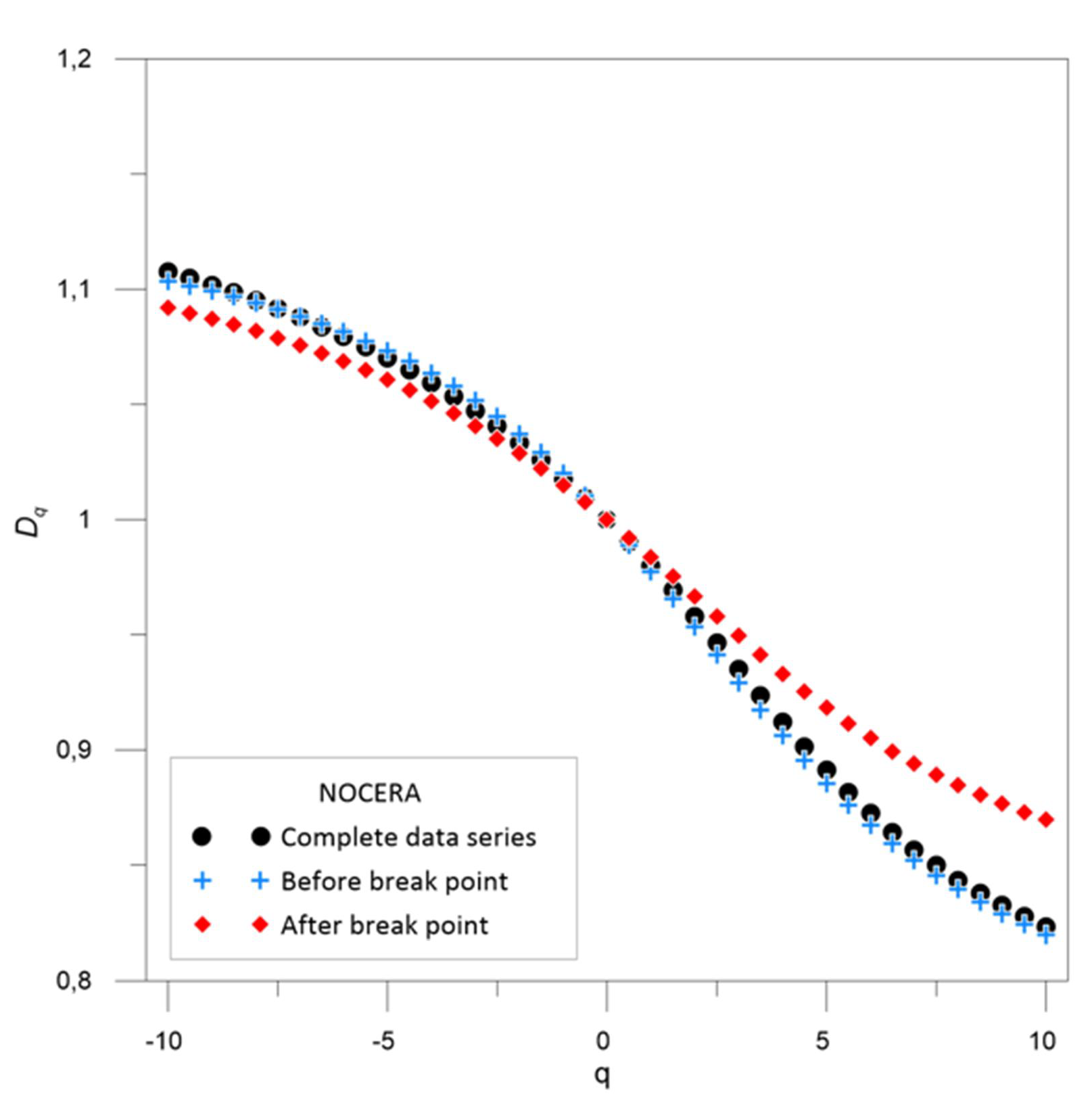
For the Nocera Umbra station, the GFD function Dq for the complete data series is almost coincident with the one obtained for the rainfall data series before the break point. Different values were obtained for the rainfall data series after the break point. The similarity in the behavior of the complete data series and the one before the potential break point means that no real break point exists since the addition of the data after it does not change the general pattern.
The Rénji spectra obtained for the Petrelle station data series are different. In this case, the three data series should be considered as different and thus the break point is real.
No similarities arise between the data series before or after the break points with respect to the complete data series at Spoleto station if all the Dq values are considered. Nevertheless, for negative q values, similar Dq functions are obtained for the data sets before and after the break points in 1969 and 1980. These similitudes are maintained for positive q values for Dq functions of data sets before both break points. Nevertheless, Dq functions are different for positive q values for data sets after the break points, with the one after the inhomogeneity at 1980 being the closest to the Dq function for the complete data series. This behavior means that the break point took place in 1969.
For the Terni station, similar trends of Dq function are found for the complete data series and those before and after the break point year of 1957, respectively. For the former series, similar values are found for q positive values whereas for the latter the similarities arise for negative q values. Different Dq functions are obtained for those series derived from the break point in1962. This behavior implies that the inhomogeneity is placed at 1962 in the Terni extreme rainfall data series.
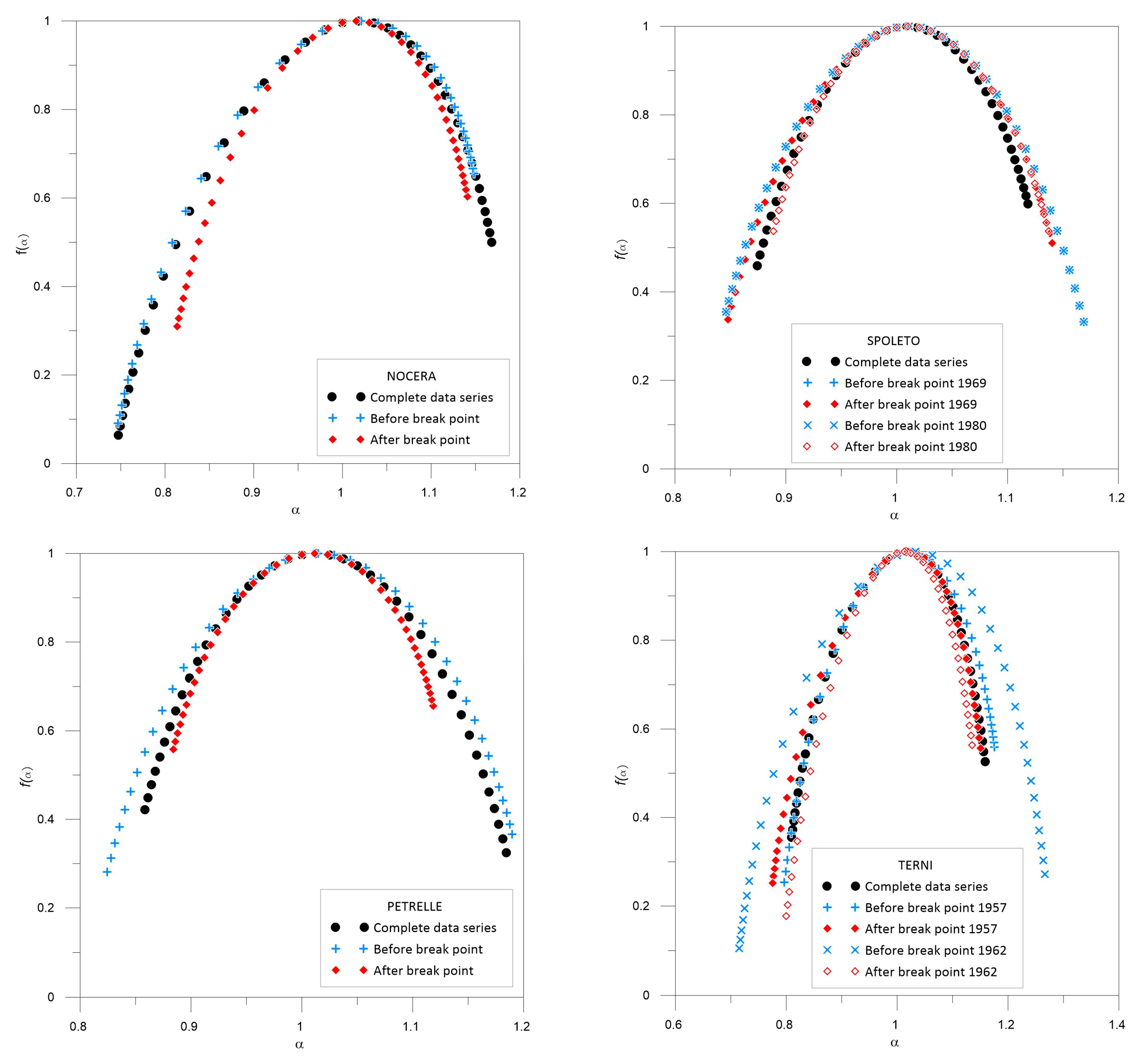
Regarding the shape of the multifractal spectra, similar f(α) are obtained for the Nocera Umbra complete data set and for the one before the break point year. Even though left-side skewed multifractal spectra are found for all the data series, the one for the data set after the break point differs from those previously mentioned.
Different multifractal spectra are also obtained for the Petrelle data sets, where not even the symmetry is similar; the complete data set spectrum is slightly right-skewed, whereas those obtained before and after the break point are skewed in the opposite direction.
Multifractal spectra before the break points appear similar at Spoleto, where the one for the complete data set also differs from those obtained before and after the break points, showing some similarities only for the left side of f(α) after the inhomogeneity in 1980.
Similarities in the multifractal spectra arise for the Terni station for both the complete data set and those before and after the break point in 1957, whereas different results are found for f(α) before and after the break point in 1962 and the whole rainfall data set.
For Nocera Umbra station, the complete extreme rainfall data series shows a negative value for the asymmetry parameter, which means that extreme events are important in the data series, and also there is a high complexity according to the value of parameter w. Even though the asymmetry parameter values are also negative for data sets before and after the break point, the last data series seems to be less influenced by extreme events than the previous one (or even than the complete series). The richness of the process is also lower for the data set after the break point than for both complete and before break point data sets. Almost similar values for all the parameters (αmin, αmax, as and w) were obtained when analyzing both the complete data set and the one before the break point.
For the Petrelle station, different values are obtained for all the parameters and data sets. The influence of extreme events is present in both data sets before and after the break point according to the negative value of the asymmetry parameter (as), whereas the complete data series shows a greater influence of less extreme events, with a positive value of as. The width of the spectra (w) is also different with a loss of richness (lower multifractality) in the complete data set compared to the one before the break point, maybe due to the influence of the data after the break point, where the richness has the lowest value.
For the Terni station, all the spectra exhibit negative values for the asymmetry parameter (as), which implies the dominance of extreme events in all the data series. The values closer to the αmin and αmax parameters are found for the complete data series and for the series before and after 1957, and thus a similar influence by extreme and smooth events can be expected for all the series. Similar complex processes are found according to the values of w. This behavior is not present for data series before and after the break point of 1962, where a loss of multifractality is found after the break point compared to the data series before it. This last data series also shows the strong influence of extreme events according to both the values of as and αmin.
The multifractal spectrum for the Spoleto complete data series shows a negative value for the asymmetry parameter, which is influenced by the presence of extreme events in the data set. The shape changes to a positive value of the asymmetry parameter for the data sets before the break points. The most similar values of all the parameters are found for the complete data set and the one after the break point of 1980.
Authors such us [25] used the variability in the values of α0 and w from the multifractal spectrum to assess changes in climate data series. For all the data sets studied in this work, the values of α0 are always equal to 1 and thus no possible changes can be explained based on these values. Nevertheless, there are differences in the values obtained for the parameter that describes the degree of multifractality of the data series, w. Thus, the differences in the values of this multifractal parameter will be of great importance in deciding if a break point can really be identified in a data series.
According to all the results described above, it can be stated that no inhomogeneity exists in the Nocera extreme annual rainfall data series, whereas the break point detected in the Petrelle data set by the statistical test can be confirmed. For the Spoleto station the behavior is not as clear as in the previous stations if all the parameters are considered, but the closest similarity between complete and split data series is found in 1980, specially for the width of the multifractal spectrum (w) and the fractal dimensions D1 and D2. Thus, the most important inhomogeneity is the one detected by the statistical tests in 1969. For the Terni station, the greatest differences in multifractal properties are found between the complete data series and those obtained considering the inhomogeneity in 1962, especially for the value of w, D1 and D2. Therefore, no break point should be considered in 1957.

5. Conclusions

The multifractal character of rainfall data has been widely studied for extreme annual data of different durations and it is useful when dealing with rainfall predictive modeling or IDF estimation. Thus, the possibility of confirming the existence of a break point previously detected by statistical methods, based on the multifractal behavior of rainfall can help to enhance the results of methods and models that use rainfall as a direct or indirect input, especially, those that depend on the length of the rainfall data series.
The results of this work show that the multifractal characterization of extreme rainfall annual data series can be a suitable tool to decide whether or not an inhomogeneity exists in the data set, especially when there is no agreement in the results from statistical tests. Parametric and non-parametric statistical tests commonly applied to detect shifts in time data series were used to check if any break points were present in extreme annual 24-h rainfall data series in the Umbria region (Italy). For some of the stations considered, no inhomogeneities were found with the statistical tests.
For those stations where only one of the tests detected a break point, or where different years for the break points were identified by the different tests, the maintenance of multifractal parameters’ values was used as the criterion to reject the potential break point. Because multifractal analysis results are sensitive to climate shifts if the spectra parameters of time series divided into subsets differ, the values of the heterogeneity fractal dimension D1, the correlation fractal dimension D2, and the complexity of the data set given by w provide the bases for the decision criteria. If the complete data series maintained the values of D1, D2 or w with respect to any of the split series before or after the break point, it was considered that no inhomogeneity existed. The multifractal behavior of the split series was also found in the complete series. On the contrary, if the values of the multifractal parameters were different among the data series, the break point under consideration was accepted.
According to the results obtained in this work, the multifractal behavior of extreme rainfall data can be considered as an indicator of the changes in the dynamics of the atmospheric processes before and after observed shifts. This is of great importance in models based on extreme rainfall frequency analysis where the existence of a break point in a data series changes the length of it and can influence the estimated values. To make it easier for practitioners and engineers, a software that combine homogeneity tests and multifractal algorithms is being developed.

Author Contributions

Conceptualization, formal analysis, writing original-draft, funding acquisition, supervision—A.P.G.-M.; Funding acquisition, validation—J.E.; resources, data curation, supervision—R.M.; Resources, data curation—C.S.; Methodology, software—J.L.A.-M.; Writing, reviewing and editing—A.F. All authors have read and agreed to the published version of the manuscript.

Funding

This research was funded by the Spanish Ministry of Science, Innovation and Universities, grant number AGL2017-87658-R. And the APC was funded by the same funder.

Acknowledgments

A.P.G.-M. acknowledges the collaboration and hosting of the University of Perugia and specifically, of the Hydrology team of the Department of Civil and Environmental Engineering.

Conflicts of Interest

The authors declare no conflict of interest. The funders had no role in the design of the study; in the collection, analyses, or interpretation of data; in the writing of the manuscript, or in the decision to publish the results.

References

  1. Haktanir, T.; Citakoglu, H. Trend, Independence, Stationarity, and Homogeneity Tests on Maximum Rainfall Series of Standard Durations Recorded in Turkey. J. Hydrol. Eng. 2014, 19, P05014009. [Google Scholar] [CrossRef]
  2. Wijngaard, J.B.; Klein Tank, A.M.G.; Können, G.P. Homogeneity of 20th century European daily temperature and precipitation series. Int. J. Climatol. 2003, 23, 679–692. [Google Scholar] [CrossRef]
  3. Hoerling, M.; Kumar, A.; Eischeid, J.; Jha, B. What is causing the variability in global mean land temperature? Geophys. Res. Lett. 2008, 35, L23712. [Google Scholar] [CrossRef] [Green Version]
  4. Martínez, M.D.; Serra, C.; Burgueño, A.; Lana, X. Time trends of daily maximum and minimum temperatures in Catalonia (NE Spain) for the period 1975–2004. Int. J. Climatol. 2010, 30, 267–290. [Google Scholar]
  5. Geng, Q.; Wu, P.; Zhao, X. Spatial and temporal trends in climatic variables in arid areas of northwest China. Int. J. Climatol. 2016, 36, 4118–4129. [Google Scholar] [CrossRef]
  6. Swanson, K.L.; Tsonis, A.A. Has the climate recently shifted? Geophys. Res. Lett. 2009, 36, L06711. [Google Scholar] [CrossRef] [Green Version]
  7. Morozova, A.L.; Valente, M.A. Homogenization of Portuguese long-term temperature data series: Lisbon, Coimbra and Porto. Earth Syst. Sci. Data 2012, 4, 187–213. [Google Scholar] [CrossRef] [Green Version]
  8. Guo, Y. Updating Rainfall IDF Relationships to Maintain Urban Drainage Design Standards. J. Hydrol. Eng. 2006, 11, 506–509. [Google Scholar] [CrossRef]
  9. Hassan, H.W.; Nile, B.K.; Al-Masody, B.A. Study the climate change effect on storm drainage networks by storm water management model [SWMM]. Environ. Eng. Res. 2017, 22, 393–400. [Google Scholar] [CrossRef]
  10. Adamowski, K.; Bougadis, J. Detection of trends in annual extreme rainfall. Hydrol. Process. 2003, 17, 3547–3560. [Google Scholar] [CrossRef]
  11. Fujibe, F.; Yamazaki, N.; Katsuyama, M.; Kobayashi, K. The increasing trend of intense precipitation in Japan based on four-hourly data for a hundred years. Sci. Online Lett. Atmos. SOLA 2005, 1, 41–44. [Google Scholar] [CrossRef] [Green Version]
  12. Wang, B.; Ding, Q.; Jhun, J.G. Trends in Seoul (1778–2004) summer precipitation. Geophys. Res. Lett. 2006, 33, L15803. [Google Scholar] [CrossRef] [Green Version]
  13. Burn, D.H.; Mansour, R.; Zhang, K.; Whitfield, P.H. Trends and variability in extreme rainfall events in British Columbia. Can. Water Resour. J. 2011, 36, 67–82. [Google Scholar] [CrossRef]
  14. Douglas, E.M.; Fairbank, C.A. Is precipitation in northern New England becoming more extreme? Statistical analysis of extreme rainfall in Massachusetts, New Hampshire, and Maine and updated es- timates of the 100-year storm. J. Hydrol. Eng. 2011, 16, 203–217. [Google Scholar] [CrossRef] [Green Version]
  15. Nandargi, S.; Dhar, O.N. Extreme rainfall events over the Himalayas between 1871 and 2007. Hydrol. Sci. J. 2011, 56, 930–945. [Google Scholar] [CrossRef] [Green Version]
  16. Yavuz, H.; Erdogan, S. Spatial analysis of monthly and annual precipitation trends in Turkey. Water Resour. Manag. 2012, 26, 609–621. [Google Scholar] [CrossRef]
  17. Xu, Z.X.; Takeuchi, K.; Ishidaira, H. Monotonic trend and step changes in Japanese precipitation. J. Hydrol. 2003, 279, 144–150. [Google Scholar] [CrossRef]
  18. Shadmani, M.; Marofiand, S.; Roknian, M. Trend analysis in reference evapotranspiration using Mann–Kendall and Spear- man’s Rho tests in Arid Regions of Iran. Water Resour. Manag. 2012, 26, 211–224. [Google Scholar] [CrossRef] [Green Version]
  19. Piccarreta, M.; Lazzari, M.; Pasini, A. Trends in daily temperature extremes over the Basilicata region (southern Italy) from 1951 to 2010 in a Mediterranean climatic context. Int. J. Climatol. 2015, 35, 1964–1975. [Google Scholar] [CrossRef]
  20. Koutsoyiannis, D. Climatic change, the hurst phenomenon, and hydrological statistics. Hydrol. Sci. J. 2003, 48, 3–24. [Google Scholar] [CrossRef]
  21. Koutsoyiannis, D. Nonstationarity versus scaling in hydrology. J. Hydrol. 2006, 324, 239–254. [Google Scholar] [CrossRef] [Green Version]
  22. Haddad, O.B.; Moravej, M. Discussion of “Trend, Independence, Stationarity, and Homogeneity Tests on Maximum Rainfall Series of Standard Durations Recorded in Turkey” by Tefaruk Haktanir and Hatice Citakoglu. J. Hydrol. Eng. 2015, 20, 07015016. [Google Scholar] [CrossRef]
  23. Hamed, K.H. Trend detection in hydrologic data: The Mann–Kendall trend test under the scaling hypothesis. J. Hydrol. 2008, 349, 350–363. [Google Scholar] [CrossRef]
  24. Baranowski, P.; Krzyszczak, J.; Slawinski., C.; Hoffmann, H.; Kozyra, J.; Nierόbca, A.; Siwek, K.; Gluza, A. Multifractal analysis of me- teorological time series to assess climate impacts. Clim. Res. 2015, 65, 39–52. [Google Scholar] [CrossRef] [Green Version]
  25. Krzyszczak, J.; Baranowski, P.; Zubik, M.; Kazandjiev, V.; Georgieva, V.; Sławiński, C.; Siwek, K.; Kozyra, J.; Nierόbca, A. Multifractal characterization and comparison of meteorological time series from two climatic zones. Theor. Appl. Climatol. 2018, 137, 1811–1824. [Google Scholar] [CrossRef] [Green Version]
  26. García-Marín, A.P.; Jiménez-Hornero, F.J.; Ayuso, J.L. Applying multifractality and the self-organized criticality theory to describe the temporal rainfall regimes in Andalusia (southern Spain). Hydrol. Process. 2008, 22, 295–308. [Google Scholar] [CrossRef]
  27. García-Marín, A.P.; Estévez, J.; Jiménez-Hornero, F.J.; Ayuso-Muñoz, J.L. Multifractal analysis of validated wind speed time series. Chaos 2013, 23, 13133–21505. [Google Scholar] [CrossRef]
  28. Jiménez-Hornero, F.J.; Jiménez-Hornero, J.E.; de Ravé, E.G.; Pavon-Dominguez, P. Exploring the relationship between nitrogen dioxide and ground-level ozone by applying the joint multifractal analysis. Environ. Monit. Assess. 2010, 167, 675–684. [Google Scholar] [CrossRef]
  29. Morbidelli, R.; Saltalippi, C.; Flammini, A.; Corradini, C.; Wilkinson, S.M.; Fowler, H.J. Influence of temporal data aggregation on trend estimation for intense rainfall. Adv. Water Resour. 2018, 122, 304–316. [Google Scholar] [CrossRef]
  30. Buishand, T.A. Some methods for testing the homogeneity of rainfall records. J. Hydrol. 1982, 58, 11–27. [Google Scholar] [CrossRef]
  31. Alexandersson, H. A homogeneity test applied to precipitation data. Int. J. Climatol. 1986, 6, 661–675. [Google Scholar] [CrossRef]
  32. Khaliq, M.N.; Ouarda, T.B.M.J. On the critical values of the standard normal homogeneity test (SNHT). Int. J. Climatol. 2007, 27, 681–687. [Google Scholar] [CrossRef]
  33. Pettitt, A.N. A non-parametric approach to the change-point problem. Appl. Stat. 1979, 28, 126–135. [Google Scholar] [CrossRef]
  34. Brunetti, M.; Maugeri, M.; Nanni, T. Variations of temperature and precipitation in Italy from 1866 to 1995. Theor. Appl. Climatol. 2000, 65, 165–174. [Google Scholar] [CrossRef]
  35. Partal, T.; Kahya, E. Trend Analysis in Turish Precipitation Data. Hydrol. Process. 2006, 20, 2011–2026. [Google Scholar] [CrossRef]
  36. Karpouzos, D.K.; Kavalieratou, S.; Babajimopoulos, C. Trend Analysis of Precipitation Data in Pieria Region (Greece). Eur. Water 2010, 30, 31–40. [Google Scholar]
  37. McGilchrist, C.C.; Woodyer, K.D. Note on a Distribution-Free CUSUM Technique. Technometrics 1975, 17, 321–325. [Google Scholar] [CrossRef]
  38. Wang, X.; Yang, X.; Liu, T.; Li, F.; Gao, R.; Duan, L.; Luo, Y. Trend and extreme occurrence of precipitation in a midlatitude Eurasian steppe watershed at various time scales. Hydrol. Process. 2014, 28, 5547–5560. [Google Scholar] [CrossRef]
  39. Casas-Castillo, M.C.; Rodríguez-Solá, R.; Navarro, X.; Russo, B.; Lastra, A.; González, P.; Redaño, A. On the consideration of scaling properties of extreme rainfall in Madrid (Spain) for developing a generalized intensity-duration-frequency equation and assessing probable maximum precipitation estimates. Theor. Appl. Climatol. 2018, 131, 573–580. [Google Scholar] [CrossRef]
  40. García-Marín, A.P.; Morbidelli, R.; Saltalippi, C.; Cifrodelli, M.; Estévez, J.; Flammini, A. On the choice of the optimal frequency analysis of annual extreme rainfall by multifractal approach. J. Hydrol. 2019, 575, 1267–1279. [Google Scholar] [CrossRef]
  41. Carmona-Cabezas, R.; Ariza-Villaverde, A.B.; Gutiérrez de Ravé, E.; Jiménez-Hornero, F.J. Visibility graphs of ground-level ozone time series: A multifractal analysis. Sci. Total Environ. 2019, 661, 138–147. [Google Scholar] [CrossRef] [PubMed]
  42. Feder, J. Fractals; Plenum: New York, NY, USA, 1988. [Google Scholar]
  43. Davis, A.; Marshak, A.; Wiscombe, W.; Cahalan, R. Multifractal characterization of non stationarity and intermittency in geophysical fields: Observed, retrieved or simulated. J. Geophys. Resour. 1994, 99, 8055–8072. [Google Scholar] [CrossRef]
  44. Herrera-Grimaldi, P.; García-Marín, A.P.; Estévez, J. Multifractal analysis of diurnal temperature range over Southern Spain using validated datasets. Chaos 2019, 29, 063105. [Google Scholar] [CrossRef] [PubMed]
  45. Ding, M.; Grebogi, C.; Ott, E.; Sauer, T.; Yorke, J.A. Estimating correlation dimension from a chaotic time series: When does plateau onset occur? Physica D 1993, 69, 404–424. [Google Scholar] [CrossRef]
Figure 1. Rain gauges in the Umbria region used in this work.
Water 12 01030 g001
Figure 2. Results obtained from the sequential Mann–Kendall test in the Spoleto and Terni stations.
Water 12 01030 g002
Figure 3. Step changes detected by the Mann–Whitney U test at the Nocera Umbra, Spoleto, Petrelle and Terni stations.
Water 12 01030 g003
Figure 4. Results obtained at the Bastia Umbra and Terni stations after applying the CUSUM test.
Water 12 01030 g004
Figure 5. Multifractal dimensions functions Dq for the complete data series and also for the rainfall series before and after the break points detected in the Nocera Umbra, Petrelle, Spoleto and Terni stations.
Water 12 01030 g005
Figure 6. Multifractal spectra f(α) for the complete rainfall data series and also for the rainfall data series before and after the break points detected in the Nocera Umbra, Petrelle, Spoleto and Terni stations.
Water 12 01030 g006
Table 1. Stations selected for the work and the period of data considered.
Station.Period (Years) Considered
Bastia Umbrafrom 1966 to 2017
Bevagnafrom 1967 to 2017
Nocera Umbrafrom 1961 to 2017
Petrellefrom 1951 to 2017
Ponte Nuovo di Torgianofrom 1954 to 2017
Spoletofrom 1949 to 2017
Ternifrom 1952 to 2017
Todifrom 1948 to 2017
Table 2. Results obtained for the parametric Buishand range (BR) and Standard Normal Homogeneity (SNH) tests; the statistics Q and T0 and their critical values Qc and T0c are also shown.
StationBRTSNHT
QQcT0T0c
Bastia Umbra0.8621.2716.6898.480
Bevagna0.7461.2702.6268.456
Nocera0.6501.2733.0948.586
Petrelle0.9781.2773.9708.768
Ponte0.6151.2762.1828.717
Spoleto1.2951.2777.5468.784
Terni1.0881.2767.5058.735
Todi0.7391.2783.7948.814
Table 3. Results obtained after applying the Pettitt test.
StationPettitt Test
KK0.05
Bastia Umbra213.0267.5
Bevagna170.0259.9
Nocera194.0306.7
Petrelle322.0390.4
Ponte152.0356.1
Spoleto435.0399.1
Terni276.0373.1
Todi237.0461.8
Table 4. Summary of the years in which break points were detected by the applied tests.
StationParametric TestsNon-Parametric Tests
BRSNHPTSQMKMWUCUSUM
Bastia Umbra------
Bevagna------
Nocera Umbra----1968-
Petrelle----1994-
Ponte------
Spoleto1977-196919801969-
Terni---19571962-
Todi------
Table 5. Main results obtained for the Rénji spectrum of the extreme rainfall data series for which break points were detected by the statistical tests.
StationComplete Data SeriesBefore Break Point SeriesAfter Break Point Series
D1D2D0-D1D0-D2D1D2D0-D1D0-D2D1D2D0-D1D0-D2
Nocera Umbra19680.9800.9580.0200.0420.9770.9530.0230.0470.9840.9670.0160.033
Petrelle19940.9880.9750.0120.0250.9850.9710.0150.0290.9880.9770.0120.023
Terni19570.9800.9600.0200.0400.9800.9590.0200.0410.9790.9550.0210.045
19620.9650.9300.0350.0700.9860.9720.0140.028
Spoleto19690.9910.9810.0090.0190.9890.9770.0110.0230.9890.9780.0110.022
19800.9890.9770.0110.0230.9900.9810.0100.019
Table 6. Main results obtained for the multifractal spectrum of the extreme rainfall data series for which break points were detected by the statistical tests.
StationComplete Data SeriesBefore Break Point SeriesAfter Break Point Series
αminαmaxaswαminαmaxaswαminαmaxasw
Nocera Umbra19680.747311.16829−0.435610.420980.746971.14838−0.564160.401420.813721.14083−0.294070.32712
Petrelle19940.858471.184290.096500.325810.824461.18982−0.085290.365360.884171.11864−0.098680.23448
Terni19570.809521.15864−0.170810.349130.796421.17564−0.305610.379220.775231.15035−0.304850.37513
19620.714931.26671−0.166860.551780.799811.13520−0.386380.33539
Spoleto19690.874271.11828−0.139990.244010.846081.168690.022760.322610.847761.14035−0.172510.29258
19800.846081.168690.022760.322610.888811.13704−0.000220.24823

