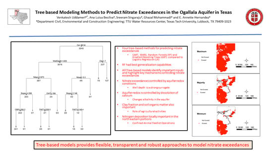
Tree-Based Modeling Methods to Predict Nitrate Exceedances in the Ogallala Aquifer in Texas
by
 , and
, and
Venkatesh Uddameri
* ,
,
Ana Luiza Bessa Silva
,
Sreeram Singaraju
,
Ghazal Mohammadi
 and
and
E. Annette Hernandez
Department of Civil, Environmental and Construction Engineering, Tech University, Lubbock, TX 79409-1023, USA
*
Author to whom correspondence should be addressed.
Water 2020, 12(4), 1023; https://doi.org/10.3390/w12041023
Submission received: 6 March 2020
/
Revised: 29 March 2020
/
Accepted: 31 March 2020
/
Published: 3 April 2020
(This article belongs to the Section Hydrology)
Abstract
:The performance of four tree-based classification techniques—classification and regression trees (CART), multi-adaptive regression splines (MARS), random forests (RF) and gradient boosting trees (GBT) were compared against the commonly used logistic regression (LR) analysis to assess aquifer vulnerability in the Ogallala Aquifer of Texas. The results indicate that the tree-based models performed better than the logistic regression model, as they were able to locally refine nitrate exceedance probabilities. RF exhibited the best generalizable capabilities. The CART model did better in predicting non-exceedances. Nitrate exceedances were sensitive to well depths—an indicator of aquifer redox conditions, which, in turn, was controlled by alkalinity increases brought forth by the dissolution of calcium carbonate. The clay content of soils and soil organic matter, which serve as indicators of agriculture activities, were also noted to have significant influences on nitrate exceedances. Likely nitrogen releases from confined animal feedlot operations in the northeast portions of the study area also appeared to be locally important. Integrated soil, hydrogeological and geochemical datasets, in conjunction with tree-based methods, help elucidate processes controlling nitrate exceedances. Overall, tree-based models offer flexible, transparent approaches for mapping nitrate exceedances, identifying underlying mechanisms and prioritizing monitoring activities.
1. Introduction
Nitrate (NO3-N) is a widespread environmental contaminant that is commonly detected in groundwater supplies and can cause severe health effects, both in children and adults [1]. Nitrates in groundwater can arise from multiple sources, including, but not limited to, the use of fertilizers, improper waste management practices from animal feed operations, inadequate treatment of household wastewater prior to its discharge in the environment, as well as from natural sources (decay or natural organic matter). Many groundwater dependent public water supply systems in the US and particularly in the rural parts of Texas have seen increases in the violation of nitrate drinking water quality standards over the last few decades [2]. In addition, over 13 million households in the United States (approximately 15% of the nation’s population) rely on unregulated private water wells to meet their drinking water needs [3]. A large majority of this population is rural and susceptible to exposure to elevated nitrate concentrations through their drinking water sources [4]. Reliance on private water wells is even higher in under-developed and developing nations and, as such, efforts to characterize nitrate in groundwater aquifers are actively being pursued by several local, state and national agencies worldwide [5,6]. Intensification of agricultural activities for both food and energy will further increase the risks of nitrate contamination in aquifers across the world [7,8,9].
Nitrate is mobile and fairly recalcitrant, especially in shallow groundwater systems that typically tend to be under oxidizing conditions. Nitrate exhibits the ability to spread over large areas and cannot be treated in-situ using conventional plume scale treatment technologies [10]. Therefore, individual homeowners are often required to install costly point-of-use treatment systems to mitigate nitrate risks arising from the ingestion of contaminated groundwater [11,12]. However, as nitrate is colorless and odorless, many people do not realize the risk of nitrate contamination and are unwittingly exposed to elevated levels of nitrate over long periods of time [13]. Therefore, nitrate contamination must be prevented through proper land management practices. Additionally, areas with a high susceptibility to nitrate pollution must be carefully delineated, with the goal of increasing public awareness regarding elevated health risks arising from nitrate exposures. Such an effort is also useful to prioritize monitoring activities and ensure that the limited fiscal and logistic resources are being used in a prudent manner.
Mapping the susceptibility of aquifers to nitrate contamination is an essential step in mitigating and managing nitrate contamination. Multi-criteria decision making (MCDM) methods, such as DRASTIC [14], have been widely used to map aquifer vulnerability [15]. Intrinsic vulnerability methods do not account for chemical specific characteristics; therefore, approaches that account for existing pollution have also been proposed in the literature. In particular, logistic regression models have been extensively used, albeit with a mixed degree of success, to calculate the probability of the exceedance of a pre-defined nitrogen (or some other contaminant) threshold [12,16,17,18,19,20,21,22,23,24,25,26,27].
The main reasons for the popularity of logistic regression techniques for aquifer vulnerability assessment include its ability to deal with censored data and the availability of computer programs to perform the necessary calculations. Furthermore, the resulting equation can be easily embedded into a geographic information system (GIS) to develop aquifer vulnerability maps. While logistic regression is easy to implement, the explanatory (independent) variables used to predict the probability of nitrate exceedance must be carefully selected a priori. In addition, the logit function is assumed to be a linear function of the explanatory variables and a single global equation is used model the entire dataset. As such, it may have limited capabilities for modeling the nonlinear dependencies that arise locally, due to aquifer heterogeneity and geochemical variability at the field scale.
Tree-based classification methods work on the principle of recursively partitioning the dataset, such that data is clustered as closely as possible with other similar data, while being as far apart as possible from dissimilar data that are clustered separately. A primary advantage of the tree-based models lies in the fact that the structure of the model need not be specified a priori [28]. Tree-based modeling can be used to extract the underlying structure of the model and identify important variables influencing the output. The tree structure also makes it easy to understand the nonlinear relationships between input parameters and the output, as well as the interactions between various input parameters [29]. In addition, tree-based models require very little data preparation and can handle outliers and missing values. Unlike many other machine learning methods, normalization of data is not needed for tree-based models. Tree-based models can be constructed with limited data, but are also capable of mining extremely large datasets. Tree-based algorithms do not use a single (global) equation, but fit multiple local models for different data partitions. This allows them to model nonlinearities in the dataset, arising from aquifer heterogeneity and geochemical variability. As such, they can be useful to not only predict nitrate contamination susceptibility, but also help elucidate underlying processes and controls, which are useful for the subsequent design of treatment systems, as well as to develop and refine groundwater quality monitoring programs.
The advantage of tree-based methods in water quality studies has been recognized. The classification and regression tree (CART) approach [30] has been applied to water quality problems [31]. In particular, Burow et al. [32] used the CART algorithm as an exploratory tool to identify factors affecting nitrate concentrations in principal aquifers in the US. The multi-adaptive regression splines (MARS) combines recursive partitioning and spline-based fitting to develop highly nonlinear and accurate relationships between input and output parameters [33]. Furthermore, the MARS model, with its tree-structure, provides valuable insights into the relationships between input and output variables and identify important input subsets. Given these advantages, there is a growing interest in using the tree-based MARS in water quality and groundwater studies [34,35,36]. The utility of tree-based classifiers can be further enhanced using bagging and boosting techniques, used by ensemble-based classifiers such as the random forests (RF) [37] and the gradient boosting trees (GBT) algorithms [38,39]. The RF algorithm has been successfully used for modeling nitrate contamination in groundwater waters [26,40,41]. The boosted trees method has also been used to predict the susceptibility of nitrate pollution [42,43].
While recent studies indicate that tree-based models hold promise for assessing water quality and delineating aquifer vulnerability, there is still a need to evaluate the feasibility of these modeling schemes at other locations and geographies, to gain confidence in their use. As nitrogen concentrations are affected by a variety of physical, chemical and biological processes, evaluating the ability of various tree-based models to elucidate underlying processes and mechanisms from integrated soil, hydrogeological and geochemical datasets has not been explored to date, and is an important research gap that this study seeks to address. Therefore, this study employs four tree-based modeling techniques—classification and regression trees (CART), multi-adaptive regression splines (MARS), gradient boosting trees (GBT) and random forests (RF) to model nitrate exceedances in the Ogallala Aquifer in the Southern High Plains (SHP) region of Texas (see Figure 1), and benchmarks the results against the commonly used logistic regression (LR) technique using a comprehensive multivariate soil, hydrogeological and geochemical dataset.
The Southern High Plains (SHP) region of Texas is an area of intense agricultural activity and a top producer of cotton, corn and beef products in the nation [44]. The SHP region has intense agricultural activity and well drained soils, and is very conducive to nitrate pollution from anthropogenic activities [45,46]. In addition, the mineralization and nitrification of old (pre-cultivation era) soil organic nitrogen, due to enhanced microbial activity brought forth by increased soil wetness from irrigated agriculture, is also known to affect nitrogen recycling in SHP and increase nitrate contamination of aquifers [47]. Elevated levels of nitrate (in excess of maximum contaminant level of 10 mg/L as NO3-N) are a widespread problem in the SHP aquifer [24]. Therefore, this region forms an ideal testbed, to evaluate different approaches to predict aquifer vulnerability to nitrate exceedances.
2. Methods
2.1. Logistic Regression (LR)
Logistic regression is a popular technique for mapping aquifer vulnerability; therefore, it is used here to benchmark the performance of tree-based modeling schemes. For a dichotomous random variable, Y, that takes two values (0, 1), the odds (O) of favoring a value of 1 (exceedance) and the logit (L) can be written as:
Logistic regression refers to models in which the logit is the state variable (output) and is linearly related to a set of m predictors (X1, X2,…, Xm) as:
An estimate of the probability, P(Y = 1), can be obtained by reversing the logit transformation
Note that the logistic regression approach assumes the logit is a linear function of a set of independent variables, which must be specified a priori. The model parameters (intercept and model coefficients), estimated using the maximum likelihood approach and statistical methods for evaluating the significance of model coefficients, are well established for this technique [48] and are not repeated here, in the interest of brevity.
2.2. Feature Selection for Logistic Regression Model Specification
The selection of appropriate features is an import aspect of LR modeling. While step-wise approaches have been popular, there is a growing recognition that these methods can discard important variables, select variables that exhibit a high degree of multicollinearity and lead to model overfitting—i.e., the model performs well on training data, but has poor generalization abilities [49]. Physical considerations, in conjunction with the correlation matrix and a filter based variable importance measure [50], were used to select a subset of input variables to be included in the LR model. This independent feature selection also provides a comparison to automatic feature selection and variable importance measures that are in-built into tree-based methods.
2.3. Single-Tree-Based Methods
2.3.1. Classification and Regression Trees (CART)
The classification and regression trees (CART) method is a recursive partitioning technique, wherein output data assigned to a particular node are partitioned into two groups, using a cut-off value of an independent variable. The forward partitioning is carried out, so that data points within a group are clustered as closely as possible to each other and as far as possible from the data points in the other group [51]. The CART model cycles through each independent variable and evaluates various cut-offs to identify the most appropriate variable for a given node. The cut-off at which the split is made is chosen such that the difference in deviance between the two splits is maximized. The tree is grown by successively applying the method at each node that is created in the previous stage, until the tree cannot grow anymore.
The CART model is referred to as a greedy algorithm, because it optimizes the error locally at each node, rather than optimizing the error structure associated with the overall tree. Each node within a tree has a partitioning rule which is defined through minimization of the relative error (RE), which is given as follows:
where yL and yR are left and right partitions with L and R observations and yLm and yRm are the mean values for left and right partitions. The decision rule is a point in some input variable that is used to determine left and right branches [52]. While the model cycles through all initially supplied input variables, it may only pick a subset of the inputs (i.e., those that provide the optimal separation at each node of the tree). Therefore, the approach also performs the task of data reduction and helps identify important variables. Input variables that are used to make primary (higher-level) partitions are more important, as they are used to partition a larger subset of data. Additionally, a variable used for multiple partitions influences the output in a more nonlinear fashion than one that is used for a single or fewer partitions.
The complexity of the tree is defined by the number of nodes and the number of input parameters used to make the split and is quantified using the complexity parameter, which measures the tradeoff between the model structure and predictive capabilities of the tree. The initial tree developed by the CART model is typically too complex to be of practical use. While this tree may be able to correctly learn the patterns in the training data, it usually lacks generalization capabilities. Therefore, in the backward pass, the tree is pruned, to reduce its complexity. In the pruning step, the branches are removed, and data are aggregated at higher levels. A k-fold cross-validation approach is used to evaluate the predictive errors associated with a particular level of pruning, as compared to a tree with no splits (i.e., maximal error), and is used to identify a suitable pruned version as the final model [53]. A CART model typically provides a single valued estimate of a continuous output, or probability values for a discrete output that can be categorized as 0 and 1.
2.3.2. Multi-Adaptive Regression Splines (MARS)
The multi-adaptive regression splines, or MARS, is another recursive partitioning technique that integrates tree-based classification concepts with regression and splines-based curve-fitting approaches. It is an adaptive nonlinear regression procedure for fitting relationships between a response variable and a set of predictors using piecewise basis functions [33]. The process is similar to the CART approach, in that a cut-off value (hinge) of an independent variable is used to induce a kink in the relationship, in order to capture the underlying nonlinearity in the input-output relationship. The cut-offs are used to develop basis functions (BFs), an example of which is given in Equation (6).
The BFs can also be viewed as a new predictor matrix in which the columns of the BFs replace each predictor variable in the original data [54]. More than one knot can be specified to fit complex nonlinear relationships. Multiplicative hinges involving two or more model inputs can be used to model nonlinearities arising from interactive effects. In a manner similar to CART, the independent variables to be included in the BFs and their corresponding cut-off values are estimated simultaneously by the model. The BFs are identified sequentially and automatically in the forward pass and the model is built using linear regression (for continuous output), or logistic regression when the output is a discrete variable [55]. In the backward step, the model is made parsimonious by removing certain kinks, but using higher-order splines to capture noted nonlinearities in the input-output relationships. As the MARS model uses logistic regression for binary classification in a piece-meal fashion, the output produced by the model corresponds to the probability of exceedance, which can be categorized into a binary output using a suitable cut-off value.
2.4. Ensemble-Based Methods
In single tree-based methods, the focus is on developing one final model (tree), that provides sufficiently accurate predictions and also satisfies the principle of parsimony. Tree-based models may perform extremely well on a subset of data and very poorly on another subset within the same dataset. Ensemble-based methods try to improve model predictions by developing multiple tree-based models and aggregating them to provide predictions. The basic premise of aggregation is that different models, which perform differently on subsets of the data, can be effectively combined to offer a best set of predictions over the entire range of data. Bagging and boosting are two commonly used approaches for building ensemble models [56]. Bootstrap aggregation or bagging is based on the idea of creating an ensemble of trees, by bootstrapping the data and then using a voting scheme to perform classification [57]. The approach primarily focuses on reducing the variance of error rather than the bias in the predictions. While boosting also creates an ensemble of models, it seeks to draw samples intelligently by iteratively giving more weight to incorrect predictions, as it minimizes errors. Bagging is based on deep trees (strong learners) while boosting tends to work with shallow trees (weak learners) and could also include stumps (i.e., a tree with a single node). The random forest (RF) is an advanced bagging algorithm [38] that is now considered as a standard, widely used approach to bagging. There have been several variants of boosting proposed in the literature [58,59], but the gradient-boosting trees (GBT) method [39,60] has gained popularity in machine learning literature, particularly given its flexibility and the ability to solve complex problems [61], and is adopted here as well.
2.5. Random Forests (RF)
The basic idea behind the random forests (RF) algorithm is to build a set of uncorrelated trees using a CART-like procedure. Deep trees with several nodes tend to overfit the data (i.e., memorize the dataset rather than generalize the relationship) and, as such, have low bias but high variance. The RF algorithm applies the bagging concept to CART and draws random samples with replacement of the training dataset to develop a set of trees. In the traditional bootstrapping approach, only the observations (training data) are obtained via replacement and all the predictors are retained during each realization. While this approach can help reduce the variance without significantly increasing the bias, correlation among trees cannot be guaranteed, especially if a set of predictors has a very high influence. Therefore, the RF algorithm uses a “feature bagging” approach, in which not only are the data sampled randomly, but the predictors are also sampled randomly during each realization.
Each tree in the random forest (RF) is built using the partitioning rule given in Equation (5), based on various subsets of data records and attributes. For a binary classification, the output from each tree can be classified as either 0 (non-exceedance) or 1 (exceedance). The final classification of the random forest is based on a majority vote. Mathematically, if K trees within the Random Forest comprising of N total trees predict 0 and K > N/2 (i.e., majority), then the output of the RF is non-exceedance, otherwise it is categorized as exceedance (see Equation (7)). It is therefore always useful to specify the total number of trees as an odd number to avoid ties.
The RF algorithm uses the observations left out of resampling (referred to as the out of bag or OOB samples) to estimate the generalization error. The use of out-of-bag (OOB) samples to estimate the predictive error eliminates the need for cross-validation, and as such, improves the computational efficiency of the algorithm. The RF algorithm does not yield a single tree or a simple formula and from this standpoint, it can be viewed as a black-box algorithm. However, as several subsets of models with different predictors are constructed during the training phase, useful insights can be drawn with regards to the underlying structure in the dataset. In particular, the OOB error is useful to establish the importance of different variables used as predictors.
2.6. Gradient Boosting Trees (GBT)
Boosting is an adaptive method for combining many simple models to improve predictive performance [62]. As the name suggests, gradient boosting trees (GBT), or boosting regression trees, combine the tree-based predictive algorithms with the boosting approach. The GBT algorithm is capable of fitting highly nonlinear relationships and can effectively deal with outliers and missing data. A GBT algorithm can select an appropriate set of variables from a large set of predictors, and can also automatically identify interactions among inputs. Therefore, GBT can be viewed as a complementary ensemble method to the RF algorithm. Boosting algorithms proceed sequentially and in a stage-wise manner, to aggregate the final model.
The GBT method [63] starts by building an initial tree-based model of a given tree size, that seeks to best explain the variance in the data. The tree size is controlled by the user-specified tree complexity parameter (tc). The tree complexity defines the extent of interactions allowed in the model. A loss function (e.g., deviance) is used to identify the best-fit model at each stage. Once the first model is created, the difference between the model predictions and the observations (i.e., residuals or misclassifications) are calculated. In the second stage, another tree model is fit to predict the misclassifications obtained from the first stage. The second tree could potentially use a completely new set of predictors to model the residuals. The residuals remaining after the first two stages are fit to another tree in the third stage and the process is repeated several times. The boosting process is said to be stage-wise, because the trees constructed at earlier stages are left unchanged when the residuals (misclassifications) arising from them are minimized at a later stage. The final GBT model is a linear combination of hundreds or thousands of trees, and can therefore be thought of as a linear regression, where each term is a tree [64]. If the GBT algorithm employs a total of M trees, the function approximation at the mth stage can be mathematically expressed as:
where F(X) is the final output of the GBT model at stage m, Fm−1(X) is the model constructed at stage m − 1 (previous stage) and h(X,am) is the model constructed at stage m, whose parameters are am and h is a decision tree and am corresponds to attributes used for splitting the nodes and their cut-off values. The model starts off with an initial guess Fo(X) for m = 1 and each h(X,am) can be seen as a successive boost based on preceding steps, aimed at improving the overall predictive accuracy. The learning rate multiplier is obtained as part of the parameter estimation process by minimizing a loss function over the training dataset [63].
While the GBT algorithm follows the steepest descent towards the minimum error, the process works best if the movement proceeds slowly along the gradient. This slow movement towards the minimal error ensures that highly curvilinear relationships are accurately modeled in a piece-wise linear manner. Therefore, the contribution of each tree is shrunk using a learning rate (lr) that is assumed to be much less than unity. The prediction of the final value is computed by summing up the contributions of all trees multiplied by the learning rate. The GBT algorithm is rendered stochastic by randomly sub-setting the data to fit each new tree [65]. Stochasticity is seen to reduce the variance and helps improve the predictive capabilities of the final model. The GBT algorithm is optimized by jointly altering the tree complexity (tc), learning rate (lr) and the number of trees (nt). While the final model cannot be readily visualized (black box mode), the output from the GBT approach can be used to identify important variables and their effects on the output, as well as significant interactions amongst the predictors.
2.7. Model Evaluation and Comparison
The evaluation of binary classifiers is commonly carried out by constructing contingency tables and evaluating how the model classifications compare to actual observations [66]. The receiver operating characteristics (ROC) curve can be used to identify an optimal cut-off probability, to discriminate between exceedance and non-exceedance when the dataset is unbalanced. In this study, the cut-off probabilities were selected such that they minimized the distance from the ideal sensitivity and ideal specificity values of unity. The 2 × 2 contingency tables were then created to compare observed and model predicted non-exceedances. The Barnard’s exact test of independence, the odds-ratio and other classifier performance measures, such as sensitivity, specificity, recall rate and precision, were used to evaluate the models [67]. The average performance of the tree-based classifiers and their ability to perform better than random guessing was evaluated using the area under the ROC curve (AUC). AUC values less than 0.5 indicate that the classifier is no better than random guessing, and a score of 1 indicates a perfect discrimination of exceedance and non-exceedance values [54].
2.8. Data Compilation and Predictor Variables Selection
Nitrate concentrations measured at 101 wells, as part of a statewide groundwater monitoring program in Texas, were adopted in this study, to evaluate nitrate contamination in the Ogallala aquifer in Texas. As nitrate and other chemical constituents were only sampled synoptically, measurements made over a period of 1995–2015 were used in this study, to obtain sufficient spatial coverage across the aquifer. A comparison of values at wells with multiple measurements indicated that nitrate values had not changed significantly over the average time period (maximum values were typically less than 1.15 average value). As such, the temporal average nitrate value at each well were taken as representative values for further analysis. A cut-off of 10 mg/L nitrate-nitrogen, corresponding to the maximum contaminant level (MCL), or the drinking water standard, was adopted here to create a binary variable called exceedance. The exceedance variable therefore represents whether the water from the well is in violation of the drinking water standard. The binary exceedance variable was the output (state variable) in this study. Exceedance or non-exceedance states were the same, regardless of whether the average value or maximum observed value was used for the analysis, which again indicates that temporal averaging reasonably captured the exceedance (non-exceedance) states in the aquifer. Factors such as topography, soil organic matter, recharge rates and well depth have been used by other researchers as suitable surrogates to model nitrate contamination in aquifers [5,26,43]. In addition, recent studies have demonstrated the utility of the concentrations of heavy metals (e.g., iron, manganese, calcium, and dissolved oxygen) in defining the redox conditions in the aquifer, which critically affects the formation and removal of nitrogen in the subsurface [68]. As such, chemical parameters were also considered, alongside physical and hydrogeological parameters.
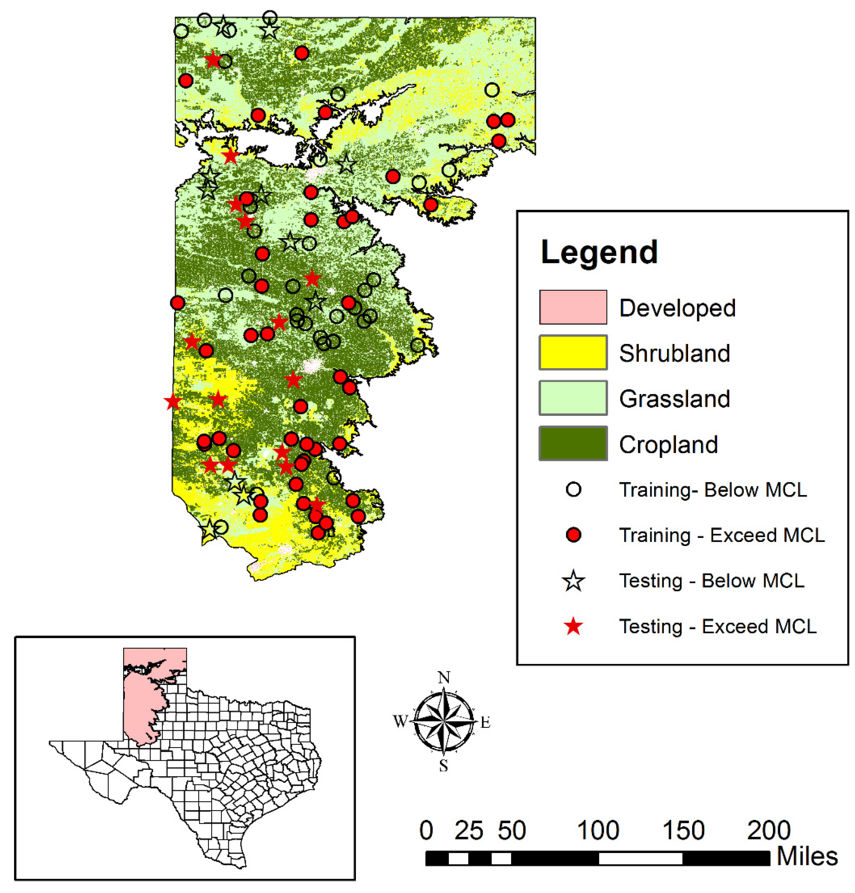
A comprehensive suite of potential input parameters was compiled from a variety of sources (see Table 1). Input values that were directly measured at the well (e.g., well depth, depth to water table and chemical constituents) were used directly. Other data (e.g., soil properties at the well) were extracted at the well using GIS operations. For modeling purposes, the entire dataset was randomly split into training (75 wells or 75%) and testing datasets (26 wells or 25%). The wells assigned to these datasets are depicted in Figure 1. All models were developed and coded using the R programming environment [69], making use of rpart [70], earth [71], randomforest [72] and dismo [73] packages and other custom developed scripts.
3. Results and Discussion
3.1. Model Development and Structural Inferences
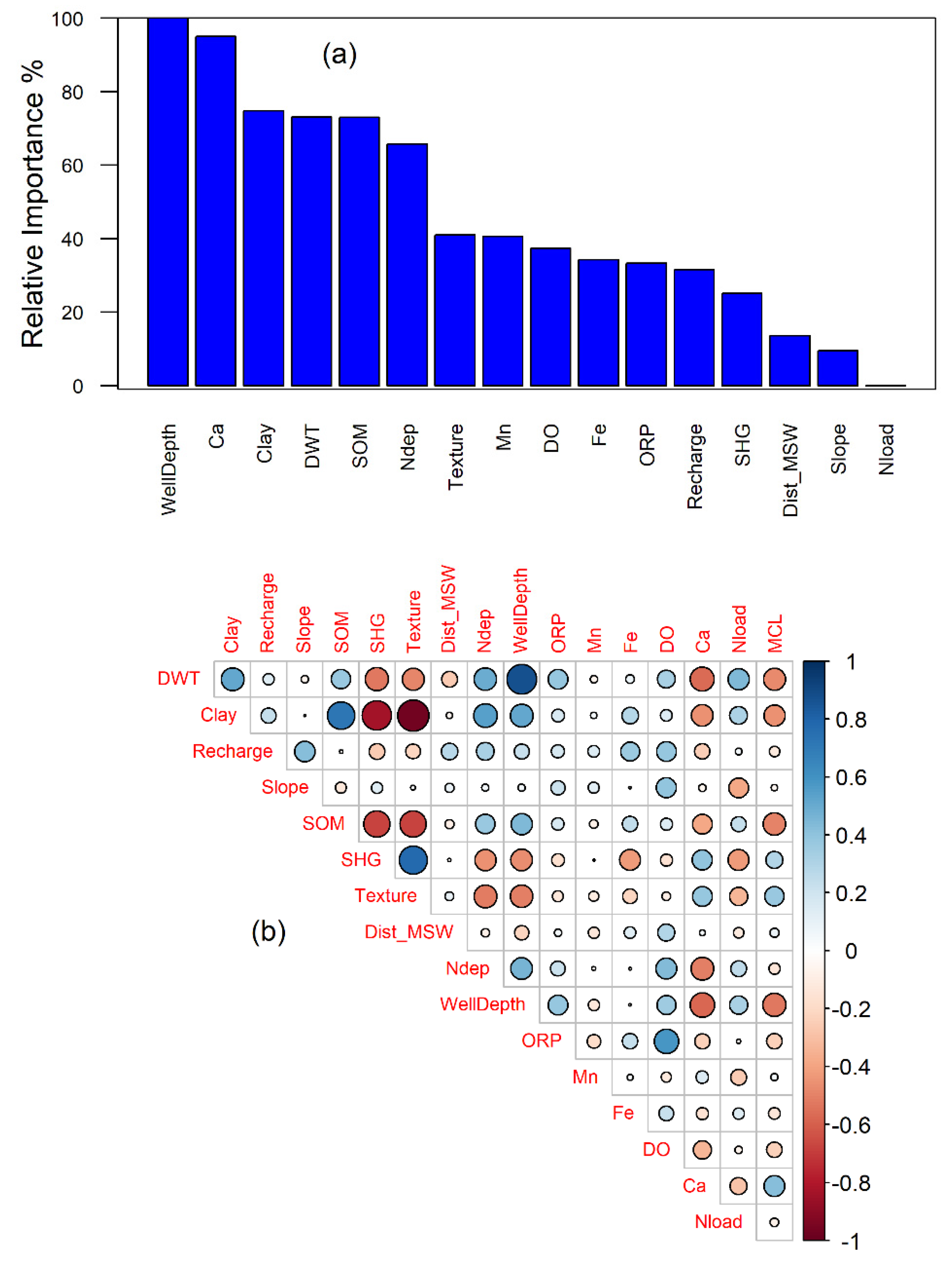
All models were calibrated using the training dataset (75 wells) and tested using the independent testing dataset (26 wells). The model coefficients for the logistic regression model are summarized in Table 2. The correlation coefficients and the relative importance computed using the filter-based feature selection method are depicted in Figure 2.
Four parameters—calcium concentration in the groundwater (Ca, mg/L), clay content of the overlying soil (clay, %), nitrogen deposition (Ndep-kg/ha/y) and Well Depth (WD in ft)—were selected due to their relative importance. While soil organic matter (SOM %) was also noted to be important, it exhibited a strong correlation with clay content, and as such was not included in the final model, to avoid multicollinearity effects. The model coefficients of the calibrated logistic regression model are presented in Table 2.
The Hosmer–Lemeshow test indicated no evidence of a poor fit (Chi-squared = 4.82, df = 8, p-value = 0.776) adding credence to the final selected model. The model coefficients for input parameters were statistically different from zero (α ≤ 0.05). The variance inflation factors were all less than 2.0 and as such the LR model did not exhibit any multicollinearity effects [74]. The model coefficients presented in Table 2 also indicate that the log-odds of an exceedance are inversely proportional to well depth and clay content. Deeper aquifers are oxygen depleted and higher clay content retards the free movement of air (oxygen) in the vadose zone, and thus minimizes oxygen availability as well.
Nitrogen deposition is also seen as an important predictor of nitrate exceedances. As nitrogen compounds have short residence times in the atmosphere [75], the deposition rates essentially serve as surrogates for local emission sources, such as releases from confined animal feed operations [76]. The SHP region is characterized by an abundance of calcite (caliche) deposits [77]. The dissolution of calcite in groundwater elevates the levels of calcium and carbonate in water. While calcium does not undergo significant reactions, the dissolution of bicarbonate increases the alkalinity. From stoichiometric considerations, the oxidation of 1 mg of ammonium-nitrogen to nitrate requires 7 mg of alkalinity; therefore, the dissolution of calcite promotes both the enrichment of calcium, as well as nitrate formation in the aquifer.
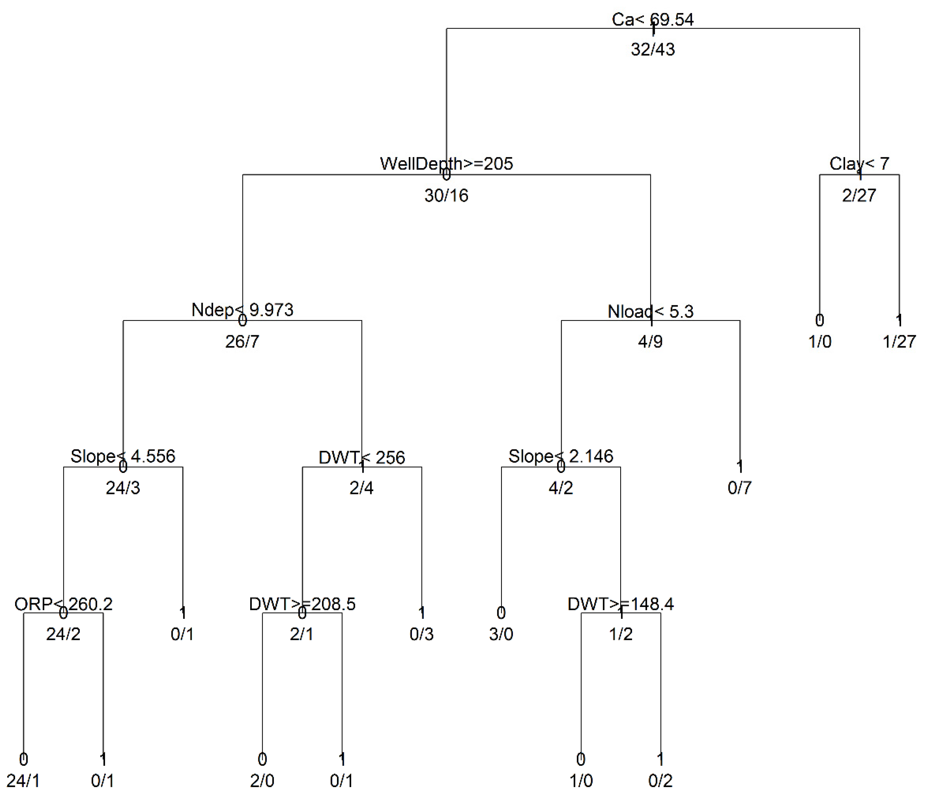
The final (pruned) CART model for the classification of nitrate exceedances in the Ogallala Aquifer is depicted in Figure 3. Higher level splits are performed using calcium, well depth, and clay percentage. The nitrogen deposition and nitrogen loading (a function of land use) have moderate influences, while depth to water table, slope and ORP have a lower level of influences. The final pruned CART model only used eight of the 16 inputs that were initially identified to likely influence the nitrate exceedances. The CART model variable selection (Figure 3) generally matches with the filter-based importance measures identified in Figure 2. Unlike LR models, which use a single global equation for prediction, CART models employ local models at each node, and as such are not affected by multicollinearity effects. Therefore, at lower level nodes (depth to water table which is strongly correlated to well depth), oxidation reduction potential (ORP, mV) tends to provide better splits on subsets of the data.
The final 10-fold cross-validated MARS model is summarized in Table 3. It uses four chemical parameters (calcium, ORP, nitrogen loading and nitrogen deposition), as well as two soil parameters (soil hydrologic group and clay); furthermore, the predictions also vary highly nonlinearly with well depth (as it is used for multiple cutoffs). Unlike the LR model, which was mostly based on intrinsic hydrogeological characteristics, the CART and MARS models placed a greater emphasis on geochemical processes. ORP is a direct indicator of redox processes in the aquifer. As deeper aquifers tend to exhibit anoxic or anerobic conditions, well depth can be viewed as a surrogate for redox processes in the aquifer. Therefore, the CART and MARS models emphasize that redox conditions in the aquifer play a critical role in defining nitrate concentrations. As discussed before, the selection of calcium to perform higher-order splits is consistent with the geochemical considerations, as it provides the alkalinity necessary for speciation of ammonium to nitrate ions.
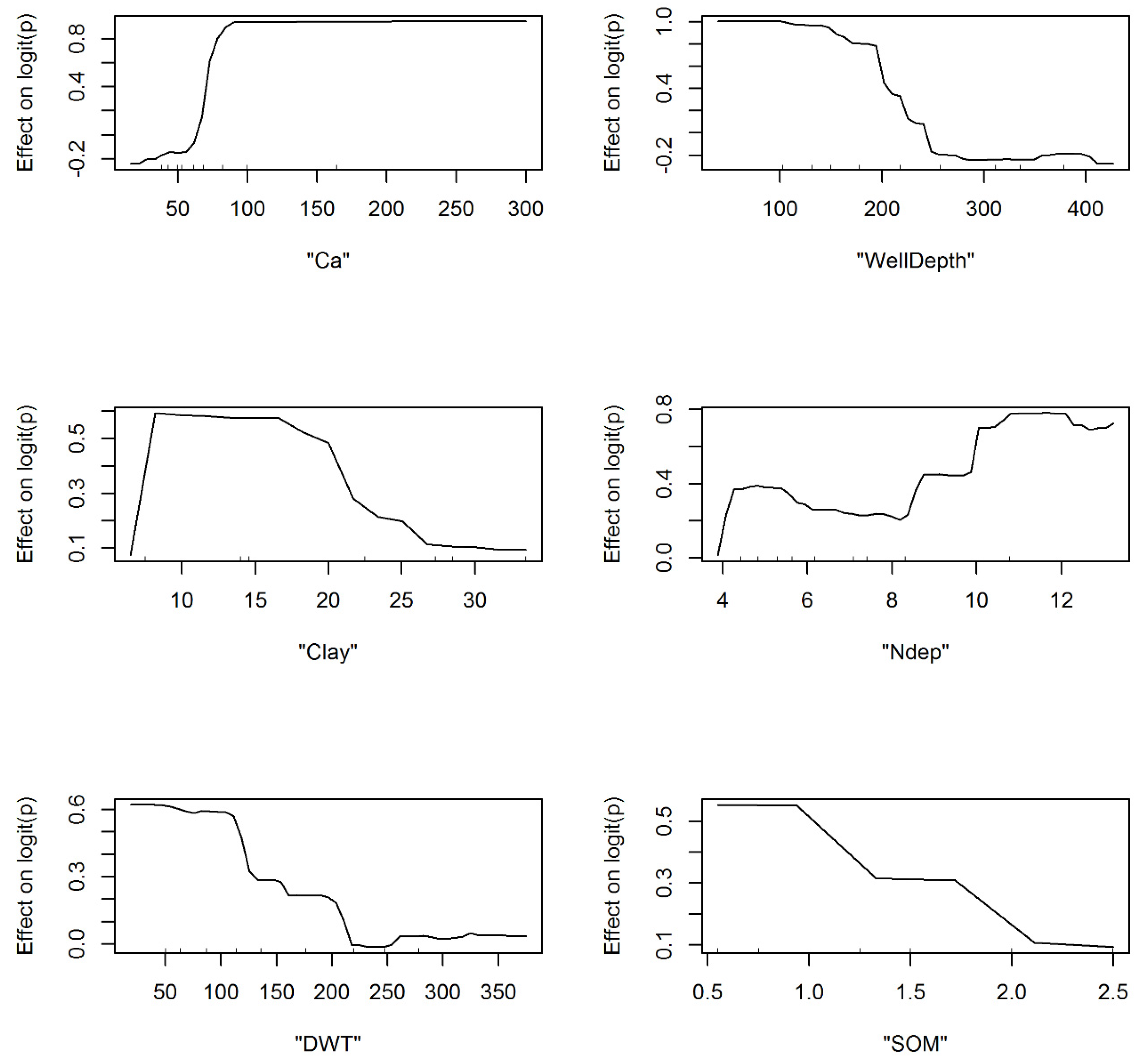
The random forest (RF) model was developed by optimizing the number of trees and the number of variables randomly sampled at each split. Cross-validation runs indicated that random sampling of four parameters yielded the best results. Additionally, the out of the bag (OOB) errors did not reduce significantly when the forest contained more than 2000 trees. The values obtained here for these hyper-parameters are consistent with other studies [78]. The RF algorithm is essentially a black-box model, with a focus on predictions rather than inferencing of the model structure. Nonetheless, important variables can be ascertained from random resampling of variables and the associated OOB errors. In addition, the marginal effects of input variables (i.e., the effect of a variable while controlling for others) on the logit can also be ascertained, and is depicted in Figure 4 for the six most important variables identified by the RF model.
In particular, the likelihood of predicting nitrate exceedances diminishes in wells that are deeper than 250 feet and when the depth to water table is greater than 200 ft. The exceedance of nitrate is also higher when the calcium concentrations in the well are greater than 100 mg/L. These results once again indicate the importance of aquifer redox chemistry for predicting nitrate exceedances and are generally consistent with CART and MARS model inferences.
The likelihood of nitrate exceedance is higher in areas with lower soil organic matter (typically indicative of agricultural lands) and decreases with increasing clay content (reduced recharge). The marginal effects of nitrate deposition indicate the likelihood of nitrate exceedance, which increases when annual loadings are greater than 8 kg-N/ha/y. The cyclical pattern of the marginal effects of nitrogen deposition (Ndep) in Figure 4 likely points to the interactions of this variable with other input parameters (i.e., effects are likely different depending upon the values of other inputs when calculating the marginals).
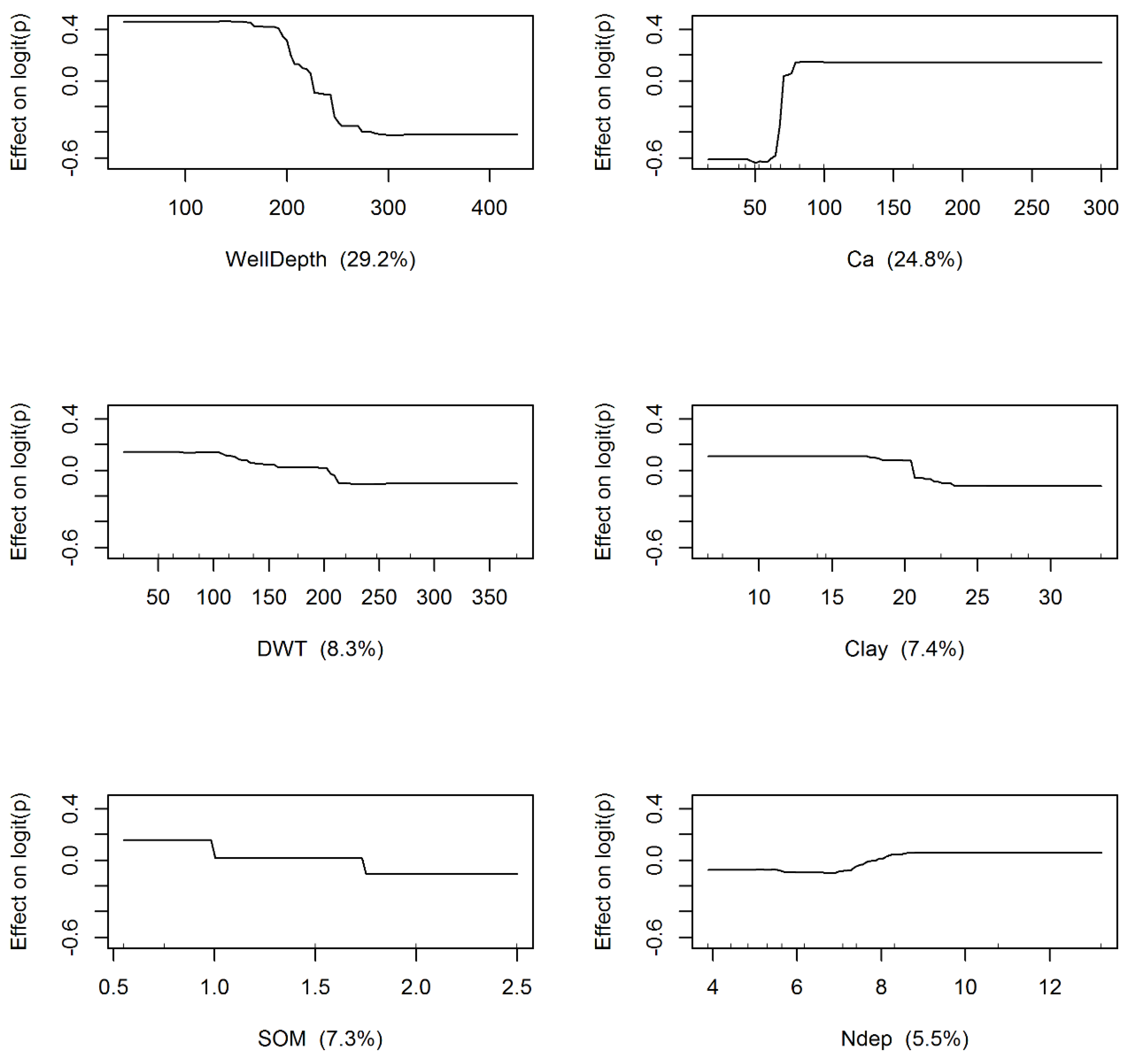
The calibration of gradient boosting algorithm (GBT) was carried out by jointly optimizing the number of trees (nt = 1290), learning rate (lr = 0.001) and tree complexity (tc = 5), using a 10-fold cross validation procedure [64]. Again, the gradient boosting places emphasis on prediction, rather than the inference of the underlying model structure. Nonetheless, the number of times a variable is selected for splitting and the associated improvement in prediction averaged over all trees can be used to identify significant variables [79]. Figure 5 shows the marginal effects of the six most important variables identified by the GBT model. The results in Figure 5 are similar to the partial dependencies obtained using the RF model. Again, the likelihood of observing nitrate exceedances decrease in wells with depths greater than 225 feet, and when the depth to the water table is greater than approximately 150 feet. Increasing clay content (>20%) and increasing soil organic matter (>1%) decrease the likelihood of observing nitrate exceedances. The GBT model also suggests that the likelihood of exceedance is higher when the total nitrogen deposition exceeds 8 kg-N/ha.
Elith et al. [64] have developed a procedure to assess interactions among variables, using trees developed as part of the model development process. The interactions calculated by establishing linear relationships between pairs of predictors while holding others at their average values indicate a strong relationship between nitrogen deposition (Ndep) and nitrate exceedances. As discussed earlier, nitrogen deposition is often considered a useful surrogate for local nitrogen sources in the region, such as the confined animal feed operations (CAFO).
3.2. Spatial Patterns of Controlling Factors
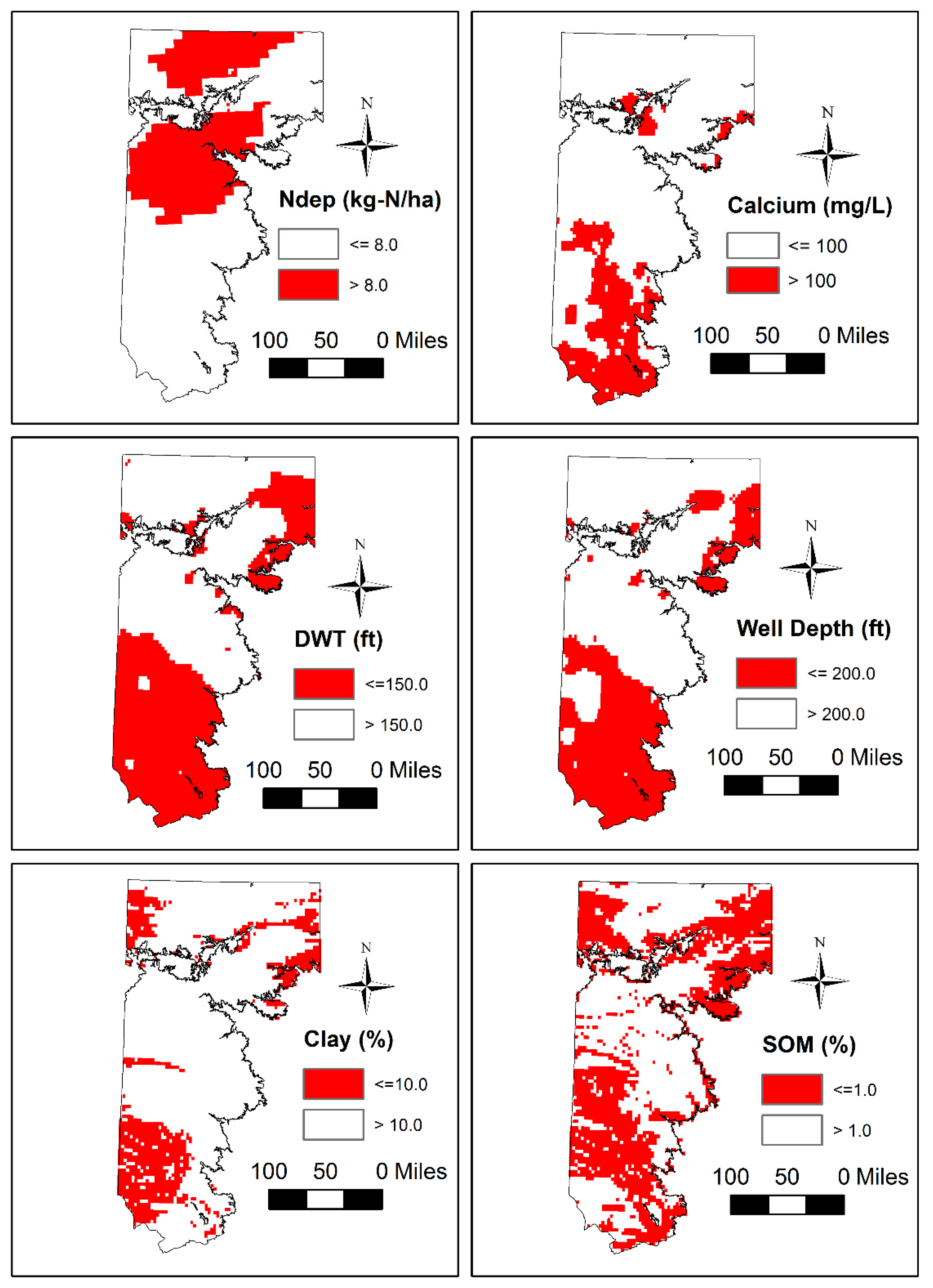
The insights generated from tree and ensemble-based modeling were integrated with GIS, to understand the spatial patterns of influencing variables, and are summarized in Figure 6.
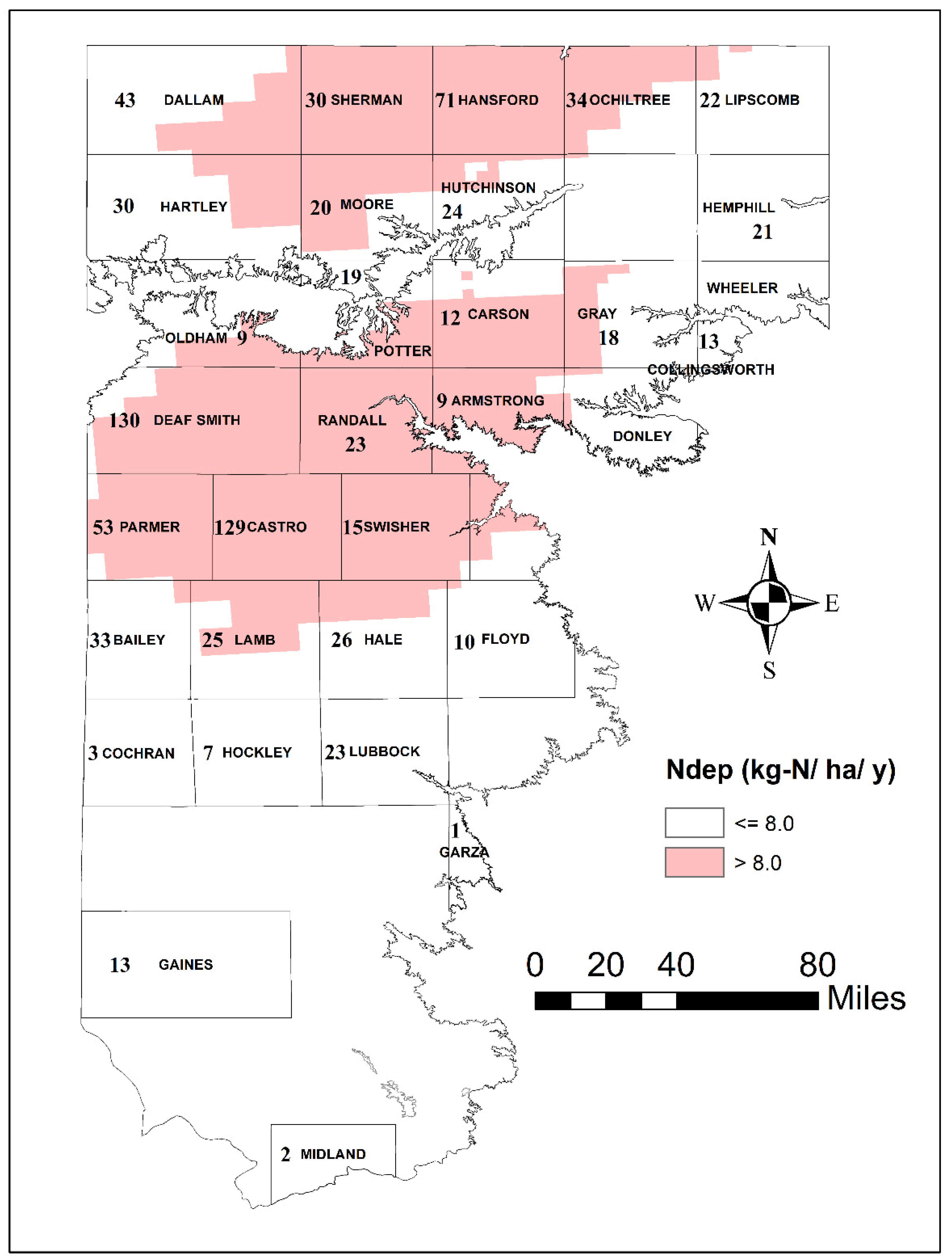
Nitrogen deposition in rural areas is a strong function of confined animal feed operations (CAFOs) [80], which are considered a significant source of ammonia emissions in West Texas [81]. There are a greater number of CAFOs in the northern portion of the study area (see Figure 7), which explains the greater influence of nitrogen deposition rate in the north.
The well depth and calcium, which are surrogates for redox reactions in the aquifer, are dominant in the southern portions of the study area. Furthermore, the depth to water table is significant in both the southern and northeastern sections. While the percentage of clay is selected as an important variable, its primary influence is seen mostly in the southwestern sections of the study area; however, this indicator correlates strongly with several other predictors (e.g., drainage, texture and soil organic matter (SOM)) used in the study. The soil organic matter (SOM) influence generally follows the agricultural land use in the region. These results, therefore, help conclude that CAFO operations and agriculture are likely the two dominant human activities that affect nitrogen in the Southern High Plains. Redox conditions in the aquifer play a significant role in controlling nitrate concentrations, especially in areas where the water table is shallow.
3.3. Predictive Evaluation of the Models
Separate contingency tables were created for each model for both training and testing datasets, using cut-off values obtained by simultaneously minimizing the distance to ideal sensitivity (recall) and specificity values of unity for each model (Table S1 in Supplementary Materials and Table 4 and Table 5). The null hypothesis that the observations and predictions are independent was rejected for both training and testing data, using Barnard’s exact test indicating the ability of the models to predict contamination states. A suite of summary measures was calculated for these contingency tables and are presented in Table 4 for training and Table 5 for testing datasets, to evaluate the predictive capabilities of the model. While the CART model is capable of being trained to a high level of accuracy, it is not able to sufficiently generalize the relationship and predict an independent dataset. Overfitting (i.e., the ability of a single tree to learn the training dataset well but unable to make generalizations) is known to be a problem with single tree models such as CART [82], and can be overcome using ensemble-based methods.
The performance of CART, MARS, and GBT are roughly similar over the suite of performance metrics evaluated. While the RF model performance is relatively low on the training dataset, it exhibits considerable generalization capabilities and does extremely well in predicting the independent testing dataset. The RF model has a high degree of accuracy, precision and recall, and relatively lower predictive errors for both positive (exceedance) and negative (non-exceedance) outcomes. Therefore, the RF model is capable of predicting both exceedances and non-exceedances with a high degree of accuracy. The Euclidian distance between the LR and tree-based models were calculated, to measure their relative performance to LR. Overall, RF performed significantly better, followed by GBT and MARS.
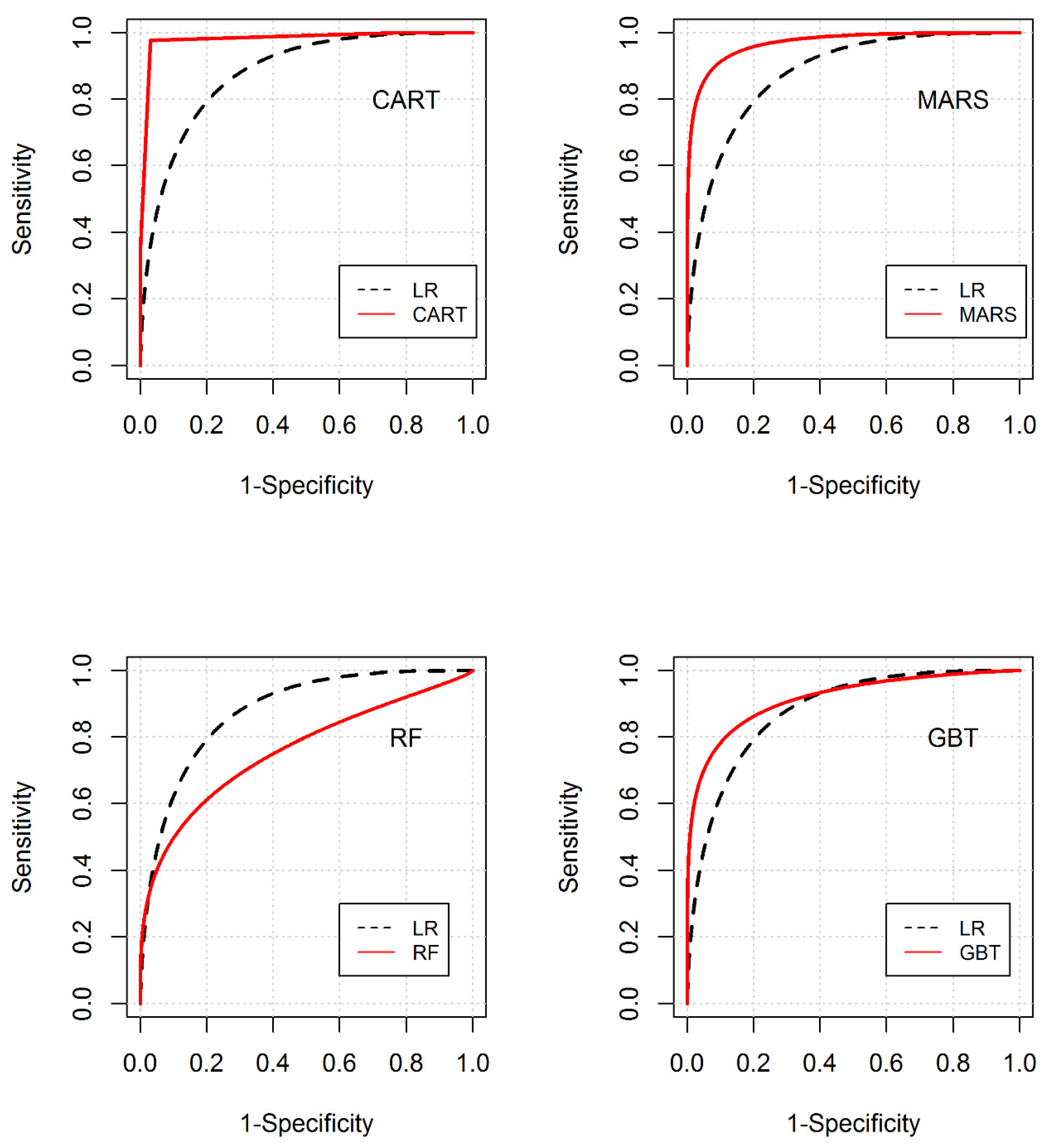
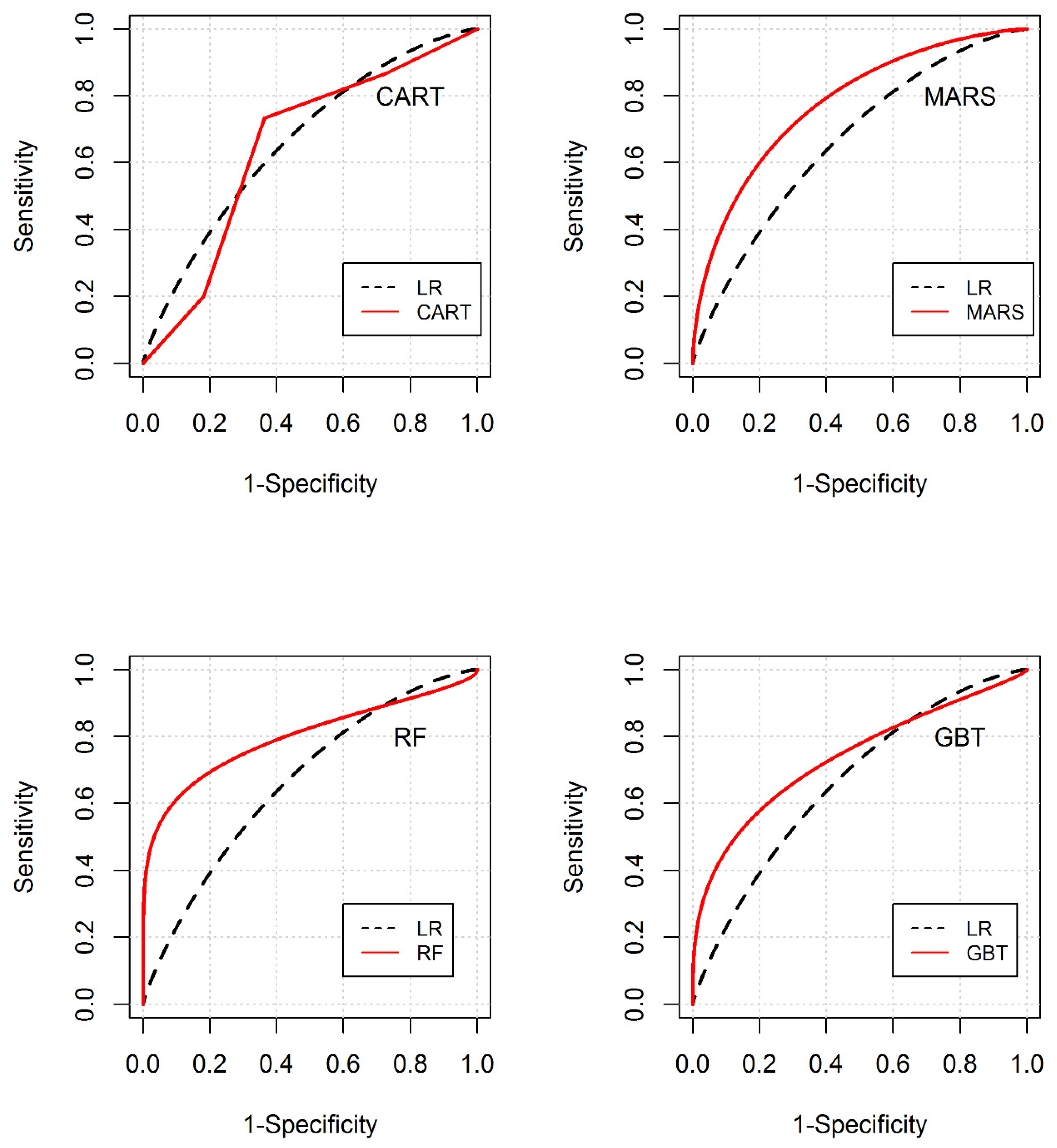
The receiver operating characteristics (ROC) curves were developed, to understand and compare the performance of the tree-based models against the LR model over the entire prediction spectrum. The results presented in Figure 8 for the training dataset indicate that the performances of CART and MARS models are slightly better than that of the LR over the entire range of specificity, while the GBT algorithm performs better for the lower values of specificity (i.e., 1-specificity > 0.5). A pair-wise bootstrap sampling test comparing the ROC curve for the LR model and these three tree-based models (CART, MARS and GBT) indicated that the differences were, however, statistically insignificant. The differences between the ROCs of LR and RF models were, however, significant (p < 0.001). The ROC plots (Figure 9) for the testing data also indicate that the performance of tree-based models is better over a large range of specificity, indicating their generally superior ability to predict exceedances in comparison to the LR model for the independent (testing) dataset.
3.4. Spatial Patterns of Aquifer Susceptibility to Nitrate Exceedances
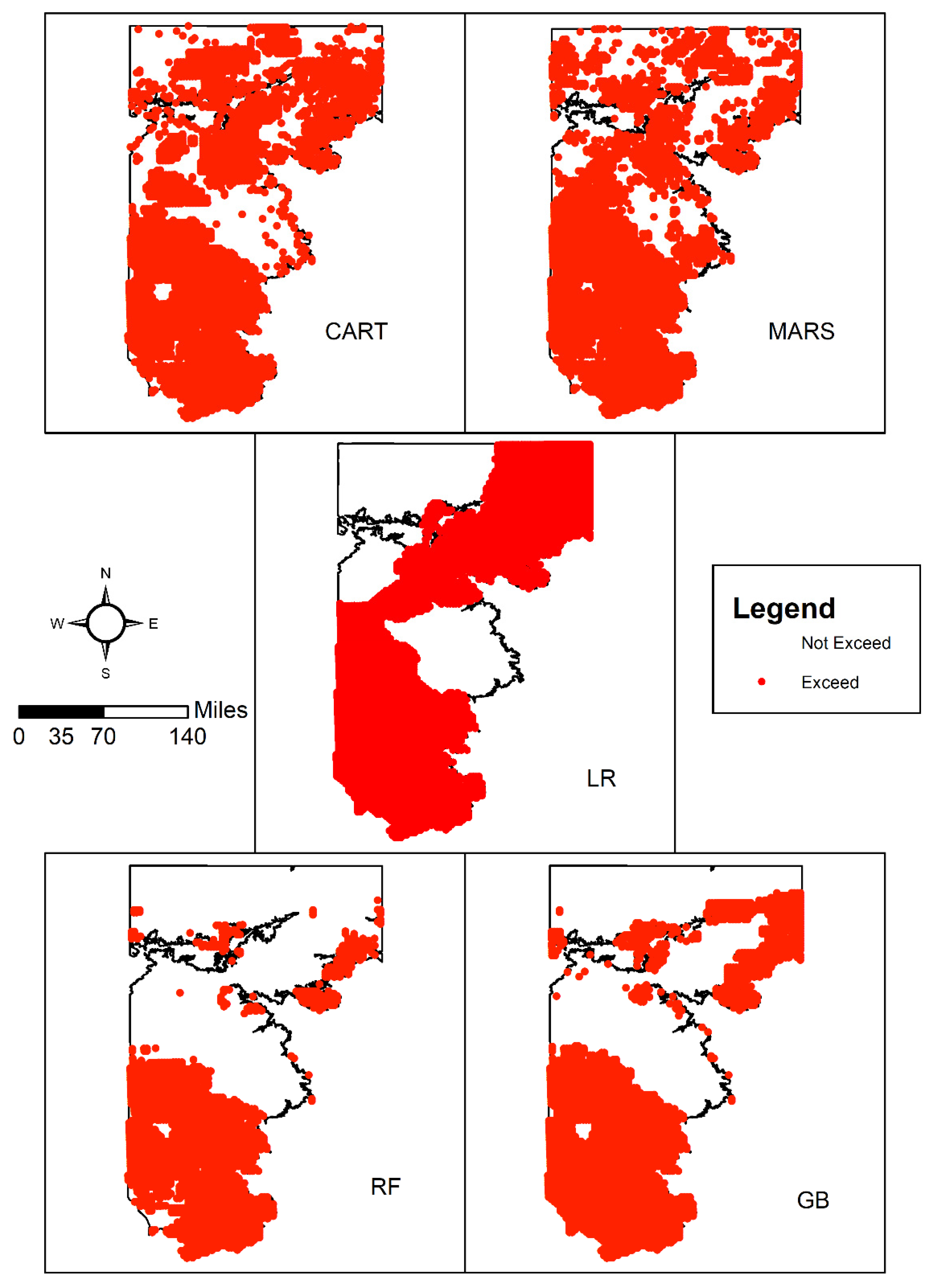
The five models developed as part of this study were applied to understand how predictions of nitrate vulnerability vary over the study area and across different techniques. For this purpose, the study area was gridded into 9196 equally spaced points (3 mile × 3 mile grid cells). The predictor values at each input was obtained using GIS and used in conjunction with the developed models to delineate aquifer vulnerability, and is depicted in Figure 10. All models predict high nitrate exceedances in the southern portions, as well as the northeastern edges of the aquifer. The Fleiss test indicated that there was a high degree of agreement between the models overall (p-value < 0.001). However, the models do vary the most in predicting vulnerability in the northwestern sections. The LR model was the most conservative and indicated that nearly 64.20% of the study area is susceptible to nitrate pollution. The CART and MARS models are less conservative and indicate that nearly 55% and 53% of the study area exhibit susceptibility to nitrate exceedances. The ensemble-based models were the least conservative of all techniques, with RF and GBT predicting that 32.76% and 43.45% of the study area were susceptible to nitrate exceedances. The output provided by these methods are smoother, with clearer distinctions between areas with exceedance and non-exceedance potential. The results here indicate that, while models may have statistically similar predictive behavior, their predictions can exhibit significant spatial variability.
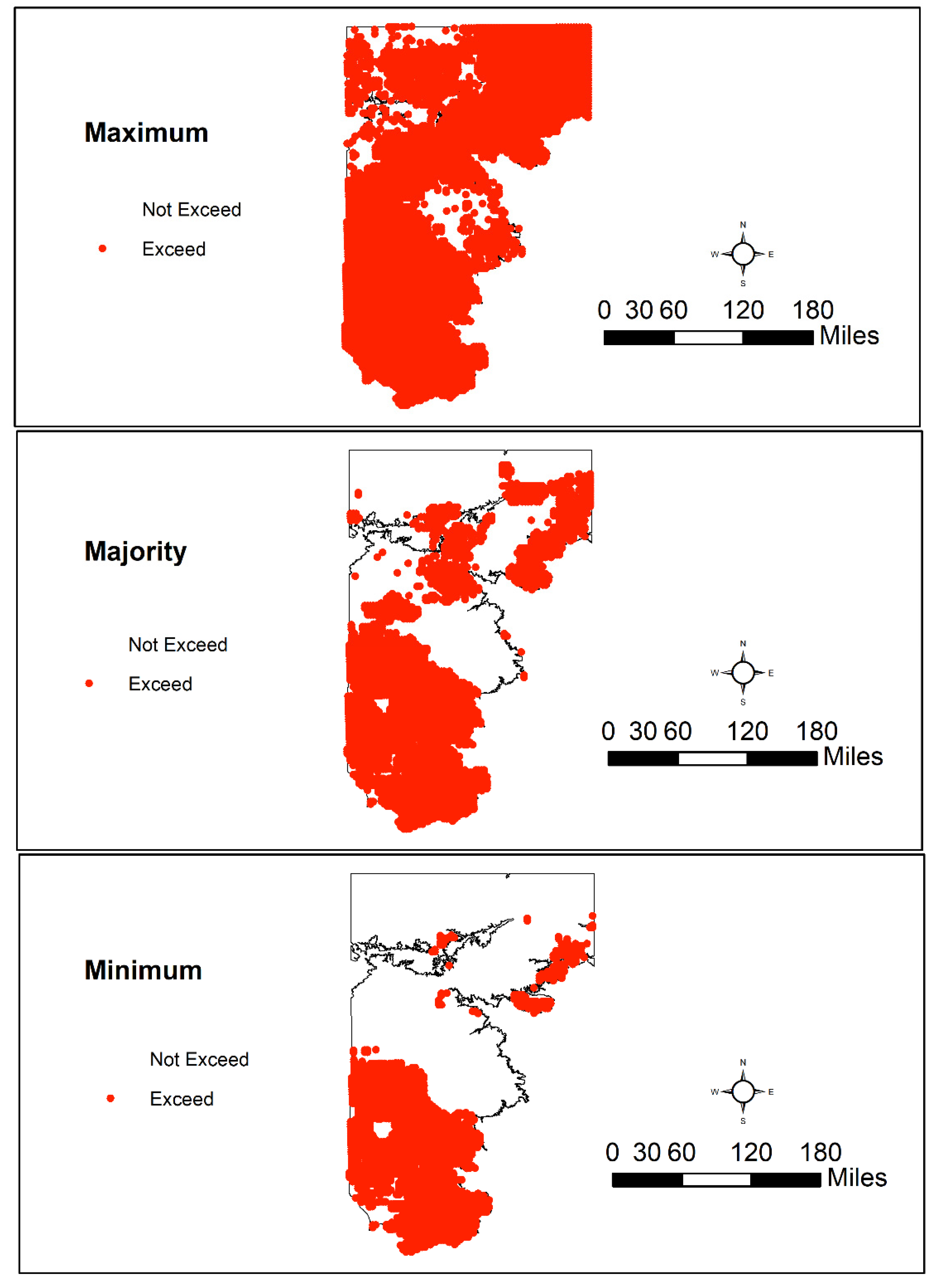
While the application of multiple models can be useful to generate scientific insights, results from these models pose challenges in practical regulatory applications. Many methods for the fusion of information generated from classifiers have been documented in the literature [83]. Here, the maximum, minimum and majority vote rules are adopted to develop composite maps for nitrate exceedance. The fusion based on maximum rule provides the most conservative depiction of aquifer vulnerability, in that a parcel is classified as vulnerable if at least one model classifies the model as being susceptible. On the other hand, the minimum rule is least conservative where the parcel of land is classified as not vulnerable, if at least one model categorizes the parcel as not being vulnerable. The majority rule classifies the parcel as vulnerable if a majority of the models (i.e., 3 or more) is in agreement with that assessment.
The results presented in Figure 11 indicate that the area identified as vulnerable in the “Minimum” map occupies 30% of the study area, and represents those locations that would require the greatest amount of characterization and sampling, as all five models categorize these parcels as being susceptible to nitrate exceedances, and all models categorize these parcels as being susceptible. The “Majority” map covers an additional 14% of the area to the vulnerable category and represents at least second priority sites, as three or more models classify them as likely being susceptible. The worst-case scenario is depicted by the “Maximum” map, which covers a little over 80% of the study area, or over 27,600 sq. miles. The area covered by the “Maximum” map, but not included in the “Majority” map, represents third priority areas for monitoring, as at least one of the models classifies it as being susceptible. It is, however, important to note that future monitoring must also include those areas that are not categorized as susceptible, albeit relatively less frequently, as the prioritization is based on present observations. Changes in land use and other hydrogeochemical conditions (e.g., water levels and ORP), which are relatively inexpensive to measure, can provide vital clues to initiate or ramp up nitrate monitoring activities.
4. Summary and Conclusions
Four different tree-based algorithms (i.e., CART, MARS, random forests (RF) and gradient noosting trees (GBT) were evaluated here to predict nitrate-nitrogen exceedances of drinking water standards in the Ogallala formation of the Southern High Plains (SHP) Aquifer in Texas. The algorithms of these tree-based models are useful to identify important variables necessary to model the output of interest. All four tree-based models highlight the important role of calcium dissolution in controlling the concentrations of nitrate in groundwater. Redox chemistry plays a critical role in quantifying the nitrate concentrations in groundwater. Indicators of redox, such as well depth, clay content in the soil and depth to water table, are also identified as being important. Soil organic matter (an indicator of agricultural activities) is also an important variable that correlates strongly with clay content of the soil. Nitrogen deposition rates were locally seen to be important and serve as a useful surrogate for potential releases from confined animal feed operations in the region. These variables were also noted to be important using the model-free feature selection method, adding credence to the abilities of the tree-based approaches to identify important parameters, and help elucidate underlying geochemical mechanisms controlling the fate and transport of nitrate in groundwater systems.
From a predictive standpoint, all tree-based models performed better than the logistic regression model, which provided the most conservative results. Tree-based models are able to refine the estimates locally, which LR models cannot do. Therefore, they are able to represent elevated nitrogen exposures in a better way than the LR model. Of the tree-based models, the random forest (RF) model exhibited the best generalization capabilities. While CART, MARS and GBT had similar accuracies, the MARS and GBT did slightly better in predicting exceedances, while the CART model as better at predicting non-exceedances. A short video summary of the framework and these major findings can also be found in the Supplementary Materials section (Video S1: videoabstract-TreeBasedNitrate,mp4) Based on the results from the study it can be concluded that tree-based models offer a transparent approach to modeling aquifer vulnerabilities and can be coupled with GIS to depict regional-scale aquifer vulnerability.
Supplementary Materials
The following are available online at https://www.mdpi.com/2073-4441/12/4/1023/s1, Table S1: Contingency Tables for Training and Testing Data for Various Models along with Cut-off Probabilities, Video S1: videoabstract-TreeBasedNitrate,mp4.
Author Contributions
Conceptualization, V.U. and E.A.H.; Data curation, A.L.B.S. and G.M.; Formal analysis, A.L.B.S. and S.S.; Funding acquisition, V.U.; Methodology, V.U.; Project administration, V.U. and S.S.; Supervision, V.U., E.A.H.; Validation, G.M. and E.A.H.; Visualization, A.L.B.S.; Writing—original draft, V.U.; Writing—review & editing, V.U., E.A.H. and G.M. All authors have read and agreed to the published version of the manuscript.
Funding
Partial support provided by the Ogallala Aquifer Program, an USDA-ARS led project including scientists from Kansas State University, Texas A&M AgriLife. Texas Tech University and West Texas A&M University, seeking solutions to problems arising from declining water availability from the Ogallala Aquifer (agreement number 58-3090-9-006).
Acknowledgments
Comments and suggestions from two anonymous reviewers is gratefully acknowledged. The support from Brazil Scientific Mobility Program to the second author (A.L.B.S) is noted with appreciation.
Conflicts of Interest
The authors declare no conflict of interest.
References
- WHO. Nitrite in Drinking-Water Background Document for Development of WHO Guidelines for Drinking-Water Quality; World Health Organization: Geneva, Switzerland, 2011; Available online: https://www.who.int/ (accessed on 19 February 2020).
- Pennino, M.; Compton, J.E.; Leibowitz, S.G. Trends in Drinking Water Nitrate Violations Across the United States. Environ. Sci. Technol. 2017, 51, 13450–13460. [Google Scholar] [CrossRef] [PubMed]
- United States Environmental Protection Agency. Available online: https://www.epa.gov/privatewells (accessed on 19 February 2020).
- DeSimone, L.A.; Hamilton, P.A.; Gilliom, R.J. Quality of ground water from private domestic wells. Water Well J. 2009, 63, 33–37. [Google Scholar]
- Gurdak, J.J.; Qi, S. Vulnerability of Recently Recharged Groundwater in Principle Aquifers of the United States to Nitrate Contamination. Environ. Sci. Technol. 2012, 46, 6004–6012. [Google Scholar] [CrossRef]
- Padilla, F.M.; Gallardo, M.; Manzano-Agugliaro, F. Global trends in nitrate leaching research in the 1960–2017 period. Sci. Total. Environ. 2018, 643, 400–413. [Google Scholar] [CrossRef] [PubMed]
- Wu, Y.; Liu, S. Impacts of biofuels production alternatives on water quantity and quality in the Iowa River Basin. Biomass Bioenergy 2012, 36, 182–191. [Google Scholar] [CrossRef]
- Gurdak, J.J.; Geyer, G.E.; Nanus, L.; Taniguchi, M.; Corona, C.R. Scale dependence of controls on groundwater vulnerability in the water–energy–food nexus, California Coastal Basin aquifer system. J. Hydrol. Reg. Stud. 2017, 11, 126–138. [Google Scholar] [CrossRef] [Green Version]
- Reddy, V.R.; Cunha, D.G.F.; Kurian, M. A Water–Energy–Food Nexus Perspective on the Challenge of Eutrophication. Water 2018, 10, 101. [Google Scholar] [CrossRef] [Green Version]
- King, A.; Jensen, V.; Fogg, G.; Harter, T. Groundwater remediation and management for nitrate. Tech. Rep. 2012, 5, 1–51. [Google Scholar]
- Keeler, B.L.; Polasky, S. Land-use change and costs to rural households: A case study in groundwater nitrate contamination. Environ. Res. Lett. 2014, 9, 074002. [Google Scholar] [CrossRef] [Green Version]
- Juntakut, P.; Haacker, E.M.K.; Snow, D.D.; Ray, A.C. Risk and Cost Assessment of Nitrate Contamination in Domestic Wells. Water 2020, 12, 428. [Google Scholar] [CrossRef] [Green Version]
- Lewandowski, A.; Montgomery, B.; Rosen, C.; Moncrief, J. Groundwater nitrate contamination costs: A survey of private well owners. J. Soil Water Conserv. 2008, 63, 153–161. [Google Scholar] [CrossRef]
- Aller, L.; Bennett, T.; Lehr, J.; Petty, R.; Hackett, G. DRASTIC: A Standardized System for Evaluating Ground Water Pollution Potential Using Hydrogeologic Settings; US Environmental Protection Agency: Washington, DC, USA, 1987.
- Uddameri, V.; Honnungar, V. Combining rough sets and GIS techniques to assess aquifer vulnerability characteristics in the semi-arid South Texas. Environ. Earth Sci. 2006, 51, 931–939. [Google Scholar] [CrossRef]
- Tesoriero, A.J.; Voss, F.D. Predicting the Probability of Elevated Nitrate Concentrations in the Puget Sound Basin: Implications for Aquifer Susceptibility and Vulnerability. Ground Water 1997, 35, 1029–1039. [Google Scholar] [CrossRef]
- Nolan, B.T.; Hitt, K.J.; Ruddy, B.C. Probability of Nitrate Contamination of Recently Recharged Groundwaters in the Conterminous United States. Environ. Sci. Technol. 2002, 36, 2138–2145. [Google Scholar] [CrossRef] [PubMed] [Green Version]
- Gardner, K.K.; Vogel, R.M. Predicting ground water nitrate concentration from land use. Ground Water 2005, 43, 343–352. [Google Scholar] [CrossRef] [PubMed] [Green Version]
- Liu, A.; Ming, J.; Ankumah, R.O. Nitrate contamination in private wells in rural Alabama, United States. Sci. Total. Environ. 2005, 346, 112–120. [Google Scholar] [CrossRef]
- Nolan, B.T.; Hitt, K.J. Vulnerability of Shallow Groundwater and Drinking-Water Wells to Nitrate in the United States. Environ. Sci. Technol. 2006, 40, 7834–7840. [Google Scholar] [CrossRef]
- Antonakos, A.; Lambrakis, N. Development and testing of three hybrid methods for the assessment of aquifer vulnerability to nitrates, based on the drastic model, an example from NE Korinthia, Greece. J. Hydrol. 2007, 333, 288–304. [Google Scholar] [CrossRef]
- Carbó, L.I.; Flores, M.C.; Herrero, M.A. Well site conditions associated with nitrate contamination in a multilayer semiconfined aquifer of Buenos Aires, Argentina. Environ. Earth Sci. 2008, 57, 1489–1500. [Google Scholar] [CrossRef]
- Warner, K.L.; Arnold, T. Relations that affect the probability and prediction of nitrate concentration in private wells in the glacial aquifer system in the United States. In Scientific Investigations Report; US Geological Survey: Reston, VA, USA, 2010. Available online: https://pubs.usgs.gov/sir/2010/5100/pdf/sir2010-5100.pdf (accessed on 19 February 2020).
- Venkataraman, K.; Uddameri, V. Modeling simultaneous exceedance of drinking-water standards of arsenic and nitrate in the Southern Ogallala aquifer using multinomial logistic regression. J. Hydrol. 2012, 458, 16–27. [Google Scholar] [CrossRef]
- Mair, A.; El-Kadi, A.I. Logistic regression modeling to assess groundwater vulnerability to contamination in Hawaii, USA. J. Contam. Hydrol. 2013, 153, 1–23. [Google Scholar] [CrossRef] [PubMed]
- Nolan, B.T.; Gronberg, J.M.; Faunt, C.C.; Eberts, S.M.; Belitz, K. Modeling Nitrate at Domestic and Public-Supply Well Depths in the Central Valley, California. Environ. Sci. Technol. 2014, 48, 5643–5651. [Google Scholar] [CrossRef]
- Rizeei, H.M.; Azeez, O.S.; Pradhan, B.; Khamees, H.H. Assessment of groundwater nitrate contamination hazard in a semi-arid region by using integrated parametric IPNOA and data-driven logistic regression models. Environ. Monit. Assess. 2018, 190, 633. [Google Scholar] [CrossRef] [PubMed]
- Gadbury, G.L.; Lyer, H.K.; Schreuder, H.T.; Ueng, C.Y. A nonparametric analysis of plot basal area growth using tree based models. In A Nonparametric Analysis of Plot Basal Area Growth Using Tree Based Models; U.S. Department of Agriculture-Forest Research Service: Fort Collins, CO, USA, 1997. Available online: https://www.fs.fed.us/rm/pubs/rmrs_rp002.pdf (accessed on 19 February 2020).
- McKenzie, N.; Ryan, P. Spatial prediction of soil properties using environmental correlation. Geoderma 1999, 89, 67–94. [Google Scholar] [CrossRef]
- Breiman, L.; Friedman, J.; Olshen, R.; Stone, C. Classification and Regression Trees; CRC Press: Boca Raton, FL, USA, 1984. [Google Scholar]
- Stidson, R.; Gray, C.A.; McPhail, C.D. Development and use of modelling techniques for real-time bathing water quality predictions. Water Environ. J. 2011, 26, 7–18. [Google Scholar] [CrossRef]
- Burow, K.R.; Nolan, B.T.; Rupert, M.G.; Dubrovsky, N.M. Nitrate in Groundwater of the United States, 1991−2003. Environ. Sci. Technol. 2010, 44, 4988–4997. [Google Scholar] [CrossRef]
- Friedman, J.H. Multivariate Adaptive Regression Splines. Ann. Stat. 1991, 19, 1–67. [Google Scholar] [CrossRef]
- Alonso-Fernández, J.R.; Nieto, P.G.; Muñiz, C.D.; Antón, J.C. Álvarez Modeling eutrophication and risk prevention in a reservoir in the Northwest of Spain by using multivariate adaptive regression splines analysis. Ecol. Eng. 2014, 68, 80–89. [Google Scholar] [CrossRef]
- Fortin, J.; Morais, A.; Anctil, F.; Parent, L. SVMLEACH—NK POTATO: A simple software tool to simulate nitrate and potassium co-leaching under potato crop. Comput. Electron. Agric. 2015, 110, 259–266. [Google Scholar] [CrossRef]
- Rezaie-Balf, M.; Naganna, S.; Ghaemi, A.; Deka, P.C. Wavelet coupled MARS and M5 Model Tree approaches for groundwater level forecasting. J. Hydrol. 2017, 553, 356–373. [Google Scholar] [CrossRef]
- Breiman, L. Random forests. Mach. Learn. 2001, 45, 5–32. [Google Scholar] [CrossRef] [Green Version]
- Breiman, L. Prediction games and arcing algorithms. Neural Comput. 1999, 11, 1493–1517. [Google Scholar] [CrossRef] [PubMed]
- Friedman, J.; Hastie, T.; Tibshirani, R. Additive logistic regression: A statistical view of boosting (With discussion and a rejoinder by the authors). Ann. Stat. 2000, 28, 337–407. [Google Scholar] [CrossRef]
- Ouedraogo, I.; Defourny, P.; Vanclooster, M. Modelling nitrate concentrations at the pan-African scale: A random forest approach. In Proceedings of the 1st Atlas Georesources International Congress (AGIC), Hammamet, Tunisia, 20–22 March 2017. [Google Scholar]
- Rodriguez-Galiano, V.; Mendes, M.P.; Garcia-Soldado, M.J.; Olmo, M.C.; Ribeiro, L. Predictive modeling of groundwater nitrate pollution using Random Forest and multisource variables related to intrinsic and specific vulnerability: A case study in an agricultural setting (Southern Spain). Sci. Total. Environ. 2014, 476, 189–206. [Google Scholar] [CrossRef] [PubMed]
- Nolan, B.T.; Fienen, M.; Lorenz, D.L. A statistical learning framework for groundwater nitrate models of the Central Valley, California, USA. J. Hydrol. 2015, 531, 902–911. [Google Scholar] [CrossRef] [Green Version]
- Hosseini, F.S.; Malekian, A.; Choubin, B.; Rahmati, O.; Cipullo, S.; Coulon, F.; Pradhan, B. A novel machine learning-based approach for the risk assessment of nitrate groundwater contamination. Sci. Total. Environ. 2018, 644, 954–962. [Google Scholar] [CrossRef] [Green Version]
- Crops and Plants [Online]. USDA-NASS: Washington, DC, USA, 2012. Available online: http://www.nass.usda.gov/ (accessed on 6 May 2013).
- Gurdak, J.J.; Qi, S. Vulnerability of recently recharged ground water in the High Plains aquifer to nitrate contamination. In Scientific Investigations Report; U.S. Geological Survey: Reston, VA, USA, 2006. Available online: https://pubs.usgs.gov/sir/2006/5050/ (accessed on 19 February 2020).
- Enwright, N.M.; Hudak, P.F. Spatial distribution of nitrate and related factors in the High Plains Aquifer, Texas. Environ. Earth Sci. 2009, 58, 1541–1548. [Google Scholar] [CrossRef]
- Scanlon, B.R.; Reedy, R.C.; Bronson, K.F. Impacts of Land Use Change on Nitrogen Cycling Archived in Semiarid Unsaturated Zone Nitrate Profiles, Southern High Plains, Texas. Environ. Sci. Technol. 2008, 42, 7566–7572. [Google Scholar] [CrossRef]
- Hamilton, J.D. State-space models. In Handbook of Econometrics IV; Elsevier: Amsterdam, The Netherlands, 1994. [Google Scholar]
- Smith, G. Step away from stepwise. J. Big Data 2018, 5, 32. [Google Scholar] [CrossRef]
- Saeys, Y.; Inza, I.; Larrañaga, P. A review of feature selection techniques in bioinformatics. Bioinformatics 2007, 23, 2507–2517. [Google Scholar] [CrossRef] [Green Version]
- Qian, S.S.; Anderson, C. Exploring Factors Controlling the Variability of Pesticide Concentrations in the Willamette River Basin Using Tree-Based Models. Environ. Sci. Technol. 1999, 33, 3332–3340. [Google Scholar] [CrossRef]
- Hancock, T.; Put, R.; Coomans, D.; Heyden, Y.V.; Everingham, Y. A performance comparison of modern statistical techniques for molecular descriptor selection and retention prediction in chromatographic QSRR studies. Chemom. Intell. Lab. Syst. 2005, 76, 185–196. [Google Scholar] [CrossRef]
- Clark, L.; Pregibon, D. Chapter Tree-Based Models. In Statistical Models in S; Chambers, J., Hastie, T., Eds.; CRC Press: Boca Raton, FL, USA, 1991. [Google Scholar]
- Leathwick, J.R.; Elith, J.; Hastie, T. Comparative performance of generalized additive models and multivariate adaptive regression splines for statistical modelling of species distributions. Ecol. Model. 2006, 199, 188–196. [Google Scholar] [CrossRef]
- Hastie, T.; Tibshirani, R. Discriminant Analysis by Gaussian Mixtures. J. R. Stat. Soc. Ser. B 1996, 58, 155–176. [Google Scholar] [CrossRef]
- Sutton, C.D. Classification and Regression Trees, Bagging, and Boosting. Handb. Stat. 2005, 24, 303–329. [Google Scholar]
- Breiman, L. Bias, Variance, and Arcing Classifiers; Tech. Rep. 460; Statistics Department, University of California: Berkeley, CA, USA, 1996. [Google Scholar]
- Breiman, L. Arcing classifier (with discussion and a rejoinder by the author). Ann. Stat. 1998, 26, 801–849. [Google Scholar] [CrossRef]
- Freund, Y.; Schapire, R.E. Experiments with a new boosting algorithm. icml 1996, 96, 148–156. [Google Scholar]
- Mason, L.; Baxter, J.; Bartlett, P.L.; Frean, M.R. Boosting algorithms as gradient descent. In Advances in Neural Information Processing Systems; MIT Press: Cambridge, MA, USA, 2000; pp. 512–518. Available online: https://papers.nips.cc/paper/1766-boosting-algorithms-as-gradient-descent.pdf (accessed on 19 February 2020).
- Hastie, T.; Tibshirani, R.; Friedman, J. Boosting and Additive Trees. In Springer Series in Statistics; Springer Science and Business Media LLC: Stanford, CA, USA, 2008; pp. 337–387. Available online: https://link.springer.com/chapter/10.1007%2F978-0-387-84858-7_10 (accessed on 19 February 2020).
- Schapire, R.E. The Boosting Approach to Machine Learning: An Overview. In Athens Conference on Applied Probability and Time Series Analysis; Springer Science and Business Media LLC: Florham Park, NJ, USA, 2003; Volume 171, pp. 149–171. Available online: https://link.springer.com/chapter/10.1007/978-0-387-21579-2_9 (accessed on 19 February 2020).
- Friedman, J.H. Greedy function approximation: A gradient boosting machine. Ann. Stat. 2001, 29, 1189–1232. [Google Scholar] [CrossRef]
- Elith, J.; Leathwick, J.R.; Hastie, T. A working guide to boosted regression trees. J. Anim. Ecol. 2008, 77, 802–813. [Google Scholar] [CrossRef]
- Friedman, J.H. Stochastic gradient boosting. Comput. Stat. Data Anal. 2002, 38, 367–378. [Google Scholar] [CrossRef]
- Agresti, A. An Introduction to Categorical Data Analysis; Wiley: Hoboken, NJ, USA, 2018. [Google Scholar]
- Fawcett, T. An introduction to ROC analysis. Pattern Recognit. Lett. 2006, 27, 861–874. [Google Scholar] [CrossRef]
- Burow, K.R.; Jurgens, B.C.; Belitz, K.; Dubrovsky, N.M. Assessment of regional change in nitrate concentrations in groundwater in the Central Valley, California, USA, 1950s–2000s. Environ. Earth Sci. 2012, 69, 2609–2621. [Google Scholar] [CrossRef]
- R Core Team. R: A Language and Environment for Statistical Computing; R Foundation for Statistical Computing: Vienna, Austria, 2019. [Google Scholar]
- Therneau, T.; Atkinson, B.; Ripley, B. Package ‘rpart’: Recursive Partitioning and Regression Trees. 2015, p. 34. Available online: https://cran.r-project.org/package=rpart (accessed on 19 February 2020).
- Milborrow, S. Package ‘earth’: Multivariate Adaptive Regression Splines. 2016, p. 51. Available online: http://www.milbo.users.sonic.net/earth (accessed on 19 February 2020).
- Liaw, A.; Wiener, M. Package ‘randomForest’: Breiman and Cutler’s Random Forests for Classification and Regression. 2015, p. 29. Available online: https://www.stat.berkeley.edu/~breiman/RandomForests/ (accessed on 19 February 2020).
- Hijmans, R.J.; Philips, S.; Leathwick, J.; Elith, J. Package ‘dismo’: Species Distribution Modeling. 2013, p. 68. Available online: http://rspatial.org/sdm/ (accessed on 19 February 2020).
- Midi, H.; Sarkar, S.; Rana, S. Collinearity diagnostics of binary logistic regression model. J. Interdiscip. Math. 2010, 13, 253–267. [Google Scholar] [CrossRef]
- Galloway, J.; Aber, J.D.; Erisman, J.W.; Seitzinger, S.; Howarth, R.W.; Cowling, E.B.; Cosby, B.J. The Nitrogen Cascade. Bioscience 2003, 53, 341. [Google Scholar] [CrossRef]
- Dayan, U.; Erel, Y.; Shpund, J.; Kordova, L.; Wanger, A.; Schauer, J.J. The impact of local sources and meteorological factors on nitrogen oxide and particulate matter concentrations: A case study of the Day of Atonement in Israel. Atmos. Environ. 2011, 45, 3325–3332. [Google Scholar] [CrossRef]
- Reeves, C.C. Origin, Classification, and Geologic History of Caliche on the Southern High Plains, Texas and Eastern New Mexico. J. Geol. 1970, 78, 352–362. [Google Scholar] [CrossRef]
- Peters, J.; De Baets, B.; Verhoest, N.E.C.; Samson, R.; Degroeve, S.; De Becker, P.; Huybrechts, W. Random forests as a tool for ecohydrological distribution modelling. Ecol. Model. 2007, 207, 304–318. [Google Scholar] [CrossRef]
- Friedman, J.H.; Meulman, J.J. Multiple additive regression trees with application in epidemiology. Stat. Med. 2003, 22, 1365–1381. [Google Scholar] [CrossRef]
- Costanza, J.K.; Marcinko, S.E.; Goewert, A.E.; Mitchell, C.E. Potential geographic distribution of atmospheric nitrogen deposition from intensive livestock production in North Carolina, USA. Sci. Total. Environ. 2008, 398, 76–86. [Google Scholar] [CrossRef]
- Rhoades, M.B.; Parker, D.B.; Cole, N.A.; Todd, R.W.; Caraway, E.A.; Auvermann, B.W.; Topliff, D.R.; Schuster, G.L. Continuous Ammonia Emission Measurements from a Commercial Beef Feedyard in Texas. Trans. ASABE 2010, 53, 1823–1831. [Google Scholar] [CrossRef]
- Qian, S.S. Environmental and Ecological Statistics with R, 2nd ed.; CRC Press Inc.: Boca, FL, USA, 2016. [Google Scholar]
- Kuncheva, L.; Bezdek, J.C.; Duin, R.P.W. Decision templates for multiple classifier fusion: An experimental comparison. Pattern Recognit. 2001, 34, 299–314. [Google Scholar] [CrossRef]
Figure 1.
Study Area and Locations of Nitrate Monitoring Wells.

Figure 2.
Relative Importance and Correlation Coefficient Matrix used for Selection of Inputs. (a) Relative Importance Measured using Filter-based Method and (b) Rank Correlation Coefficients between Variables (BiSerial Correlation was used for Discrete and Continuous Variable Correlations).
Figure 2.
Relative Importance and Correlation Coefficient Matrix used for Selection of Inputs. (a) Relative Importance Measured using Filter-based Method and (b) Rank Correlation Coefficients between Variables (BiSerial Correlation was used for Discrete and Continuous Variable Correlations).

Figure 3.
Classification and Regression Tree (CART) model for Nitrate Exceedances.

Figure 4.
Sensitivity of Salient Model Parameters and their Effect on Logit Computation in the Random Forest Model.
Figure 4.
Sensitivity of Salient Model Parameters and their Effect on Logit Computation in the Random Forest Model.

Figure 5.
Effects of Salient Model Parameters on Computed Logit for the Gradient Boosting Trees (GBT) Algorithm.
Figure 5.
Effects of Salient Model Parameters on Computed Logit for the Gradient Boosting Trees (GBT) Algorithm.

Figure 6.
Spatial Distribution of Salient Model Parameters Identified using Tree-Based Techniques.

Figure 7.
Number of Confined Animal Feed Lot Operations (CAFOs) in each County of the Study Area, along with Estimated Annual Nitrogen Deposition (Ndep).
Figure 7.
Number of Confined Animal Feed Lot Operations (CAFOs) in each County of the Study Area, along with Estimated Annual Nitrogen Deposition (Ndep).

Figure 8.
Comparison of Receiver Operating Characteristics (ROC) of Tree-Based and LR Model Classification for the Training Dataset.
Figure 8.
Comparison of Receiver Operating Characteristics (ROC) of Tree-Based and LR Model Classification for the Training Dataset.

Figure 9.
Receiver Operating Characteristics (ROC) Curves for Tree-Based Models in Comparison to the LR model.
Figure 9.
Receiver Operating Characteristics (ROC) Curves for Tree-Based Models in Comparison to the LR model.

Figure 10.
Prediction of Nitrate Exceedance across the Study Area by Different Methods.

Figure 11.
Nitrate Exceedances Mapping based on Different Model Aggregations (Minimum – all models are in agreement; Majority (most models are in agreement) and Maximum—at least one model predicts exceedance).
Figure 11.
Nitrate Exceedances Mapping based on Different Model Aggregations (Minimum – all models are in agreement; Majority (most models are in agreement) and Maximum—at least one model predicts exceedance).


Table 1.
Input Parameters Considered in this Study to Model Nitrate Exceedances and their Data Sources.
Table 1.
Input Parameters Considered in this Study to Model Nitrate Exceedances and their Data Sources.
| Parameter | Description | Source | Data Location |
|---|---|---|---|
| Recharge | Groundwater Recharge (in/yr) | 1% of 30-year Annual Precipitation from PRISM | http://www.prism.oregonstate.edu/normals/ (last access date: 19 February 2020) |
| Slope (%) | Topographical Slope (%) | Calculated using the 90 m Digital Elevation Map | http://srtm.csi.cgiar.org/ (last access date: 19 February 2020) |
| SOM | Soil Organic Matter (%) | STATSGO2 | http://websoilsurvey.sc.egov.usda.gov/App/HomePage.htm (last access date: 19 February 2020) |
| SHG | Soil Hydrologic Group | STATSGO2 | http://websoilsurvey.sc.egov.usda.gov/App/HomePage.htm (last access date: 19 February 2020) |
| Texture | Soil Texture | STATSGO2 | http://websoilsurvey.sc.egov.usda.gov/App/HomePage.htm (last access date: 19 February 2020) |
| Clay | Percent Clay (%) | STATSGO2 | http://websoilsurvey.sc.egov.usda.gov/App/HomePage.htm (last access date: 19 February 2020) |
| Dist_MSW | Distance from Muncipal Solid Waste Facility (mi) | Based on Locations identified by Texas Commission on Environmental Quality | https://www.tceq.texas.gov/permitting/waste_permits/msw_permits/msw-data (last access date: 19 February 2020) |
| Ndep | Nitrogen Deposition (kg/ha/y) | Based on National Atmospheric Deposition Program | http://nadp.slh.wisc.edu/NTN/maps.aspx (last access date: 19 February 2020) |
| DWT | Depth to Water Table (ft) | Texas Water Development Board Groundwater Database | http://www.twdb.texas.gov/groundwater/data/gwdbrpt.asp (last access date: 19 February 2020) |
| Well Depth | Well Depth (ft) | Texas Water Development Board Groundwater Database | http://www.twdb.texas.gov/groundwater/data/gwdbrpt.asp (last access date: 19 February 2020) |
| Mn | Manganese (mg/L) | Texas Water Development Board Groundwater Database | http://www.twdb.texas.gov/groundwater/data/gwdbrpt.asp (last access date: 19 February 2020) |
| Fe | Iron (mg/L) | Texas Water Development Board Groundwater Database | http://www.twdb.texas.gov/groundwater/data/gwdbrpt.asp (last access date: 19 February 2020) |
| Ca | Calcium (mg/L) | Texas Water Development Board Groundwater Database | http://www.twdb.texas.gov/groundwater/data/gwdbrpt.asp (last access date: 19 February 2020) |
| DO | Dissolved Oxygen (mg/L) | Texas Water Development Board Groundwater Database | http://www.twdb.texas.gov/groundwater/data/gwdbrpt.asp (last access date: 19 February 2020) |
| ORP | Oxidation Reduction potential (mV) | Texas Water Development Board Groundwater Database | http://www.twdb.texas.gov/groundwater/data/gwdbrpt.asp (last access date: 19 February 2020) |
| Nload | Nitrogen Loading (kg/y) | Based on land use land cover from MLRC 2011 | https://www.mrlc.gov/data/legends/national-land-cover-database-2011-nlcd2011-legend (last access date: 19 February 2020) |
Table 2.
Coefficients of the Logistic Regression (LR) Model (Standard Errors are in parenthesis).
| Parameter | Coefficient |
|---|---|
| (Intercept) | −0.189 (1.919) |
| Clay (%) | −0.0948 (0.044) |
| Ndep (kg/ha/y) | 0.454 (0.173) |
| WellDepth (ft) | −0.00955 (0.004) |
| Ca (mg/L) | 0.0248 (0.014) |
| AIC | 74.47 |
Table 3.
Model Coefficients of the MARS Model along with the Cut-Offs.
| Parameter | Coefficients |
|---|---|
| (Intercept) | 1.005 |
| h(SHG-8) | −0.436 |
| h(Clay-14) | −0.020 |
| h(Ndep-6.89954) | 0.109 |
| h(ORP-121.949) | 0.004 |
| h(96.9828-Ca) | −0.008 |
| h(Nload-7.5) | 0.115 |
| h(WellDepth-350) | −0.043 |
| h(WellDepth-190) | −0.005 |
| h(WellDepth-331) | 0.040 |
Table 4.
Performance Metrics of Tree-Based Models for the Training Dataset.
| Measure | Equation | LR | CART | MARS | RF | GBT |
|---|---|---|---|---|---|---|
| True Positive | TP | 35 | 42 | 41 | 28 | 36 |
| False Positive | FP | 6 | 1 | 2 | 7 | 3 |
| False Negative | FN | 8 | 1 | 2 | 15 | 7 |
| True Negative | TN | 26 | 31 | 30 | 25 | 29 |
| Prevalence | (TP + FN)/(TP+FP+FN+TN) | 0.573 | 0.573 | 0.573 | 0.573 | 0.573 |
| Accuracy | (TP+TN)/(TP+FP+FN+TN) | 0.813 | 0.973 | 0.947 | 0.707 | 0.867 |
| True Positive Rate | TP/(TP + FN) | 0.814 | 0.977 | 0.953 | 0.651 | 0.837 |
| False Positive Rate | FP/(TN + FP) | 0.188 | 0.031 | 0.063 | 0.219 | 0.094 |
| False Negative Rate | FN/(TP + FN) | 0.186 | 0.023 | 0.047 | 0.349 | 0.163 |
| True Negative Rate | TN/(TN + FP) | 0.813 | 0.969 | 0.938 | 0.781 | 0.906 |
| Positive Predictive Value | TP/(TP + FP) | 0.854 | 0.977 | 0.953 | 0.800 | 0.923 |
| False Omission Rate | FN/(TN + FN) | 0.235 | 0.031 | 0.063 | 0.375 | 0.194 |
| False Discovery Rate | FP/(TP + FP) | 0.146 | 0.023 | 0.047 | 0.200 | 0.077 |
| Negative Predictive Value | TN/(TN + FN) | 0.765 | 0.969 | 0.938 | 0.625 | 0.806 |
| Positive Likelihood Ratio | True Positive Rate/False Positive Rate | 4.341 | 31.256 | 15.256 | 2.977 | 8.930 |
| Negative Likelihood Ratio | False Negative Rate/ True Negative Rate | 0.229 | 0.024 | 0.050 | 0.447 | 0.180 |
| Diagnostic Odds Ratio | Positive Likelihood Ratio/Negative Likelihood Ratio | 18.958 | 1302.000 | 307.500 | 6.667 | 49.714 |
Table 5.
Performance Measures of Tree-Based Models for Testing Dataset.
| Measure | Equation | LR | CART | MARS | RF | GBT |
|---|---|---|---|---|---|---|
| True Positive | TP | 11 | 11 | 10 | 10 | 10 |
| False Positive | FP | 3 | 4 | 3 | 1 | 3 |
| False Negative | FN | 4 | 4 | 5 | 5 | 5 |
| True Negative | TN | 8 | 7 | 8 | 10 | 8 |
| Prevalence | (TP + FN)/(TP+FP+FN+TN) | 0.577 | 0.577 | 0.577 | 0.577 | 0.577 |
| Accuracy | (TP+TN)/(TP+FP+FN+TN) | 0.577 | 0.692 | 0.692 | 0.769 | 0.692 |
| True Positive Rate | TP/(TP + FN) | 0.667 | 0.733 | 0.667 | 0.667 | 0.667 |
| False Positive Rate | FP/(TN + FP) | 0.545 | 0.364 | 0.273 | 0.091 | 0.273 |
| False Negative Rate | FN/(TP + FN) | 0.333 | 0.267 | 0.333 | 0.333 | 0.333 |
| True Negative Rate | TN/(TN + FP) | 0.455 | 0.636 | 0.727 | 0.909 | 0.727 |
| Positive Predictive Value | TP/(TP + FP) | 0.625 | 0.733 | 0.769 | 0.909 | 0.769 |
| False Omission Rate | FN/(TN + FN) | 0.500 | 0.364 | 0.385 | 0.333 | 0.385 |
| False Discovery Rate | FP/(TP + FP) | 0.375 | 0.267 | 0.231 | 0.091 | 0.231 |
| Negative Predictive Value | TN/(TN + FN) | 0.500 | 0.636 | 0.615 | 0.667 | 0.615 |
| Positive Likelihood Ratio | True Positive Rate/False Positive Rate | 1.222 | 2.017 | 2.444 | 7.333 | 2.444 |
| Negative Likelihood Ratio | False Negative Rate/ True Negative Rate | 0.733 | 0.419 | 0.458 | 0.367 | 0.458 |
| Diagnostic Odds Ratio | Positive Likelihood Ratio/Negative Likelihood Ratio | 1.667 | 4.813 | 5.333 | 20.000 | 5.333 |
© 2020 by the authors. Licensee MDPI, Basel, Switzerland. This article is an open access article distributed under the terms and conditions of the Creative Commons Attribution (CC BY) license (http://creativecommons.org/licenses/by/4.0/).
Share and Cite
MDPI and ACS Style
Uddameri, V.; Silva, A.L.B.; Singaraju, S.; Mohammadi, G.; Hernandez, E.A. Tree-Based Modeling Methods to Predict Nitrate Exceedances in the Ogallala Aquifer in Texas. Water 2020, 12, 1023. https://doi.org/10.3390/w12041023
AMA Style
Uddameri V, Silva ALB, Singaraju S, Mohammadi G, Hernandez EA. Tree-Based Modeling Methods to Predict Nitrate Exceedances in the Ogallala Aquifer in Texas. Water. 2020; 12(4):1023. https://doi.org/10.3390/w12041023
Chicago/Turabian StyleUddameri, Venkatesh, Ana Luiza Bessa Silva, Sreeram Singaraju, Ghazal Mohammadi, and E. Annette Hernandez. 2020. "Tree-Based Modeling Methods to Predict Nitrate Exceedances in the Ogallala Aquifer in Texas" Water 12, no. 4: 1023. https://doi.org/10.3390/w12041023
Note that from the first issue of 2016, this journal uses article numbers instead of page numbers. See further details here.