Article

Influence of Farming Intensity and Climate on Lowland Stream Nitrogen

1
Departamento de Ecología y Gestión Ambiental, Centro Universitario Regional Este (CURE), Universidad de la República, Punta del Este 20100, Uruguay
2
Department Aquatic Ecosystem Analysis, Helmholtz Centre for Environmental Research—UFZ, 39114 Magdeburg, Germany
3
Department of Bioscience and Arctic Research Centre, Aarhus University, 8600 Silkeborg, Denmark
4
Sino-Danish Centre for Education and Research, Beijing 100000, China
5
Limnology Laboratory, Department of Biological Sciences and EKOSAM, Middle East Technical University, 06800 Ankara, Turkey
6
Leibniz-Institute of Freshwater Ecology and Inland Fisheries, 12587 Berlin, Germany
7
South American Institute for Resilience and Sustainability Studies (SARAS), Bella Vista 20302, Uruguay
*
Author to whom correspondence should be addressed.
Water 2020, 12(4), 1021; https://doi.org/10.3390/w12041021
Submission received: 17 February 2020 / Revised: 19 March 2020 / Accepted: 30 March 2020 / Published: 2 April 2020
(This article belongs to the Special Issue Land Use and Water Quality)

Abstract

:
Nitrogen lost from agriculture has altered the geochemistry of the biosphere, with pronounced impacts on aquatic ecosystems. We aim to elucidate the patterns and driving factors behind the N fluxes in lowland stream ecosystems differing about land-use and climatic-hydrological conditions. The climate-hydrology areas represented humid cold temperate/stable discharge conditions, and humid subtropical climate/flashy conditions. Three complementary monitoring sampling characteristics were selected, including a total of 43 streams under contrasting farming intensities. Farming intensity determined total dissolved N (TDN), nitrate concentrations, and total N concentration and loss to streams, despite differences in soil and climatic-hydrological conditions between and within regions. However, ammonium (NH4+) and dissolved organic N concentrations did not show significant responses to the farming intensity or climatic/hydrological conditions. A high dissolved inorganic N to TDN ratio was associated with the temperate climate and high base flow conditions, but not with farming intensity. In the absence of a significant increase in farming N use efficiency (or the introduction of other palliative measures), the expected farming intensification would result in a stronger increase in NO3, TDN, and TN concentrations as well as in rising flow-weighted concentrations and loss in temperate and subtropical streams, which will further exacerbate eutrophication.

1. Introduction

The changes promoted by agriculture in terrestrial and freshwater ecosystems can be quite dramatic [1,2]. During the 20th and 21st centuries, the global nitrogen (N) cycle has accelerated due to the artificial fixation of atmospheric N2 (g) and extensive use of N fertilizers to boost agricultural production [3,4]. A high amount of reactive N (~100 Tg N·year−1) is used in global agriculture, but it is estimated that less than 1 out of every 5 N-atoms used as fertilizer is finally consumed by humans [3]. The N lost from agricultural production ultimately alters the geochemistry of the biosphere and particularly impacts aquatic ecosystems, thus contributing to eutrophication, degradation of water quality, and biodiversity loss [5,6,7,8,9].
At the catchment scale, the biogeochemical processes determining the natural fluxes of N from land to aquatic ecosystems mainly depend on climatic and hydrological regimes, and their interaction with local soil and geological conditions [10]. Consequently, stream N concentrations are dependent on variations in water temperature and discharge [11,12,13]. Moreover, farming intensity alters N mass balance and fluxes, leading to changes in the hydrochemistry of the streams [14]. One of the main changes induced by agriculture is the enhanced N level [4] due to the higher input of dissolved inorganic N (DIN), resulting in increased nitrate exports to aquatic ecosystems [15,16].
Intensive farming is a worldwide phenomenon [1,17]. Europe has a much longer history of intensive farming than tropics and subtropics, where the expansion of cropland areas became particularly rapid after 1850 [18]. Furthermore, 50% of the N fertilizer (inorganic and manure) used is confined to approximately 10% of the fertilized land, in tropical and subtropical areas of south and southeast Asia and southeast South America [19,20]. So far, most studies of the environmental consequences of N use in farming on streams have been conducted in developed countries, particularly in areas characterized by a temperate climate within Europe and North America [21], whereas only a few investigations have focused on developing countries and/or warm climate conditions e.g., [22,23,24]. Better knowledge of the use, transformation, and transport of N in subtropical and tropical climate regions—and thus of the N cycle—is urgently needed to generate more nutrient-efficient ways of producing food, while simultaneously reducing the negative side effects on the environment [18,25,26,27].
We aim to elucidate the patterns and driving factors behind the N fluxes in lowland stream ecosystems with contrasting land-uses and climate. Specifically, we aimed to analyze to what extent natural variations in soil characteristics and climate/hydrology would influence the effect of catchment farming on concentrations and N losses in lowland streams. We expected that streams draining microcatchments with high-intensity farming would have the highest concentrations of total N (TN), total dissolved N (TDN), nitrate (NO3), ammonium (NH4+), and dissolved organic N (DON) and a higher DIN/TDN ratio than streams draining low-intensity farming microcatchments, independently of variations in edaphic variability or climatic-hydrological conditions.

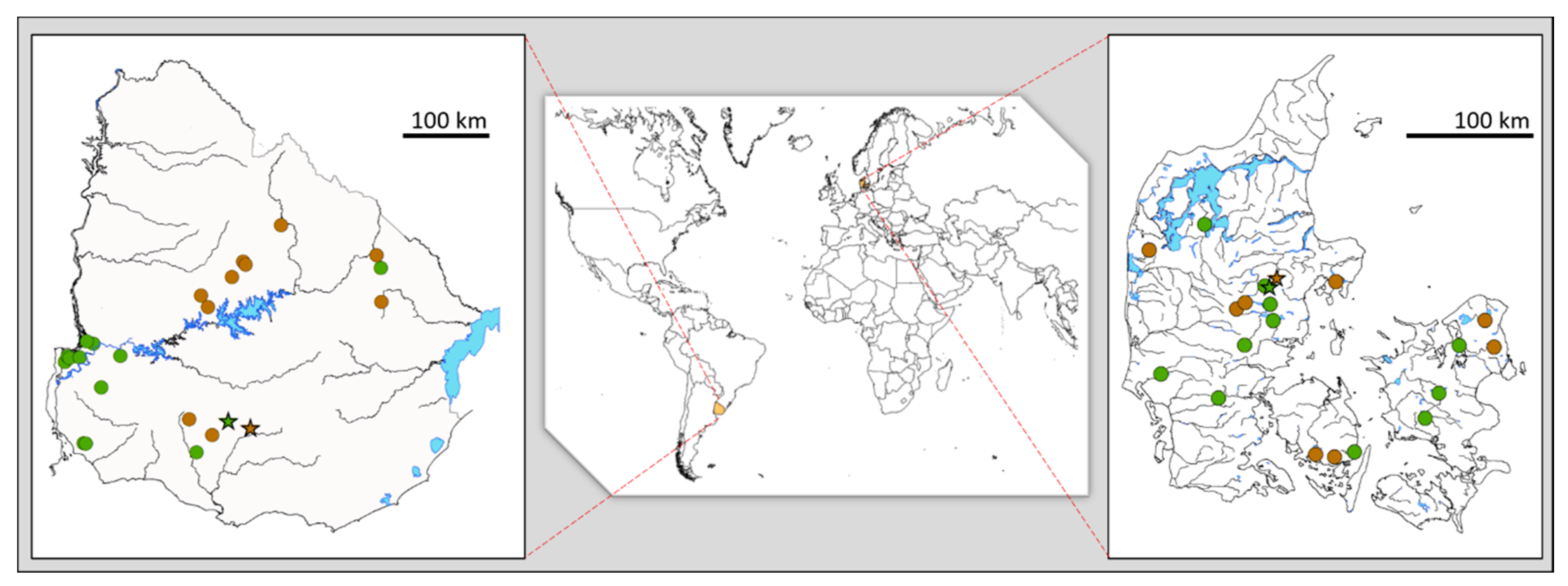
2. Materials and Methods

To obtain a suitable balance between the different scales of analysis [28], the sampling strategy included three complementary monitoring schemes using different combinations of sampling frequencies and the associated number of streams (considered as replicates of farming intensity within each region).
A total of 43 lowland streams draining microcatchments under two contrasting conditions of agricultural intensity (hereafter farming intensity) were selected in two distinctive climate areas: humid cold temperate (Dfb sensu: [29]; n = 21 in summer; n = 20 in winter) and humid subtropical (Cfa sensu: [29]; n = 22; Table 1). The topography of both selected landscapes was characterized by gently rolling plains (mean slope < 5%) and the hydrographic catchment size varied around 10 km2 (Denmark 9 ± 11 km2, Uruguay 12 ± 7 km2, average and standard deviation, respectively).
One stream per combination of farming intensity/climate-hydrology condition (nstreams = 4, Table 1) was described in detail relative to hydrology, hydrochemistry, meteorological conditions, and catchment land-use. These streams acted as “benchmark streams” for each condition, and water samples with two different temporal resolutions were taken for a 2-year period (see Section 2.2). Both Danish benchmark streams are part of the Gudenå River basin, while the Uruguayan benchmark streams are part of the Santa Lucía Chico River basin. Besides the benchmark streams, a larger set of streams grouped according to farming intensity/climate-hydrology conditions were sampled with a “snapshot” approach (nstreams = 39 winter, 38 summer; 1 sample per season; Table 1). More detailed information can be found in Goyenola et al. [30] and Graeber et al. [31]. Automatized gauging stations were established in the four benchmark microcatchments. Hydrometric data were recorded every 10 minutes using CR10X data loggers (Campbell Scientific Ltd., Shepshed, UK). In the subtropical streams, we used CS450 Submersible Pressure Transducers (Campbell Scientific Ltd., Shepshed, UK) for water stage monitoring and Rain-O-Matic Professional rainfall automatized gauges (Pronamic). In temperate catchments, the water level was registered with PDCR 1830 pressure sensors (Druck), while meteorological information was obtained from the Danish Meteorological Institute monitoring the network based on a 10 × 10 km grid. Periodic instantaneous flow measurements were taken using a C2-OTT Kleinflügel, transferring data to software for the calculation of instantaneous discharge (VB-Vinge 3.0, Mølgaard Hydrometri).
Nitrogen catchment input by hectare and year in Danish catchments was estimated considering the surface of agriculture land in the catchment multiplied by the national average of chemical fertilizer use for the years 2011–2012 (total input 69 kg N·ha−1·year−1), and the livestock density multiplied by the average of N production in manure by livestock (86 kg N·ha−1·year−1 [32]). Nitrogen catchment input by hectare and year in Uruguayan catchments was estimated through interviews with the technical managers of the establishments. Based on the best available knowledge considering empirical data [33], the average of N production in manure for the Uruguayan was assumed to equal than for Danish catchments. The total N input was divided by the total catchment area to be able to make quantitative comparisons with the TN losses.

2.1. Farming Intensity

Land-use intensity is a complex multidimensional concept and is difficult to measure [34,35], and therefore we applied explicit operational definitions (Table 1). Low-intensity farming catchments represent the condition with minimal anthropogenic pressures for each region. The subtropical low-intensity farming catchments (n = 9, both summer and winter) were dominated by the natural grasslands of the Pampa Biome [36] and sustained low-density cattle production (below one head per hectare), while a mixture of deciduous and coniferous forests dominated the temperate low-intensity farming catchments (nsummer = 8; nwinter = 9; Figure 1; Table 1). Less than 30% of the selected low-intensity farming catchments in both countries were influenced by arable cropping systems.
The criteria for the selection of high-intensity farming catchments were: (1) that arable cropping systems with intensive use of fertilizers affected more than 70% of the total area and (2) that they represented real and typical high-intensity farming catchments in the climatic-hydrological regions of the two countries (nTEMP = 12; nSUBT = 13; Table 1).

2.2. Hydrochemistry Monitoring

The complementary strategy allowed us to evaluate whether the patterns observed were generalizable for each climate/hydrological region or even common to both. The monitoring approach included:
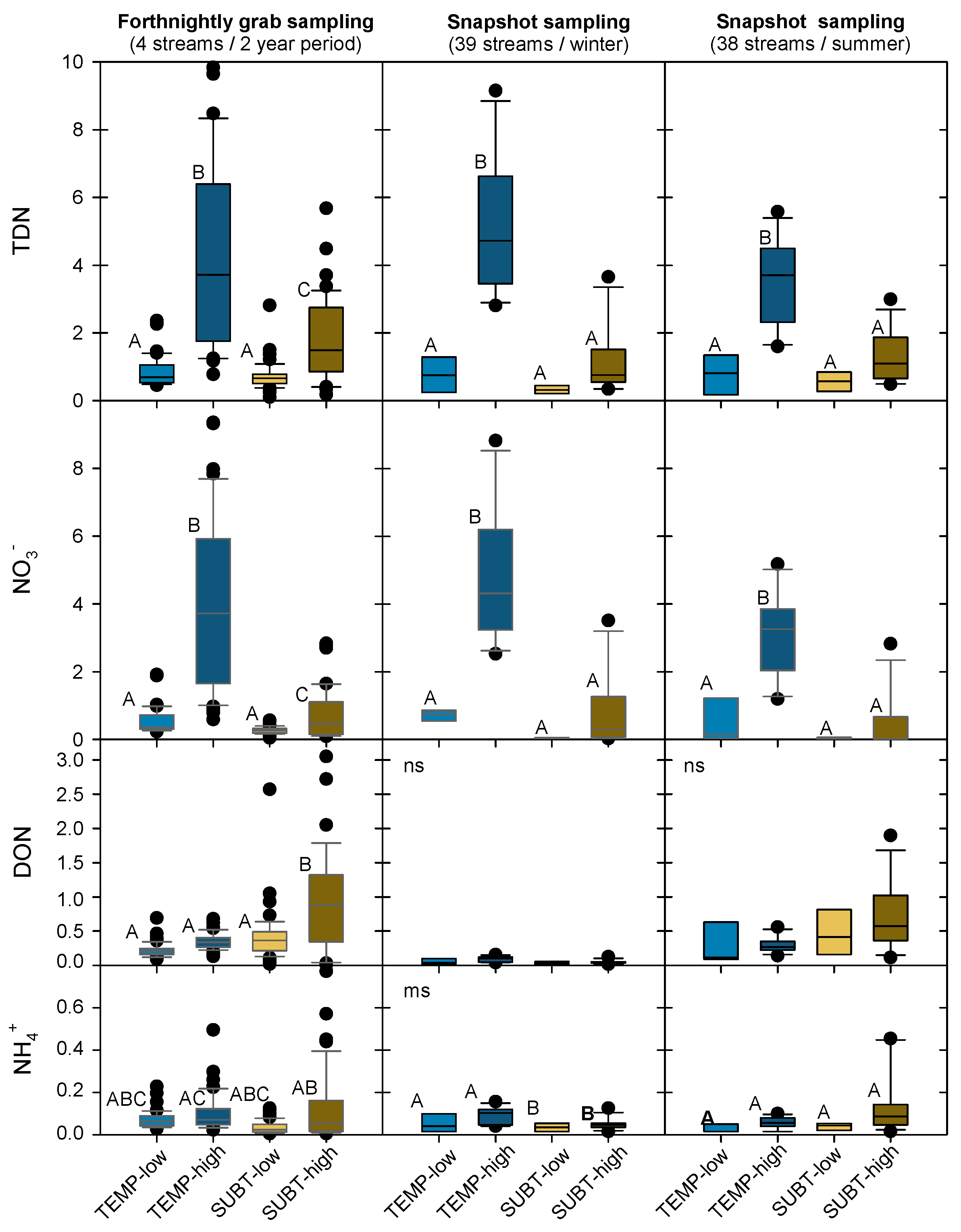
  • Fortnightly grab-sampling in benchmark streams: Sub-surface grab samples were taken from a well-mixed section with no macrophytes in the center of the stream channel during the daytime. This instantaneous sampling was used for the analysis of conservative and non-conservative N fractions (i.e., TN, TDN, NO3, DON, and NH4+).
  • Automatic pooled sampling in benchmark streams: High-frequency monitoring using automated equipment was conducted during the same two-year period. Glacier refrigerated automatic samplers (ISCO-Teledyne) collected an equal water volume every four hours from the same sampling point, and the pooled samples were collected fortnightly. The final nutrient concentration in the only sampler carboy thus represented a time-proportional average for the fortnightly sampling period. As this sampling involved refrigerated storage of pooled samples for up to two weeks, the emphasis was placed on the analysis of TN.
  • Snapshot grab-sampling in the series of streams was made once in winter and once in summer. Sub-surface grab samples were taken in a well-mixed section with no macrophytes from the center of the stream channels during the daytime. This instantaneous sampling was used for the analysis of different N fractions, with emphasis on dissolved compounds (i.e., TDN, NO3, DON, and NH4+).

2.3. Laboratory Measurements

All pooled water samples from the high frequency monitored streams were analyzed for total N (TN), total dissolved N (TDN), and nitrate (NO3). Analysis of fortnightly and snapshot samples included TN, TDN, NO3, NH4+, and DON (dissolved organic N). Different techniques were applied to guarantee accuracy, address the different concentration ranges, and assure the inter-comparability of results between countries.
Water samples for the determination of dissolved N fractions were filtered through 0.45-µm membrane filters pre-rinsed with ultrapure water (Milli-Q water). TN was converted to nitrate following the protocol of Valderrama [37] and analyzed as NO3. In Uruguay, the standard sodium salicylate method was used for NO3 determination [38,39]. For the Danish samples, the sum of both nitrate and nitrite was determined by flow analysis (CFA and FIA) and spectrometric detection ([40], Danish Standard 223). Additionally, the samples were analyzed by segmented flow analysis including an additional channel to measure NO2. As the NO2 concentration was always below the quantification limit of the technique (<0.01 mg N·L−1), it was not considered in the analysis; instead we assumed that (NO3) + (NO2) = (NO3).
The analysis of the Uruguayan samples used for total TDN determination followed the same approach as for the TN samples. The TDN concentrations of the Danish samples were measured using high-temperature catalytic oxidation (HTCO, multi N/C 3100, Jena Analytik, Jena, Germany) after acidifying the samples to pH 2–3 with HCl and sparging with synthetic air for 5 min. The samples were oxidized with a platinum catalyst at 700 °C in a synthetic air stream, and TDN was measured as NO gas with a chemiluminescence detector [41]. For the Danish water samples with high NO3 levels (from high-intensity farming), the HTCO method led to significant underestimation of TDN, likely because the HTCO method did not permit oxidization of all the N [42,43]. When oxidation was not possible, TDN was estimated as the addition of DIN + DON, DIN being in turn estimated as the addition of NO3 and NH4+ and DON being measured by size-exclusion chromatography [43,44]. DON samples taken in subtropical streams were acidified with hydrochloric acid and frozen, following Hudson, et al. [45], and sent for analysis at the Leibniz-Institute of Freshwater Ecology and Inland Fisheries laboratory in Berlin. Before measurements, the samples were brought to the same target pH level of 7.5 ± 0.5 by neutralization with sodium hydroxide. NH4+ was measured following the indophenol-blue method [46].

2.4. Data Analysis

Non-linear regressions between stage and discharge at each monitoring station (rating curves) were fitted. Rating curves were used to generate a discharge data series with a 10-min resolution using the software HYMER (www.orbicon.com). Base flow index (BFI) was estimated for the complete data set from daily hydrographs using the automatic routine proposed by Arnold et al. [47] to set the magnitude of the groundwater contribution to the streamflow.
Total N concentrations were determined from the fortnightly samples, while the high frequency automatized pooled data were used to estimate the annual TN transport, loss, and flow-weighted TN concentrations in the subset of the four benchmark streams (2-year period). The TN transport was calculated by multiplying the TN concentration obtained from the pooled samples by the accumulated discharge for the same fortnightly period and summing yearly [48]. The TN loss was calculated dividing the annual transport by the catchment area in hectares [49]. Missing data from the relatively short periods when the automatic samplers were not in operation (e.g., due to freezing in Denmark) were re-generated through linear interpolation of concentrations [50]. The flow-weighted concentration (FWC) was calculated as the annual TN transport divided by the annual runoff. Dissolved N fractions were analyzed from both the fortnightly grab samples in the four benchmark streams (2-year period) and the snapshot samples (nstreams = 39 winter, 38 summer; 1 sample per season).
The factorial design relative to climate/hydrology conditions and farming intensity was evaluated using two-way nested ANOVA with farming intensity nested within climate/hydrology, followed by a post hoc pairwise multiple comparison when appropriate [51]. Variability in the high frequency-automatized pooled and fortnightly samples represents the temporal variation within each intensively sampled stream, while variability in the snapshot sampling expresses spatial variation among comparable systems. The relationship between TN concentrations from the fortnightly instantaneous grab samples, discharge, and water temperature were analyzed by Spearman rank-order correlations.

3. Results

3.1. Climate and Hydrology

The climatic characteristics in the study period (2010 to early 2012) can be considered typical for both Denmark and Uruguay (Table 2; [30]). The annual average air temperature did not exhibit any anomaly [52,53] and corresponded to the mean for the corresponding region recorded by national meteorological services based on recent historical information [54,55]. Mean air temperature was 8.8 °C and ranged between −7.0 and 20.4 °C in the temperate sites and was ca. 17.5 °C, ranging between 3.7 to 32.2 °C, in the subtropical sites. No dry or wet seasons occurred in either country, but marked differences in frequency and intensity of rainfall were detected. Total annual precipitation was lower in the Danish catchments than in the Uruguayan catchments (Table 2), while rain events were less intense but more frequent in the Danish than in the Uruguayan catchments [30,31]. Thus, hydrologically, the Danish streams are more stable than the Uruguayan catchments, the latter being described as “flashy” in previous publications (Richards-Baker Flashinnes Index < 0.3 for Danish streams and > 0.9 for comparable Uruguayan streams; [30]). The Danish stable streams have much higher contribution of groundwater to water flow (higher base flow index, Table 2).

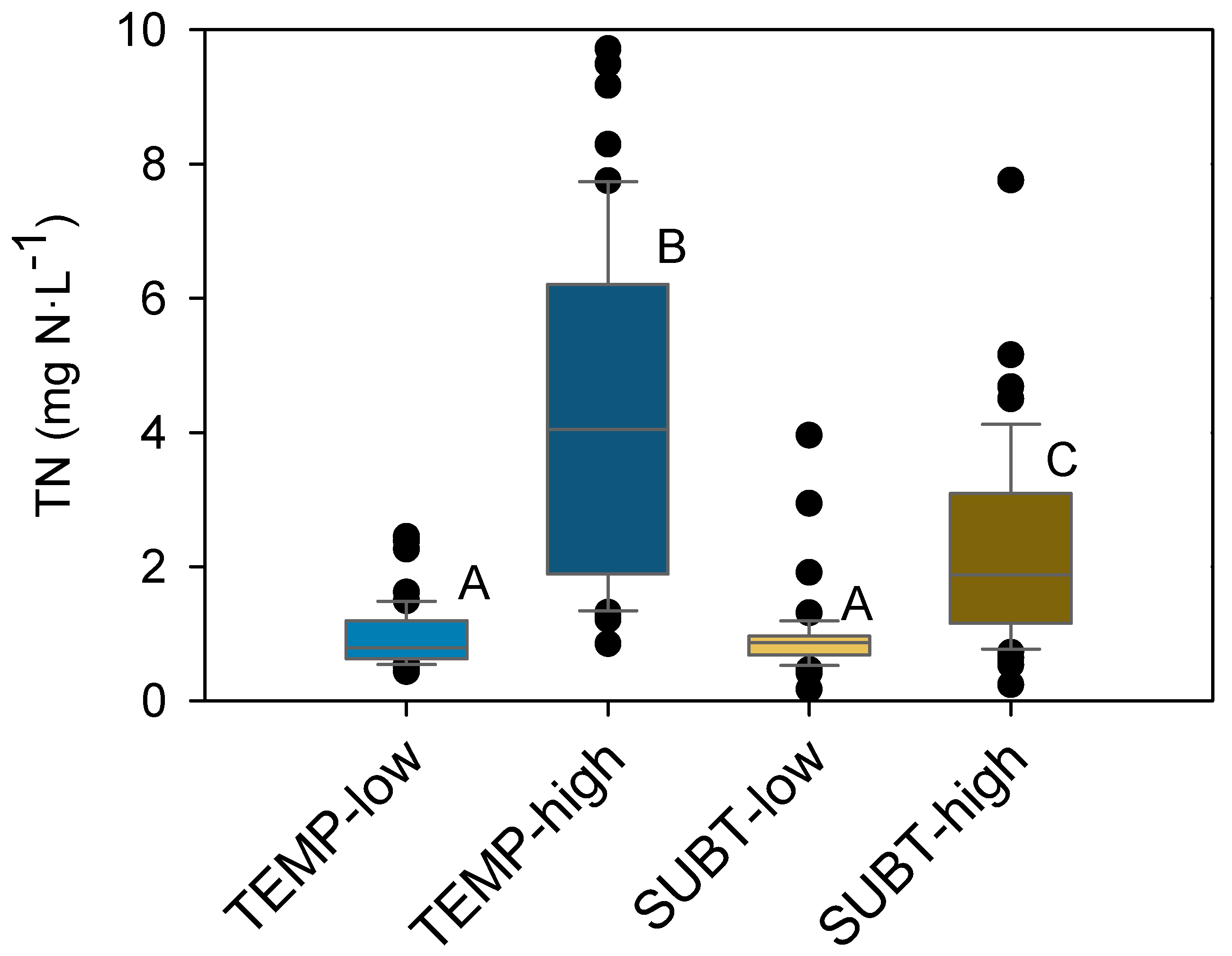
3.2. Total Nitrogen Concentrations and Losses in Benchmark Streams

The farming intensity was, as expected, a strong determinant factor of stream TN concentrations, while climate/hydrology had no significant effects on the TN concentrations in the benchmark streams (Figure 2). This was expressed by low and not statistically different TN concentrations in the low-farming intensity streams (varying around 1.0 mg N·L−1) and significantly higher average annual TN concentrations in high-intensity farming streams (2.2 ± 1.4 mg N·L−1 and 4.3 ± 2.5 mg N·L−1 for the subtropical and temperate high-intensity farming streams, respectively; mean ± SD; Figure 2). Total N loss and flow-weighted concentrations of TN (TN-FWC) obtained through high frequency-automatized pooled sampling were also higher in the highest intensity farming streams for both climatic/hydrological conditions (annual estimations for two years, no statistical testing possible; Table 3).
Without trends associated with farming intensity, the total N lost from subtropical catchments was between 2% and 4% of the total annual inputs as fertilizers and manure (Table 1 and Table 3). For the case of temperate catchments, the total N lost by the stream was 9% for high-intensity farming streams and between 10% and 14% (year 1 and 2 of monitoring) in low-intensity farming streams (Table 1 and Table 3).

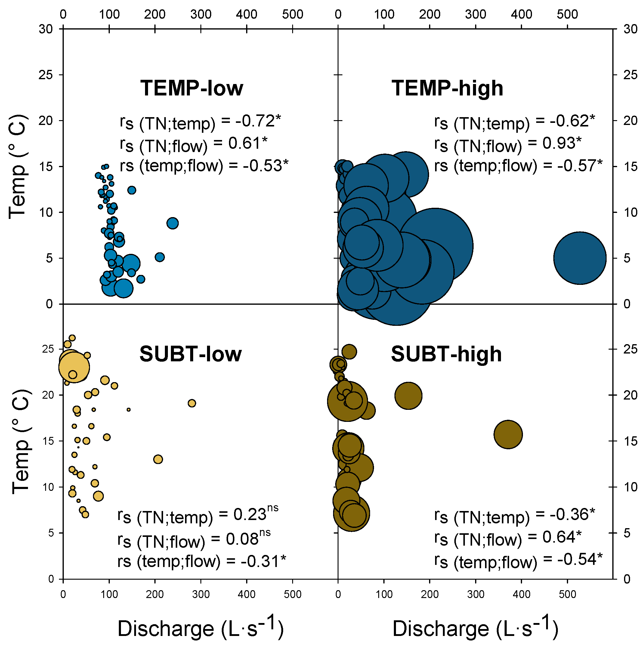
3.3. Influence of Temperature and Discharge on Total Nitrogen Concentrations

Stream TN concentrations tended to decrease with increasing water temperature and decreasing discharge, as reflected in the set of four fortnightly sampled benchmark streams (Figure 3). In both climates, the relationship between TN concentrations and discharge showed a higher explained variance for high-intensity farming than for low-intensity farming (Figure 3). The TN concentration of subtropical low-intensity farming stream, however, did not exhibit statistical relationships with temperature and discharge (Figure 3).

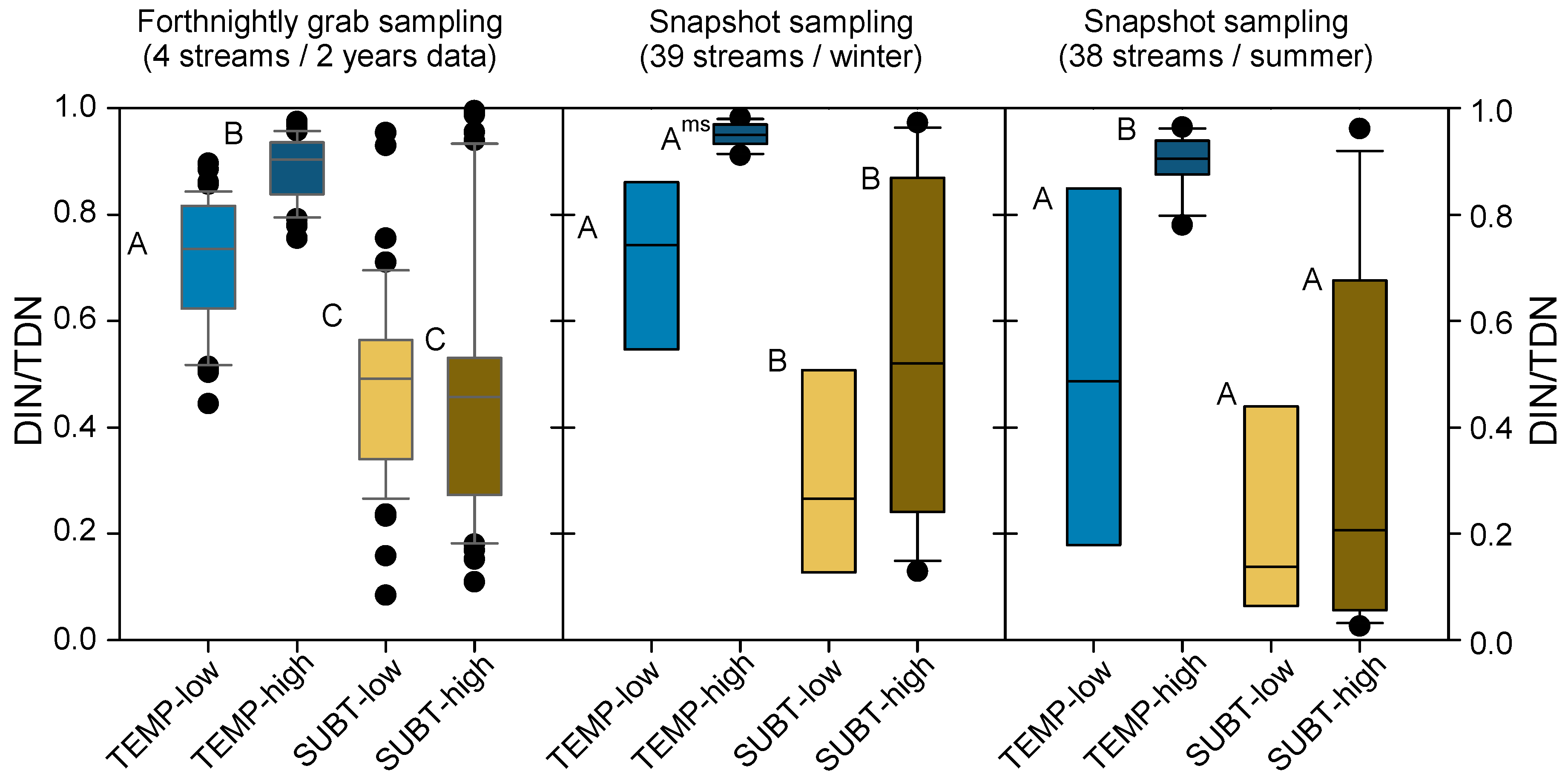
3.4. Influence of Climate/Hydrology and Farming Intensity on Nitrogen Species

Total dissolved N (TDN) constituted the main fraction of TN in all the studied streams (Figure 2 and Figure 4). It was also affected by farming intensity regardless of climate/hydrological conditions and monitoring method/sampling time (Table 4; Figure 4). These assertions are based on the comparable results obtained in all the sampled streams (n = 43), including both monitoring schemes: fortnightly grab sampling in benchmark streams and snapshot sampling (the analyses of this section include all these data sets; see Figure 4).
Relatively low (range of averages: 0.4 to 0.9 mg N·L−1), and not statistically different average TDN concentrations were found in all low-intensity farming streams, intermediate concentrations were found in the subtropical-high intensity farming streams (1.2 to 1.8 mg N·L−1), and the highest concentrations occurred in the temperate high-intensity farming streams (3.5 to 5.2 mg N·L−1; Table 4; Figure 4 upper panels). The pattern of intermediate TDN concentrations in the subtropical high-intensity farming streams was similar for the two sampling strategies, the only significant difference with low-intensity farming streams occurring for the fortnightly samples (Table 4; Figure 4).
Nitrate (NO3) concentrations resembled the above TN and TDN: low and not statistically different NO3 concentrations in the low-intensity farming streams, intermediate in the subtropical high-intensity farming streams, and the highest in the temperate high-intensity farming streams (complete data set; Table 4; Figure 4). Average annual NO3 concentrations ranged between values as low as 0.05 and 0.3 mg N·L−1 in the low-intensity farming streams in both climates (Figure 4). Average nitrate concentrations in the subtropical high-intensity farming streams ranged between 0.4 and 0.8 mg N·L−1. In contrast, in the temperate high-intensity farming streams, nitrate varied between 3.2 and 4.9 mg N·L−1 on average, depending on the sampling method and season (Figure 4).
We found no significant association between DON concentrations and climate/hydrological conditions or farming intensity, except for significantly higher levels of DON in the subtropical high-intensity farming streams (benchmark streams only, average = 0.9 mg N·L−1; Figure 4). All the other streams representing both climatic conditions had average levels below 0.7 mg N·L−1 (Table 4; Figure 4).
No significant relationships were found between ammonium (NH4+) concentrations and climate/hydrological conditions and farming intensity (fortnightly grab sampling in benchmark streams and snapshot sampling in summer; Table 4; Figure 4). Average NH4+ concentrations were always < 0.1 mg N·L−1, regardless of climate and farming intensity. In the wintry snapshot sampling, average NH4+ concentrations were significantly higher in the temperate (average 0.08 mg N·L−1) than in the subtropical streams (0.04 mg N·L−1; Table 4; Figure 4).
The DIN/TDN ratio was higher in the temperate (average ranging from 0.5 to almost 1) than in the subtropical streams (average ranging from 0.2 to 0.5) for the fortnightly and snapshot sampled streams (Table 4; Figure 5). The temperate high-intensity farming streams exhibited the highest DIN/TDN ratios (average between 0.89 and 0.95), which was linked to the strong predominance of NO3 (Figure 4 and Figure 5). In general, higher variability in the DIN/TDN ratio was observed in the subtropical streams (SD ranging from 0.2 to 0.3; Figure 5) than in the temperate streams.

4. Discussion

4.1. Influence of Farming Intensity

Our analysis of streams draining microcatchments under low-intensity farming conditions in contrasting climatic-hydrological settings revealed low and quite comparable TN, TDN, NO3, NH4+, and DON concentrations. In addition, NO3 concentrations in low-intensity farming streams at both climate/hydrological conditions exhibited levels that were considered as background concentrations in a recent and independent study conducted for streams draining relatively undisturbed catchments in Denmark and elsewhere [57]. No reference data for background concentrations in Uruguayan or subtropical streams have previously been reported in the scientific literature.
In contrast, the highest concentrations of NO3 were found in all sampled streams draining microcatchments impacted by high-intensity farming, irrespective of the monitoring method. Annual flow-weighted concentrations of TN never exceeded 1.2 mg N·L−1 in the two benchmark streams draining low intensity farmed catchments, but they were always higher than 2.0 mg N·L−1 in the two benchmark streams draining high intensity farmed catchments. The higher NO3 concentrations in the water (leading to higher concentrations of TDN and TN) can, therefore, be attributed to the impact of intensive farming in the catchments.
The TN, TDN, NO3, and TN-FWC concentrations in the streams draining high-intensity farming catchments were significantly higher in the temperate climate, with stable discharge conditions than in the subtropical climate with flashy discharge conditions.
The N input to the catchments as fertilizer and manure, was higher in subtropical than in temperate catchments, particularly by the higher contribution of manure derived from higher livestock loads. Contrarily, the N loss/N input fraction was higher in temperate catchments (9% to 14%), respect to subtropical ones (2% to 4%). Further, more detailed studies must be done to establish if assumptions made about N content of manure for Uruguay are correct, or if our results could be biased by it. Notwithstanding, these results are consistent with the much longer history of intensive farming in central and northern Europe than in South America, creating a potentially high N legacy in the groundwater feeding the streams [58,59,60]. Moreover, the widespread use of artificial drainage practices via tile drains in Danish productive catchments is a shortcut pathway for nitrate from the soils to surface waters; thus avoiding attenuation processes in groundwater [61,62,63,64]. Accordingly, the streams draining the temperate high intensity farmed catchments were characterized by higher NO3 concentrations and a larger contribution of groundwater to the total flow measured (higher base flow index, BFI) than in similar subtropical streams.
The concentrations of NH4+ and DON in streams did not show any clear relationship with the analyzed environmental factors. The proportional contribution of DON to TDN in the subtropical streams was, however, higher than in the temperate streams, which might be explained by the moderate to low levels of NO3 observed in the subtropical streams.
The global use of N fertilizers increases steadily [65], and the trend is forecasted to continue for the next decades despite more efficient management practices [66]. In the absence of a significant increase in N use efficiency (or the introduction of other retention or mitigation measures), the expected farming intensification in the future will result in an increase in N concentrations and losses in streams, which will further exacerbate eutrophication in surface freshwater bodies.

4.2. Influence of Climate

Benchmark streams showed statistically significant relationships between N concentrations and water temperature (negative) and discharge (positive). The former may be linked with high temperature-driven denitrification and higher N assimilation by aquatic macrophytes and periphyton in summer [65,66,67]. The latter, in contrast, may be explained by the N legacy in groundwaters in the intensively farmed catchments together with the annual N surplus and hence diffuse N contributions from agriculture in the catchments (leading to higher NO3 and TN concentrations in streams with increasing discharges). The lack of a significant relationship between N concentrations and temperature and discharge in the subtropical stream draining the low intensity farmed catchment was probably caused by the extremely low or lack of N surplus and N legacy, together with high denitrification and biological N uptake promoted by the higher temperatures.
Our results suggest that in a stationary scenario of farming intensity and management, warming alone might promote a reduction of TN concentrations in lowland low-order streams driven mainly by a reduction in NO3 concentrations. In contrast, the predicted increase in annual precipitation and the enhanced intensity of precipitation events in both countries [67,68,69] will probably increase the risk of diffuse N losses to streams, at least in intensively farmed catchments. Consequently, given these contradictory trends, it is uncertain what will be the resulting impact of climate change on N concentrations and losses in lowland streams in different climates and agricultural systems [70]. Several model scenario studies of climate change effects on N cycling in catchments have, however, suggested increases in exported N in the temperate climate regions [71,72]. The sense of the changes that the water tables suffer (e.g., height, residence time) probably will be one of the most influential factors regarding the N loss towards the streams. If the increase in flow regime variability, flashiness, and enhanced evapotranspiration results in a decrease in the contribution of groundwater [12], a lowering of the NO3 concentration and DIN/TDN ratio could be expected. Nevertheless, if the increasing precipitations get more infiltration, higher groundwater tables, and longer periods with tile drain flow, the effects could be the contrary.

5. Conclusions

The results from our three complementary monitoring approaches were broadly comparable and support that farming intensity is of key importance for determining N concentrations and losses in lowland streams, despite differences in soil and climatic-hydrological conditions between and within regions.
Overall, farming intensity determines the concentrations of TN, TDN, and NO3, flow-weighted TN, and TN exported to streams, but not those of ammonium (NH4+) and dissolved organic N (DON).
In the absence of a significant increase in farming N use efficiency (or the introduction of other palliative measures), the expected farming intensification will result in a stronger increase in NO3, TDN, and TN concentrations as well as rising flow-weighted N concentrations and N losses in temperate and subtropical streams, further exacerbating eutrophication.
In contrast to our expectations, a high dissolved inorganic N (DIN) to TDN ratio was associated with temperate climate and high base flow conditions but not with farming intensity.
The consequences of changes in climate for the streams in the studied countries are hard to predict as higher temperatures and higher precipitation had contrasting effects on TN concentrations in our study.

Author Contributions

Conceptualization, B.K., E.J., M.M., and G.G.; data curation, G.G. and D.G.; formal analysis, G.G.; funding acquisition, B.K., E.J., and M.M.; investigation, all authors; project administration, M.M.; supervision, B.K., E.J., and M.M.; visualization, G.G.; writing—original draft preparation, G.G.; writing—review and editing, D.G., M.M., E.J., F.T.-d.M., N.V., N.M., and B.K. All authors have read and agreed to the published version of the manuscript.

Funding

The study was funded by the Danish Council for Independent Research, a grant by ANII-FCE (2009-2749) Uruguay, and the National L’Oreal-UNESCO Award for Women in Science-Uruguay with support from DICyT granted to MM. GG, FTM, MM, IGB, and NM received support from the SNI (Agencia Nacional de Investigación e Inovación, ANII, Uruguay). GG was supported by a Ph.D. scholarship from PEDECIBA. E.J. and D.G. were further supported by MARS (Managing Aquatic ecosystems and water Resources under multiple Stress) funded under the 7th EU Framework Programme, Theme 6 (Environment including Climate Change), Contract No.: 603378 (http://www.mars-project.eu). DG was also supported by a grant from the Danish Centre for Environment and Energy.

Acknowledgments

We thank the technicians of AU in Silkeborg for their work in the field and lab. In Uruguay, we are grateful for the field assistance from Iván González-Bergonzoni, Natalie Corrales, Anahí López-Rodríguez, Clementina Calvo, Gonzalo Moreno, Alfonsina López, Carlos Iglesias, Juan Clemente, Mariana Vianna, and Juan Pablo Pacheco, and also to Verónica Ciganda, Diego Michelini and Carlos Perdomo for their generosity sharing agronomic information. We thank especially Daniella Agrati and family and the landowners (Mendiverri & Laturre) in Uruguay.

Conflicts of Interest

The authors declare no conflict of interest. The funders had no role in the design of the study; in the collection, analyses, or interpretation of data; in the writing of the manuscript, or in the decision to publish the results.

References

  1. Foley, J.A.; DeFries, R.; Asner, G.P.; Barford, C.; Bonan, G.; Carpenter, S.R.; Chapin, F.S.; Coe, M.T.; Daily, G.C.; Gibbs, H.K.; et al. Global consequences of land use. Science 2005, 309, 570–574. [Google Scholar] [CrossRef] [PubMed] [Green Version]
  2. Gordon, L.J.; Peterson, G.D.; Bennet, E.M. Agricultural modifications of hydrological flows create ecological surprises. Trends Ecol. Evol. 2008, 23, 211–219. [Google Scholar] [CrossRef] [PubMed]
  3. Erisman, J.W.; Sutton, M.A.; Galloway, J.; Klimont, Z.; Winiwarter, W. How a century of ammonia synthesis changed the world. Nat. Geosci. 2008, 1, 636–639. [Google Scholar] [CrossRef]
  4. Gruber, N.; Galloway, J.N. An Earth-system perspective of the global nitrogen cycle. Nature 2008, 451, 293–296. [Google Scholar] [CrossRef]
  5. Vitousek, P.M. Beyond global warming: Ecology and global change. Ecology 1994, 75, 1861–1876. [Google Scholar] [CrossRef]
  6. Carpenter, S.R.; Caraco, N.F.; Correll, D.L.; Howarth, R.W.; Sharpley, A.N.; Smith, V.H. Nonpoint pollution of surface waters with phosphorus and nitrogen. Ecol. Appl. 1998, 8, 559–568. [Google Scholar] [CrossRef]
  7. González-Sagrario, M.A.; Jeppesen, E.; Goma, J.; Søndergaard, M.; Jensen, J.; Lauridsen, T.L.; Lankildehus, F. Does high nitrogen loading prevent clear-water conditions in shallow lakes at moderately high phosphorus concentrations? Freshw. Biol. 2005, 50, 27–41. [Google Scholar] [CrossRef]
  8. James, C.; Fisher, J.; Russell, V.; Collings, S.; Moss, B. Nitrate availability and plant species richness: Implications for management of freshwater lakes. Freshw. Biol. 2005, 50, 49–63. [Google Scholar] [CrossRef]
  9. Steffen, W.; Richardson, K.; Rockström, J.; Cornell, S.E.; Fetzer, I.; Bennett, E.M.; Biggs, R.; Carpenter, S.R.; de Vries, W.; de Wit, C.A.; et al. Planetary boundaries: Guiding human development on a changing planet. Science 2015, 347, 1259855. [Google Scholar] [CrossRef] [Green Version]
  10. Bormann, F.H.; Likens, G.E. Nutrient cycling. Science 1967, 155, 424–428. [Google Scholar] [CrossRef]
  11. Boulêtreau, S.; Salvo, E.; Lyautey, E.; Mastrorillo, S.; Garabetian, F. Temperature dependence of denitrification in phototrophic river biofilms. Sci. Total Environ. 2012, 416, 323–328. [Google Scholar] [CrossRef] [PubMed]
  12. Deelstra, J.; Iital, A.; Povilaitis, A.; Kyllmar, K.; Greipsland, I.; Blicher-Mathiesen, G.; Jansons, V.; Koskiaho, J.; Lagzdins, A. Hydrological pathways and nitrogen runoff in agricultural dominated catchments in Nordic and Baltic countries. Agric. Ecosyst. Environ. 2014, 195, 211–219. [Google Scholar] [CrossRef]
  13. Exner-Kittridge, M.; Strauss, P.; Blöschl, G.; Eder, A.; Saracevic, E.; Zessner, M. The seasonal dynamics of the stream sources and input flow paths of water and nitrogen of an Austrian headwater agricultural catchment. Sci. Total Environ. 2016, 542 Pt A, 935–945. [Google Scholar] [CrossRef] [PubMed] [Green Version]
  14. Durand, P.; Breuer, L.; Johnes, P.J.; Billen, G.; Butturini, A.; Pinay, G.; van Grinsven, H.; Garnier, J.; Rivett, M.; Reay, D.S.; et al. Nitrogen processes in aquatic ecosystems. In The European Nitrogen Assessment—Sources, Effects and Policy Perspectives; Sutton, M.A., Howard, C.M., Erisman, J.W., Billen, G., Bleeker, A., Grennfelt, P., Eds.; Cambridge University Press: Cambridge, UK, 2011; p. 664. [Google Scholar]
  15. Huang, J.C.; Lee, T.Y.; Lin, T.C.; Hein, T.; Lee, L.C.; Shih, Y.T.; Kao, S.J.; Shiah, F.K.; Lin, N.H. Effects of different N sources on riverine DIN export and retention in a subtropical high-standing island, Taiwan. Biogeosciences 2016, 13, 1787–1800. [Google Scholar] [CrossRef] [Green Version]
  16. Sharpley, A.N.; Smith, S.J.; Naney, J.W. Environmental impact of agricultural nitrogen and phosphorus use. J. Agric. Food Chem. 1987, 35, 812–817. [Google Scholar] [CrossRef]
  17. Alexandratos, N.; Bruinsma, J. World Agriculture Towards 2030/2050: The 2012 Revision; FAO: Rome, Italy, 2012; Volume 12-03, p. 153. [Google Scholar]
  18. Lambin, E.F.; Geist, H.J.; Lepers, E. Dynamics of land-use and land-cover change in tropical regions. Annu. Rev. Environ. Res. 2003, 28, 205–241. [Google Scholar] [CrossRef] [Green Version]
  19. Potter, P.; Ramankutty, N.; Bennett, E.M.; Donner, S.D. Characterizing the spatial patterns of global fertilizer application and manure production. Earth Interact. 2010, 14, 1–22. [Google Scholar] [CrossRef]
  20. Potter, P.; Ramankutty, N.; Bennett, E.M.; Donner, S.D. Global Fertilizer and Manure, Version 1: Nitrogen Fertilizer Application; NASA Socioeconomic Data and Applications Center (SEDAC): Palisades, NY, USA, 2011. [Google Scholar]
  21. Allan, J.D.; Castillo, M.M. Stream Ecology: Structure and Function of Running Waters; Springer: Dordrecht, The Netherlands, 2007; p. 436. [Google Scholar]
  22. Dudgeon, D. Tropical Stream Ecology; Academic Press/Elsevier: London, UK, 2008; p. 324. [Google Scholar]
  23. Bustamante, M.M.C.; Martinelli, L.A.; Pérez, T.; Rasse, R.; Ometto, J.P.; Pacheco, F.S.; Lins, S.R.M.; Marquina, S. Nitrogen management challenges in major watersheds of South America. Environ. Res. Lett. 2015, 10, 065007. [Google Scholar] [CrossRef] [Green Version]
  24. Gücker, B.; Silva, R.C.S.; Graeber, D.; Monteiro, J.A.F.; Brookshire, E.N.J.; Chaves, R.C.; Boëchat, I.G. Dissolved nutrient exports from natural and human-impacted Neotropical catchments. Glob. Ecol. Biogeogr. 2016, 25, 378–390. [Google Scholar] [CrossRef]
  25. Follett, R. Chapter 2. Transformation and transport processes of nitrogen in agricultural systems. In Nitrogen in the Environment: Sources, Problems, and Management, 2nd ed.; Hatfield, J.L., Follett, R.F., Eds.; Academic Press/Elsevier: San Diego, CA, USA, 2008; pp. 19–50. [Google Scholar]
  26. Phalan, B.; Bertzky, M.; Butchart, S.H.M.; Donald, P.F.; Scharlemann, J.P.W.; Stattersfield, A.J.; Balmford, A. Crop expansion and conservation priorities in tropical countries. PLoS ONE 2013, 8, e51759. [Google Scholar] [CrossRef] [Green Version]
  27. Laurance, W.F.; Sayer, J.; Cassman, K.G. Agricultural expansion and its impacts on tropical nature. Trends Ecol. Evol. 2014, 29, 107–116. [Google Scholar] [CrossRef] [PubMed]
  28. Schindler, D.W. Replication versus realism: The need for ecosystem-scale experiments. Ecosystems 1998, 1, 323–334. [Google Scholar] [CrossRef]
  29. Peel, M.C.; Finlayson, B.L.; McMahon, T.A. Updated world map of the Köppen-Geiger climate classification. Hydrol. Earth Syst. Sci. 2007, 11, 1633–1644. [Google Scholar] [CrossRef] [Green Version]
  30. Goyenola, G.; Meerhoff, M.; Teixeira-de Mello, F.; González-Bergonzoni, I.; Graeber, D.; Fosalba, C.; Vidal, N.; Mazzeo, N.; Ovesen, N.B.; Jeppesen, E.; et al. Monitoring strategies of stream phosphorus under contrasting climate-driven flow regimes. Hydrol. Earth Syst. Sci. 2015, 19, 4099–4111. [Google Scholar] [CrossRef] [Green Version]
  31. Graeber, D.; Goyenola, G.; Meerhoff, M.; Zwirnmann, E.; Ovesen, N.B.; Glendell, M.; Gelbrecht, J.; Teixeira de Mello, F.; González-Bergonzoni, I.; Jeppesen, E.; et al. Interacting effects of climate and agriculture on fluvial DOM in temperate and subtropical catchments. Hydrol. Earth Syst. Sci. 2015, 19, 2377–2394. [Google Scholar] [CrossRef] [Green Version]
  32. Blicher-Mathiesen, G.; Rasmussen, A.; Grant, R.; Jensen, P.G.; Hansen, B.; Thorling, L. Landovervågningsoplande 2012. NOVANA; Aarhus Universitet, DCE—Nationalt Center for Miljø og Energi, 2013; p. 154, Videnskabelig Rapport fra DCE—Nationalt Center for Miljø og Energi nr. 174; Available online: http://dce152.au.dk/pub/SR74.pdf (accessed on 1 April 2020).
  33. Ciganda, V. Instituto Nacional de Investigación Agropecuaria, La Estanzuela; Personal Communication: Colonia, Uruguay, 2020. [Google Scholar]
  34. Brown, M.T.; Vivas, M.B. Landscape development intensity index. Environ. Monit. Assess. 2005, 101, 289–309. [Google Scholar] [CrossRef]
  35. Blüthgen, N.; Dormann, C.F.; Prati, D.; Klaus, V.H.; Kleinebecker, T.; Hölzel, N.; Alt, F.; Boch, S.; Gockel, S.; Hemp, A.; et al. A quantitative index of land-use intensity in grasslands: Integrating mowing, grazing and fertilization. Basic Appl. Ecol. 2012, 13, 207–220. [Google Scholar] [CrossRef]
  36. Allaby, M. Grasslands; Chelsea House: New York, NY, USA, 2006; p. 270. [Google Scholar]
  37. Valderrama, J.C. The simultaneous analysis of total nitrogen and total phosphorus in natural waters. Mar. Chem. 1981, 10, 109–122. [Google Scholar] [CrossRef]
  38. Müller, R.; Weidemann, O. Die bestimmung des Nitrat-ions in wasser. Wasser 1955, 22, 247. [Google Scholar]
  39. Monteiro, M.I.C.; Ferreira, F.N.; de Oliveira, N.M.M.; Avila, A.K. Simplified version of the sodium salicylate method for analysis of nitrate in drinking waters. Anal. Chim. Acta 2003, 477, 125–129. [Google Scholar] [CrossRef]
  40. ISO13395. Water Quality—Determination of Nitrite Nitrogen and Nitrate Nitrogen and the Sum of Both by Flow Analysis (CFA and FIA) and Spectrometric Detection. Available online: http://www.iso.org/iso/catalogue_detail.htm?csnumber=21870 (accessed on 26 April 2016).
  41. Zwirnmann, E.; Krüger, A.; Gelbrecht, J. Analytik im Zentralen Chemielabor des IGB, Berichte des IGB, Heft 9; Institut Für Gewa¨Ssero¨Kologie und Binnenfischerei: Berlin, Germany, 1999. [Google Scholar]
  42. Lee, W.; Westerhoff, P. Dissolved organic nitrogen measurement using dialysis pretreatment. Environ. Sci. Technol. 2005, 39, 879–884. [Google Scholar] [CrossRef] [PubMed]
  43. Graeber, D.; Gelbrecht, J.; Kronvang, B.; Gücker, B.; Pusch, M.T.; Zwirnmann, E. Technical Note: Comparison between a direct and the standard, indirect method for dissolved organic nitrogen determination in freshwater environments with high dissolved inorganic nitrogen concentrations. Biogeosciences 2012, 9, 4873–4884. [Google Scholar] [CrossRef] [Green Version]
  44. Huber, S.; Balz, A.; Abert, M.; Pronk, W. Characterisation of aquatic humic and non-humic matter with size-exclusion chromatography—Organic carbon detection—Organic nitrogen detection (LC-OCD-OND). Water Res. 2011, 45, 879–885. [Google Scholar] [CrossRef] [PubMed]
  45. Hudson, N.; Baker, A.; Reynolds, D.; Carliell-Marquet, C.; Ward, D. Changes in freshwater organic matter fluorescence intensity with freezing/ thawing and dehydration/rehydration. J. Geophys. Res. Biogeosci. 2009, 114, G00F08. [Google Scholar] [CrossRef] [Green Version]
  46. Koroleff, F. Direct Determination of Ammonia in Natural Water as Indophenol-Blue; ICES: Copenhagen, Denmark, 1970; pp. 19–22. [Google Scholar]
  47. Arnold, J.G.; Allen, P.M.; Muttiah, R.; Bernhardt, G. Automated base flow separation and recession analysis techniques. Ground Water 1995, 33, 1010–1018. [Google Scholar] [CrossRef]
  48. Kronvang, B.; Bruhn, A.J. Choice of sampling strategy and estimation method for calculating nitrogen and phosphorus transport in small lowland streams. Hydrol. Process. 1996, 10, 1483–1501. [Google Scholar] [CrossRef]
  49. Smith, S.V.; Swaney, D.P.; Buddemeier, R.W.; Scarsbrook, M.R.; Weatherhead, M.A.; Humborg, C.; Eriksson, H.; Hannerz, F. River nutrient loads and catchment size. Biogeochemistry 2005, 75, 83–107. [Google Scholar] [CrossRef]
  50. Jones, A.S.; Horsburgh, J.S.; Mesner, N.O.; Ryel, R.J.; Stevens, D.K. Influence of sampling frequency on estimation of annual total phosphorus and total suspended solids loads. J. Am. Water Resour. Assoc. 2012, 48, 1258–1275. [Google Scholar] [CrossRef]
  51. Bonferroni, C.E. Teoria statistica delle classi e calcolo delle probabilità. Pubbl. Ist. Super. Sci. Econ. Commer. Firenze 1936, 8, 3–62. [Google Scholar]
  52. Hansen, J.; Ruedy, R.; Sato, M.; Lo, K. Global surface temperature change. Rev. Geophys. 2010, 48, RG4004. [Google Scholar] [CrossRef] [Green Version]
  53. GISTEMP Team. GISS Surface Temperature Analysis (GISTEMP). Available online: http://data.giss.nasa.gov/gistemp/ (accessed on 16 May 2016).
  54. DMI. Decadal Mean Weather. Available online: http://www.dmi.dk/en/vejr/arkiver/decadal-mean-weather/ (accessed on 26 April 2016).
  55. INUMET. Cilimatological Statistics. Available online: http://www.meteorologia.com.uy/ServCli/caracteristicasClimaticas (accessed on 26 April 2016).
  56. DMI. Denmark’s Future Climate. Available online: https://www.dmi.dk/en/klima/fremtidens-klima/danmark-og-groenland/ (accessed on 4 November 2016).
  57. Kronvang, B.; Windolf, J.; Larsen, S.E.; Bøgestrand, J. Background concentrations and loadings of nitrogen in Danish surface waters. Acta Agric. Scand. B Soil Plant 2015, 65, 155–163. [Google Scholar] [CrossRef]
  58. Hansen, B.; Dalgaard, T.; Thorling, L.; Sørensen, B.; Erlandsen, M. Regional analysis of groundwater nitrate concentrations and trends in Denmark in regard to agricultural influence. Biogeosciences 2012, 9, 3277–3286. [Google Scholar] [CrossRef] [Green Version]
  59. McLauchlan, K. The nature and longevity of agricultural impacts on soil carbon and nutrients: A review. Ecosystems 2006, 9, 1364–1382. [Google Scholar] [CrossRef]
  60. Tesoriero, A.J.; Duff, J.H.; Saad, D.A.; Spahr, N.E.; Wolock, D.M. Vulnerability of streams to legacy nitrate sources. Environ. Sci. Technol. 2013, 47, 3623–3629. [Google Scholar] [CrossRef]
  61. Grant, R.; Laubel, A.; Kronvang, B.; Andersen, H.E.; Svendsen, L.M.; Fuglsang, A. Loss of dissolved and particulate phosphorus from arable catchments by subsurface drainage. Water Res. 1996, 30, 2633–2642. [Google Scholar] [CrossRef]
  62. Andersen, H.E.; Windolf, J.; Kronvang, B. Leaching of dissolved phosphorus from tile-drained agricultural areas. Water Sci. Technol. 2016, 73, 2953–2958. [Google Scholar] [CrossRef]
  63. Schoumans, O.F.; Chardon, W.J.; Bechmann, M.E.; Gascuel-Odoux, C.; Hofman, G.; Kronvang, B.; Rubæk, G.H.; Ulén, B.; Dorioz, J.M. Mitigation options to reduce phosphorus losses from the agricultural sector and improve surface water quality: A review. Sci. Total Environ. 2014, 468–469, 1255–1266. [Google Scholar] [CrossRef]
  64. Windolf, J.; Thodsen, H.; Troldborg, L.; Larsen, S.E.; Bøgestrand, J.; Ovesen, N.B.; Kronvang, B. A distributed modelling system for simulation of monthly runoff and nitrogen sources, loads and sinks for ungauged catchments in Denmark. J. Environ. Monit. 2011, 13, 2645–2658. [Google Scholar] [CrossRef]
  65. FAO. World Fertilizer Trends and Outlook to 2018; FAO: Rome, Italy, 2015; p. 53. [Google Scholar]
  66. Tilman, D.; Balzer, C.; Hill, J.; Befort, B.L. Global food demand and the sustainable intensification of agriculture. Proc. Natl. Acad. Sci. USA 2011, 108, 20260–20264. [Google Scholar] [CrossRef] [Green Version]
  67. CDKN. The IPCC’s Fifth Assessment Report What’s in it for Latin America? Executive Summary. Available online: https://cdkn.org/wp-content/uploads/2014/11/IPCC-AR5-Whats-in-it-for-Latin-America.pdf (accessed on 1 April 2020).
  68. Madsen, H.; Arnbjerg-Nielsen, K.; Steen-Mikkelsen, P. Update of regional intensity–duration–frequency curves in Denmark: Tendency towards increased storm intensities. Atmos. Res. 2009, 92, 343–349. [Google Scholar] [CrossRef]
  69. Marengo, J.; Rusticucci, M.; Penalba, O.; Renom, M.; Laborbe, R. An intercomparison of observed and simulated extreme rainfall and temperature events during the last half of the twentieth century: Part 2: Historical trends. Clim. Chang. 2010, 98, 509–529. [Google Scholar] [CrossRef] [Green Version]
  70. Olesen, J.E.; Carter, T.R.; Díaz-Ambrona, C.H.; Fronzek, S.; Heidmann, T.; Hickler, T.; Holt, T.; Minguez, M.I.; Morales, P.; Palutikof, J.P.; et al. Uncertainties in projected impacts of climate change on European agriculture and terrestrial ecosystems based on scenarios from regional climate models. Clim. Chang. 2007, 81, 123–143. [Google Scholar] [CrossRef]
  71. Andersen, H.E.; Kronvang, B.; Larsen, S.E.; Hoffmann, C.C.; Jensen, T.S.; Rasmussen, E.K. Climate-change impacts on hydrology and nutrients in a Danish lowland river basin. Sci. Total Environ. 2006, 365, 223–237. [Google Scholar] [CrossRef] [PubMed]
  72. Jeppesen, E.; Kronvang, B.; Olesen, J.; Audet, J.; Søndergaard, M.; Hoffmann, C.; Andersen, H.; Lauridsen, T.; Liboriussen, L.; Larsen, S.; et al. Climate change effects on nitrogen loading from cultivated catchments in Europe: Implications for nitrogen retention, ecological state of lakes and adaptation. Hydrobiologia 2011, 663, 1–21. [Google Scholar] [CrossRef]
Figure 1. The geographic location of sampled streams. Left: subtropical/Uruguayan streams. Right: temperate/Danish streams. Circles: Snapshot grab-sampling. Stars: Benchmark streams. Green: high-farming intensity; brown: low-farming intensity. LAT/LONG of benchmark streams: TEMP Low: 56.2837/9.8975; TEMP High: 56.2254/9.8117; SUBT Low: −33.8256/−56.2821; SUBT Low: −33.9036/−56.0064. All the catchments fall within polygons limited by the following coordinates: Denmark 55.09 to 56.64 N; 8.38 to 12.44 E, Uruguay −31.79 to −34.18; −54.41 to −58.31 (decimal degrees; WGS84).
Water 12 01021 g001
Figure 2. Variability in total nitrogen (TN) concentrations for each of the four fortnightly grabs sampled benchmark streams. Data correspond to a 2-year period. ANOVA results: F TEMP vs. SUBT (1,190) = 23.73, Farming intensity conditions nested in climate/hydrology (2,190) = 70.44, F Interaction (1,190) = 378.9. P < 0.001 for all cases. A, B, and C describe statistically similar groups according to Bonferroni post hoc tests. The upper and lower boundaries of the box mark the 25th and 75th percentile, whiskers above and below the box indicate the 90th and 10th percentiles and the line within the box marks the median. Black dots display outliers. Abbreviations: TEMP: temperate streams; SUBT: subtropical streams; low and high: low and high-farming intensity in the catchments.
Water 12 01021 g002
Figure 3. Total nitrogen concentrations vs. water temperature and discharge in the subset of the four benchmark streams under high-frequency monitoring. Bubble size represents the concentration of TN from fortnightly grab sampling (two-year data). The graphs show the main environmental gradients for each stream. Spearman rank-order correlations (rs) are marked with * when significant (0.01 ≤ p ≤ 0.05). ns: non-significant. Abbreviations: TEMP: temperate streams; SUBT: subtropical streams; low and high: low and high-farming intensity in the catchments.
Water 12 01021 g003
Figure 4. The concentration of dissolved nitrogen fractions in fortnightly grab sampling in benchmark streams and snapshot samples. Significance level P < 0.05. A, B, and C describe statistical groups according to post hoc Bonferroni tests. We indicate non-significant results as ns (p > 0.1), and marginally significant as ms (0.05 < P < 0.1). Abbreviations: TEMP: temperate streams; SUBT: subtropical streams; low- and high-FI: low and high-farming intensity. Vertical axes are concentrations expressed in mg N·L−1. The upper and lower boundaries of the box mark the 25th and 75th percentile, whiskers above and below the box indicate the 90th and 10th percentiles and the line within the box marks the median. Black dots display outliers. Note that the scale varies among fractions.
Water 12 01021 g004
Figure 5. DIN/TDN ratio for the fortnightly grab sampling in benchmark streams and snapshot samples. Significance level P < 0.05. A, B, and C describe statistical groups according to post hoc Bonferroni tests. We indicate marginally significant as ms (0.05 < P < 0.1). The upper and lower boundaries of the box mark the 25th and 75th percentile, whiskers above and below the box indicate the 90th and 10th percentiles and the line within the box marks the median. Black dots display outliers. Note that the scale varies among fractions. Abbreviations: TEMP: temperate streams; SUBT: subtropical streams; low and high: low and high-farming intensity.
Water 12 01021 g005
Table 1. Characteristics of the soil and land-use of all the studied stream catchments according to the sampling method used. Benchmark streams were sampled fortnightly using grab and automatized pooled sampling.
Climate & Farming IntensityBenchmark StreamsSnapshot Grab-Sampling
TEMP LowGranslev stream
Haplic Luvisols # O.M. = 5%
F.A.= 29%; mean L.U. = 0.25 ha−1
N fertilizer = 45 kg N·ha−1·year−1
(45 % fertilizers; 55% manure)
Mainly Luvisols and Podsols; Arenosols #
O.M. < 5%. Range F.A. = 0%–26%
TEMP HighGelbæk stream
Gleyic Luvisols # O.M. < 5%
F.A.= 92%; mean L.U. = 0.79 ha−1
N fertilizer = 143 kg N·ha−1·year−1
(45 % fertilizers; 55% manure)
Mainly Luvisols and Podsols, some Albeluvisols Arenosols and Cambisols #
O.M. < 5%. Range F.A. = 74%–93%
SUBT LowChal-Chal stream
Luvic Phaeozem and
Eutric Vertisols * O.M. = 5.2%
F.A.= 30%; mean L.U. = 0.62 ha−1
N fertilizer = 76 kg N·ha−1·year−1
(18% fertilizers; 82% manure)
Phaeozem and Vertisols *
O.M. = 5% ± 1.5
Range F.A. = 0%–25%
SUBT HighPintado Stream
Eutric Regosols * O.M. = 4% to 5%
F.A.= 90%; mean L.U. = 2.00 ha−1
N fertilizer = 242 kg N·ha−1·year−1
(17% fertilizers; 83% manure)
Mainly Phaeozem *
O.M. = 5% ± 1.5
Range F.A. = 75%–100%
Total nnstreams = 4nstreams = 39 (w), 38 (s)
Samplinggrab and pooled sampling
2 years
1 sample in (w) and 1 in (s)
Abbreviations: TEMP: temperate streams; SUBT: subtropical streams; Low and High: low and high-farming intensity; O.M.: organic content of soils (%); F.A.: percentage of the Farming area; mean L.U.: mean livestock units by ha; N fertilizer: total N inputs by year, discriminated in contributions of fertilizers and manure. (w): winter; (s): summer. Source: (#) World Reference Soil Database classification, European Commission and European Soil Bureau Network (2004); (*) SOTERLAC database, ISRIC Foundation (www.isric.org).
Table 2. Main climatic and hydrological characteristics of the four benchmark catchments monitored at high frequency (nstreams = 4, 2-year period), showing annual accumulated rainfall in mm for each study year (sources: a [56], b [55]). Abbreviations: TEMP: temperate streams; SUBT: subtropical streams; Low and High: low and high-farming intensity.
CharacteristicTEMP
Low
TEMP
High
SUBT
Low
SUBT
High
Accumulated rainfall
of each study year (mm·y−1)
756–770766–7781010–10301196–1405
Mean regional
accumulated rainfall (mm·y−1)
765 a1100–1200 b
Base Flow Index (BFI)0.880.640.390.29
Table 3. Total nitrogen losses by hectare (kg N·ha−1·year−1) and flow-weighted concentrations (FWC; mg N·L−1) estimated annually using high frequency automatized pooled sampling of the four benchmark streams (water samples taken every 4 h and accumulated fortnightly). Abbreviations: TEMP: temperate streams; SUBT: subtropical streams; low and high: low and high-farming intensity in the catchments.
RegionYearLow-Farming IntensityHigh-Farming Intensity
TN LossFWC TNTN LossFWC TN
SUBT11.390.824.671.99
SUBT22.120.729.172.13
TEMP16.111.213.166.28
TEMP24.680.9812.656.23
Table 4. Summary of 2-way nested ANOVA tests for the concentration of N forms, indicating the origin (sampling method) of the data. Above: Main effects of climate/hydrology conditions (two levels). Below: Main effects of farming intensity (two levels: low- and high-intensity farming) nested within climate/hydrology conditions and interaction between factors. F values and the respective degrees of freedom are indicated. Significance level: P > 0.1 ns, 0.05 < P < 0.1 ms, P < 0.05 *, P < 0.01 **, P < 0.001 ***. Results of post hoc pairwise multiple comparisons are shown in Figure 3, Figure 4 and Figure 5. Abbreviations: TEMP: temperate streams; SUBT: subtropical streams; low and high: low- and high-farming intensity in the catchments.
N FormBenchmark StreamsSnapshot Sampling
Fortnightly SamplingWinterSummer
Comparison between Climate/Hydrology Conditions (TEMP vs. SUBT)
TDNF(1, 181) = 38.16 ***F(1, 35) = 29.97 ***F(1, 34) = 19.60 ***
NO3F(1, 186) = 78.25 ***F(1, 35) = 29.99 ***F(1, 34) = 30.58 ***
DONF(1, 181) = 27.27 ***F(1, 35) = 1.44, p = 0.24 nsF(1, 34) = 4.90 *
NH4+F(1, 186) = 0.19, p = 0.66 nsF(1 35) = 7.72 **F(1, 34) = 2.31, p = 0.14 ns
DIN/TDNF(1, 181) = 179.67 ***F(1, 35) = 30.06 ***F(1, 34) = 23.67 ***
Comparison between Farming Intensity Conditions (Low & High)
Nested in Climate/Hydrology
TDNF(2, 181) = 71.85 ***F(2, 35) = 30.30 ***F(2, 34) = 20.78 ***
NO3F(2, 186) = 80.12 ***F(2, 35) = 28.48 ***F(2, 34) = 20.49 ***
DONF(2, 181) = 24.42 ***F(2, 35) = 0.232, p = 0.79 nsF(2, 34) = 1.19, p = 0.31 ns
NH4+F(2, 186) = 10.05 ***F(2, 35) = 2.75, p = 0.08 msF(2, 34) = 3.09, p = 0.08 ms
DIN/TDNF(2, 181) = 14.67 ***F(2, 35) = 6.26 **F(2, 34) = 5.50**
Interaction between Farming Intensity and Climate/Hydrology
TDNF(1, 181) = 307.1 ***F(1, 35) = 85.0 ***F(1, 34) = 116.4 ***
NO3-F(1, 186) = 193.6 ***F(1, 35) = 57.5 ***F(1, 34) = 52.33 ***
DONF(1, 181) = 255.1 ***F(1 35) = 103.0 ***F(1, 34) = 59.9 ***
NH4+F(1, 186) = 140.3 ***F(1, 35) = 106.0 ***F(1, 34) = 21.6 ***
DIN/TDNF(1, 181) = 2744.1 ***F(1, 35) = 299.3 ***F(1, 34) = 132.9***

