Investigating Atrazine Concentrations in the Zwischenscholle Aquifer Using MODFLOW with the HYDRUS-1D Package and MT3DMS

Abstract

Simulation models that describe the flow and transport processes of pesticides in soil and groundwater are important tools to analyze how surface pesticide applications influence groundwater quality. The aim of this study is to investigate whether the slow decline and the stable spatial pattern of atrazine concentrations after its ban, which were observed in a long-term monitoring study of pesticide concentrations in the Zwischenscholle aquifer (Germany), could be explained by such model simulations. Model simulations were carried out using MODFLOW model coupled with the HYDRUS-1D package and MT3DMS. The results indicate that the spatial variability in the atrazine application rate and the volume of water entering and leaving the aquifer through lateral boundaries produced variations in the spatial distribution of atrazine in the aquifer. The simulated and observed water table levels and the average annual atrazine concentrations were found to be comparable. The long-term analysis of the simulated impact of atrazine applications in the study area shows that atrazine persisted in groundwater even 20 years after its ban at an average atrazine concentration of 0.035 µg/L. These results corroborate the findings of the previous monitoring studies.

1. Introduction

Pesticides are widely used all over the world to protect crops in agricultural fields. Uncontrolled and improper pesticide applications have led to their presence in the environment exceeding permissible limits [1,2,3,4]. It has been observed that groundwater is most affected by pesticide applications in agricultural fields [5,6,7,8,9]. The pesticide contamination of groundwater is generally assessed through pesticide monitoring programs (e.g., [10,11,12]). Once the information about pesticide concentrations in the groundwater is obtained, it is crucial to analyze the spatiotemporal relations between surface applications of pesticides and their groundwater concentrations. Such an analysis is important for several reasons: (a) to assess the role of non-point versus point scale sources of contamination, (b) to interpret observations of monitoring studies, (c) to identify vulnerable locations in the aquifer, and (d) to evaluate the effectiveness of various regulatory measures for protecting groundwater quality. The approaches that have been used for such assessments can be classified into (a) geostatistical approaches [13], and the use of (b) spatially distributed one-dimensional soil models [14], (c) groundwater models [15], and (d) coupled soil and groundwater models [16,17]. The latter type of modeling approaches can be used to assess the impact of various processes including groundwater flow and solute transport, dilution, and decay, as well as the impact of the spatial distribution of pesticide loadings to groundwater on the spatiotemporal patterns of pesticide concentrations in the groundwater [18,19]. In this study, we investigate whether the slow decline and stable spatial patterns of atrazine concentrations after its ban, that were observed in a long-term monitoring study of pesticide concentrations in the Zwischenscholle aquifer in Germany [20,21], could be explained by such model simulations.

Atrazine was one of the most widely applied pesticides for weed control worldwide [20,21,22,23,24]. There are many cases of atrazine contamination of the soil and groundwater reported in different parts of the world [25,26,27,28]. In Germany, atrazine was applied mainly in agricultural fields for maize cultivation. This pesticide was banned in March 1991, since concentrations in groundwater and drinking water were found to be exceeding the permissible limits. In Europe, according to the European Council Directive 98/83/EC “The quality of water intended for human consumption” (1998) [29], the threshold limit of pesticide concentrations is 0.1 μg/L for a single compound and 0.5 μg/L for the sum of all pesticides. Despite its ban, atrazine and its metabolite deethylatrazine were observed in German aquifers several years after its ban [24]. The Zwischenscholle aquifer in Germany is one of many aquifers in the world contaminated with atrazine [22,23]. Due to a shallow groundwater level and intensive agricultural land use in the Zwischenscholle aquifer, the vulnerability of this aquifer to pesticide contamination was found to be very high [24,30,31].

Vonberg et al. [20,21] conducted a detailed investigation of atrazine concentrations in the soil and groundwater of the Zwischenscholle aquifer. In their study, the analysis of the observations from a monitoring campaign of atrazine concentrations from 1991 to 2011 showed that the groundwater concentration of atrazine is still close to the threshold limit (0.1 μg/L even 20 years after its ban in 1991. The study demonstrated a considerable variation of atrazine concentrations in space and also concluded that the spatial pattern of the concentration distribution was relatively stable during the monitoring period.

Centered on the concluding remarks made by Vonberg et al. [20,21], the main objective of the current study was to investigate the atrazine contamination in the Zwischenscholle aquifer by analyzing the persistent nature of the atrazine concentration and its spatiotemporal pattern using a simulation model. There exist various approaches and methods for analyzing the aquifer contamination ranging from simple analytical to complex numerical methods. Analytical methods facilitate a basic and rapid preliminary analysis of the groundwater contamination but are generally associated with a number of simplifying assumptions regarding the groundwater system. They are limited to simple aquifer geometries and homogeneous aquifer properties [32,33]. Some of the methods of groundwater contamination assessment are based on semi-quantitative approaches that estimate the groundwater vulnerability by assigning weights to relevant parameters (hydrogeology, topography, land use, soil, contaminant source, etc.) that control the movement of contaminants through unsaturated and saturated soil zone (DRASTIC [34], SI [35], GOD [36], SGVI [37]). Some of these methods utilize remote sensing and GIS techniques (SINTACS [38]). There also exist coupled process-based and numerical approaches for groundwater contamination studies [39]. The stochastic geostatistical data assimilation approach utilizes the solute concentration data from observation wells to estimate the groundwater contamination and the plume distribution [40,41].

Simulation modeling of the groundwater system is another approach that can be used to analyze the movement of water and contaminants in soil and groundwater by solving the fundamental governing equations. Numerical methods can analyze irregular geometries and non-homogenous structures of the aquifer. Simulation models that can analyze the movement of water and solute through both unsaturated and saturated soil zones are important for a contaminant transport analysis. There exist several numerical models that simulate these two zones independently [42,43,44,45,46,47] or simultaneously [48,49,50,51,52,53,54]. The MODFLOW model with the HYDRUS-1D package and MT3DMS [53,54] was chosen for this study mainly due to its capability of combined modeling of water flow and solute transport in the unsaturated and saturated soil zones and its well-adapted computational complexity. The intention of using this simulation model in this study was to incorporate the effect of the highly heterogeneous characteristics of the study domain, varying land use, and several other controlling factors (e.g., locations and rates of atrazine applications, precipitation, potential evapotranspiration, and changing water table elevations) on the transport of atrazine in the study area, followed by simulating the long-term behavior of atrazine in the aquifer.

2. Materials and Methods

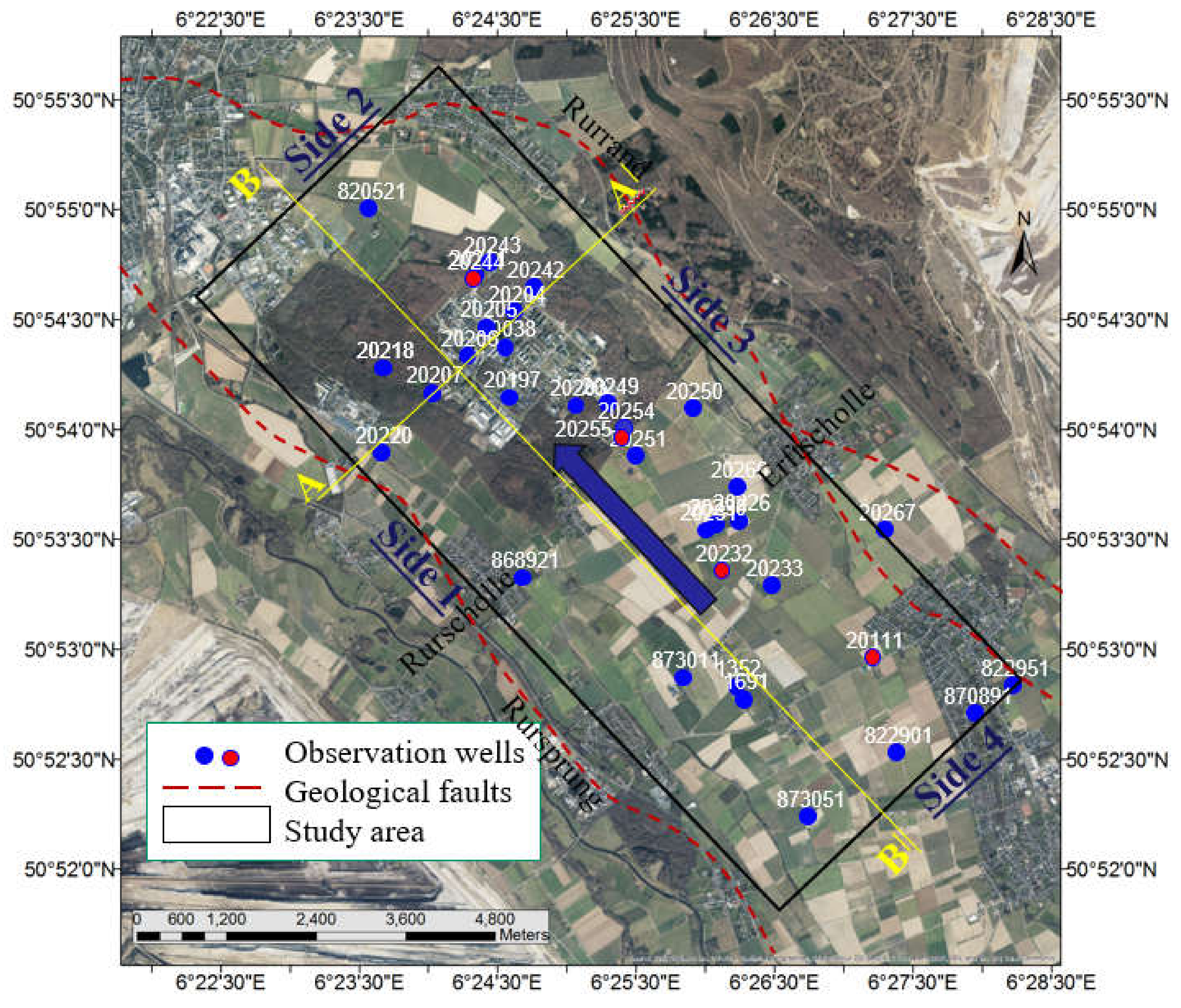
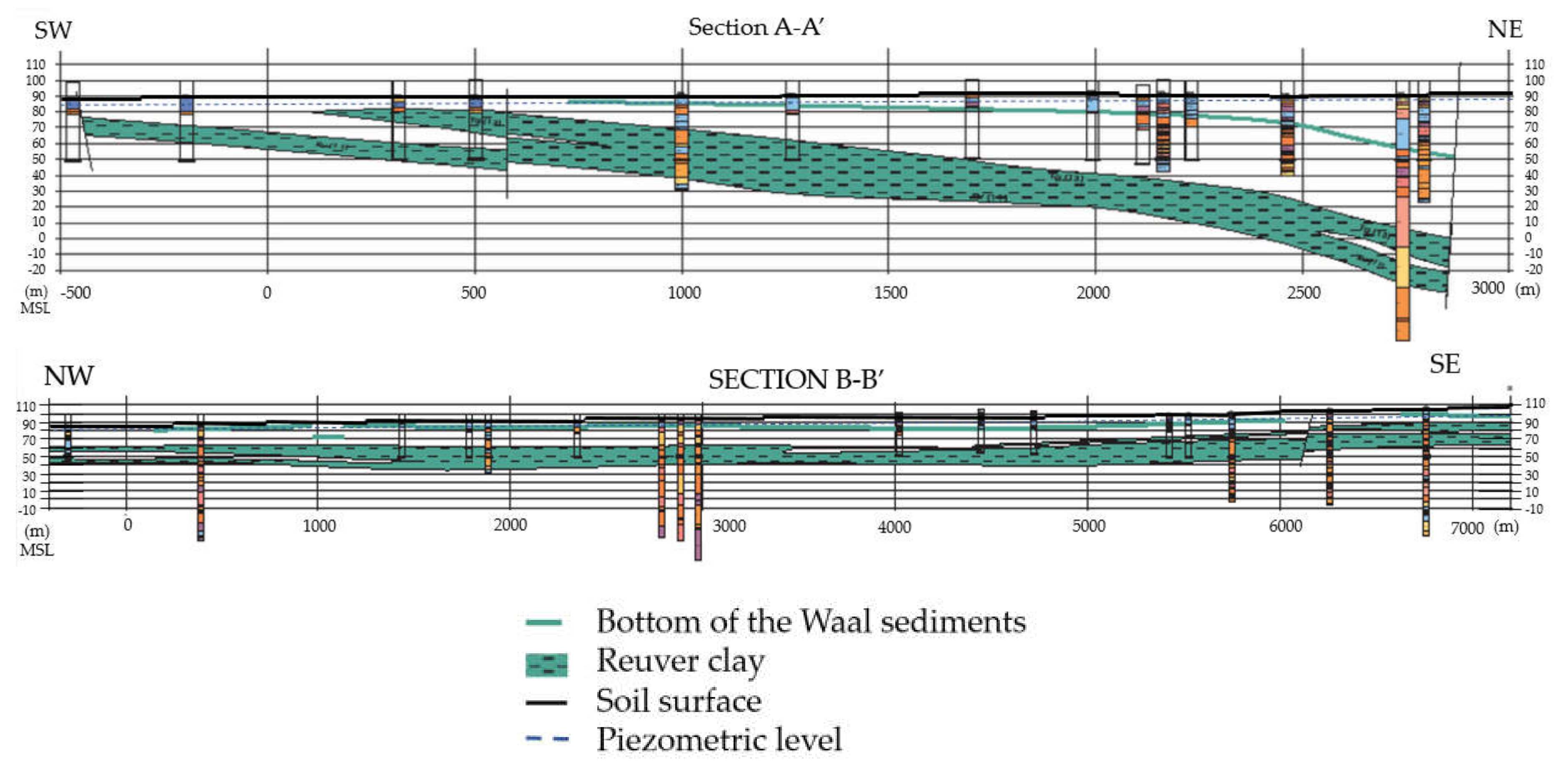
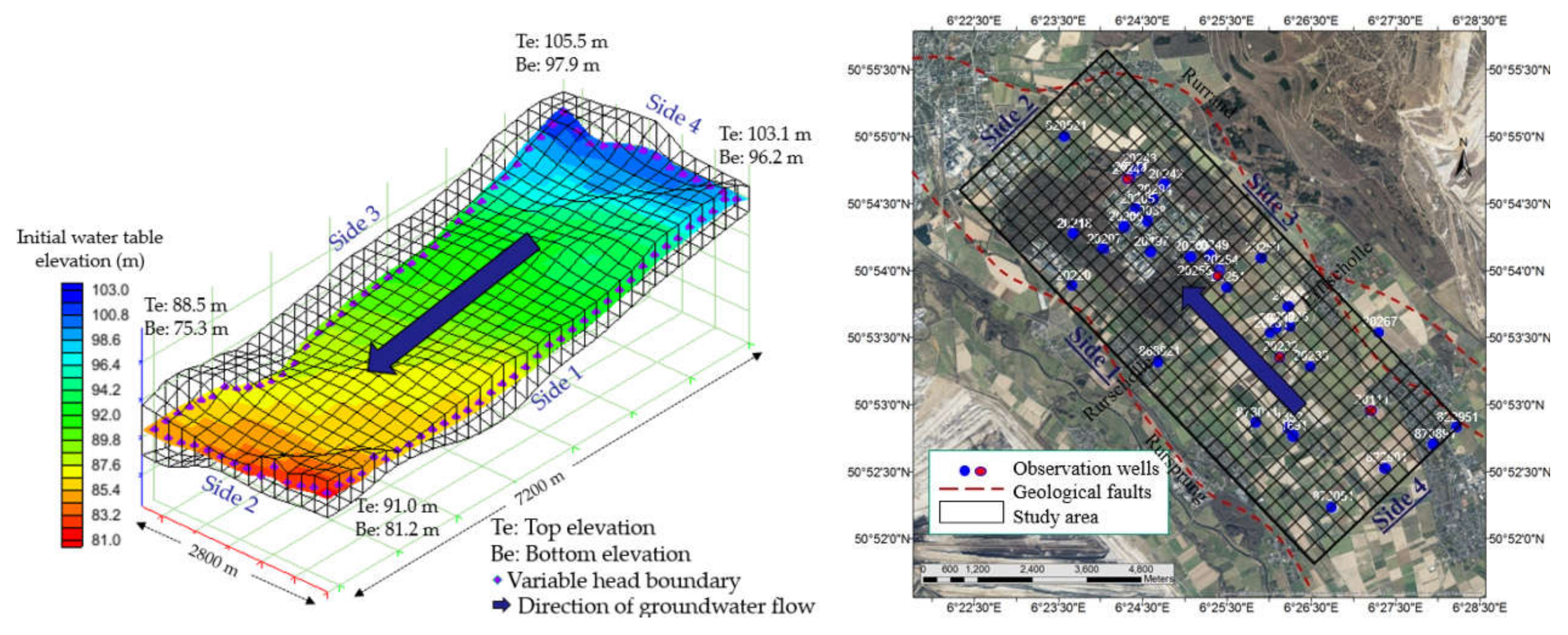
2.1. Study Area: Zwischenscholle Aquifer

The study area, the ‘Zwischenscholle aquifer,’ is located near Jülich in the Lower Rhine Embayment, Germany. The Zwischenscholle aquifer is surrounded by Rurscholle separated by the Rursprung fault in the southwest and by Erftscholle separated by the Rurrand fault in the northeast. The Zwischenscholle area is lower than Erftscholle and higher than Rurscholle. Figure 1 shows the study area with geological faults and observation wells. Forest and agriculture are the major land uses in this area. The western side is characterized by deciduous forest, whereas the eastern part is dominated by agricultural land use [55]. The unconfined or semi-confined aquifer consists of Quaternary Rhine Maas sand and gravel sediments with a Reuver clay aquifer base. The groundwater flow direction is from southeast to northwest (a blue arrow in Figure 1) with a mean hydraulic gradient between 0.1% and 0.2% [56]. The thickness of the aquifer varies from a few meters in the southwest to 35 m in the northeast. Land use, soil type, and soil hydraulic properties in the study area are discussed in detail in Section 2.3.2 and Section 2.3.3. Hydrogeological cross-sections A-A’ and B-B’ of the aquifer are shown in Figure 2. It can be observed that the base of the upper aquifer is closer to the surface in the southwest (a cross-section A-A’). There is an increase in the aquifer thickness in the north-western direction (a cross-section B-B’). The thin green line (the bottom of the Waal sediments in this area) represents the aquifer base considered in the current study. This is obtained from the interpolation of the borehole data [55]. At some locations (e.g., southwest of cross-section A-A’), where the Waal sediment layers were not present, the base of the aquifer is limited to depth with a lower range of hydraulic conductivity. The green surface represents the Reuver clay, which is the aquifer base of a second (deeper) groundwater body. Four sides of the study area are represented in Figure 1 as Sides 1, 2, 3, and 4.

2.2. MODFLOW with the HYDRUS-1D Package and MT3DMS

In MODFLOW with the HYDRUS-1D package [49,57] and MT3DMS [43], the one-dimensional HYDRUS-1D [46] model for water flow and solute transport modeling in the unsaturated zone is linked to MODFLOW [58], a three-dimensional model for water flow modeling of the saturated zone, and loosely coupled to MT3DMS (for solute transport modeling of the saturated zone) [53,54].

The HYDRUS-1D model [59] solves water flow in the unsaturated zone using the modified one-dimensional Richards equation:

$$\frac{\partial \theta }{\partial t}=\frac{\partial }{\partial z}\left[K\left(h\right)\left(\frac{\partial h}{\partial z}+1\right)\right]-S\left(h\right)$$

(1)

where θ is the volumetric water content (dimensionless), h is the soil water pressure head (L), t is time (T), z is the vertical coordinate (L) (positive upward), S is the sink term (T⁻¹), and K(h) is the unsaturated hydraulic conductivity (LT⁻¹).

HYDRUS-1D additionally simulates solute transport in variably saturated porous media using the standard advection-dispersion transport equation of the form:

$$\frac{\partial \theta c}{\partial t}+{\rho }_b\frac{\partial s}{\partial t}=\frac{\partial }{\partial z}\left(\theta D\frac{\partial c}{\partial z}\right)-\frac{\partial qc}{\partial z}-\varnothing$$

(2)

where c is the solution concentration (ML⁻³), s is the sorbed concentration (MM⁻¹), D is the dispersion coefficient (L²T⁻¹), 𝜌_b is the bulk density of the porous medium (ML⁻³), q is the volumetric flux density (LT⁻¹), which is obtained using the Darcy–Buckingham law, and $\varnothing$ is a sink–source term accounting for various zero- and first-order or other reactions (ML⁻³T⁻¹) [60]. In the current study, atrazine is considered to undergo the first-order degradation. Therefore,

$$\varnothing =\lambda \left(\theta c+{\rho }_{b}S\right)$$

(3)

where λ is the first-order degradation rate (day⁻¹). Root solute uptake is not considered in this study.

In MODFLOW, the three-dimensional movement of groundwater of a constant density is described by the following partial differential equation:

$$\frac{\partial }{\partial x}\left(K_{xx}\frac{\partial h}{\partial x}\right)+\frac{\partial }{\partial y}\left(K_{yy}\frac{\partial h}{\partial y}\right)+\frac{\partial }{\partial z}\left(K_{zz}\frac{\partial h}{\partial z}\right)+w=S_s\frac{\partial h}{\partial t}$$

(4)

where K_xx, K_yy, and K_zz are values of the hydraulic conductivity along the x, y, and z coordinate axes, which are assumed to be parallel to the major axes of hydraulic conductivity (LT⁻¹), h is the potentiometric head (L), W is a volumetric flux per unit volume representing sources and/or sinks of water (T⁻¹), S_S is the specific storage of the porous material (L⁻¹), and t is time (T).

MT3DMS simulate advection, dispersion/diffusion, and chemical reactions of contaminants in the saturated zone using the following partial differential equation:

$$\frac{\partial \left(\theta c\right)}{\partial t}=\frac{\partial }{\partial x_i}\left(\theta D_{ij}\frac{\partial c}{\partial x_j}\right)-\frac{\partial }{\partial x_i}\left(\theta v_{i}c\right)+q_s{c}_s+\sum R_n$$

(5)

where c is the dissolved solute concentration (ML⁻³), θ is the porosity of the subsurface medium (dimensionless), t is time (T), x_i is the distance along the respective Cartesian coordinate axis (L), D_ij is the hydrodynamic dispersion coefficient tensor (L²T⁻¹), v_i is the pore water velocity (LT⁻¹), q_s is the volumetric flow rate per unit volume of the aquifer representing fluid sources (positive) and sinks (negative) (T⁻¹), c_s is the concentration of the source or sink flux (ML⁻³), and $\sum R_n$ is the chemical reaction term (ML⁻³T⁻¹).

In MODFLOW, the groundwater domain is discretized into finite difference grids. These grids are then combined into multiple zones based on the similarities in soil characteristics, topographical characteristics, boundary conditions, and the depth to groundwater. Each of these zones is then assigned one soil profile that extends from the soil surface down to a depth, which should be below the deepest possible water table level that can occur during the simulation (hereafter referred to as the ‘HYDRUS-1D profile’). The entire period of simulation in MODFLOW is divided into stress periods, during which the input data for all external stresses (e.g., rainfall, potential evapotranspiration, pumping, recharge, etc.) are constant. These stress periods are further divided into time steps. Time steps are intervals in each stress period, during which the change in the aquifer characteristics (e.g., groundwater head/water table level, groundwater flow, etc.) due to external stresses is analyzed using the model. Water flow and solute transport are simulated in each HYDRUS-1D profile for a duration equal to one MODFLOW time step by considering the average water table level from MODFLOW as the bottom pressure head boundary condition. The time-averaged bottom flux from the HYDRUS-1D profile is given as the recharge flux to MODFLOW, which then simulates groundwater flow. The average water table depth at the end of the MODFLOW time step is assigned as the bottom pressure head boundary condition in the HYDRUS-1D profile for the next MODFLOW time step [49,53,54,57]. The solute flux reaching the water table is further used for solute transport modeling in the saturated soil zone using MT3DMS.

2.3. Data Available for Modeling

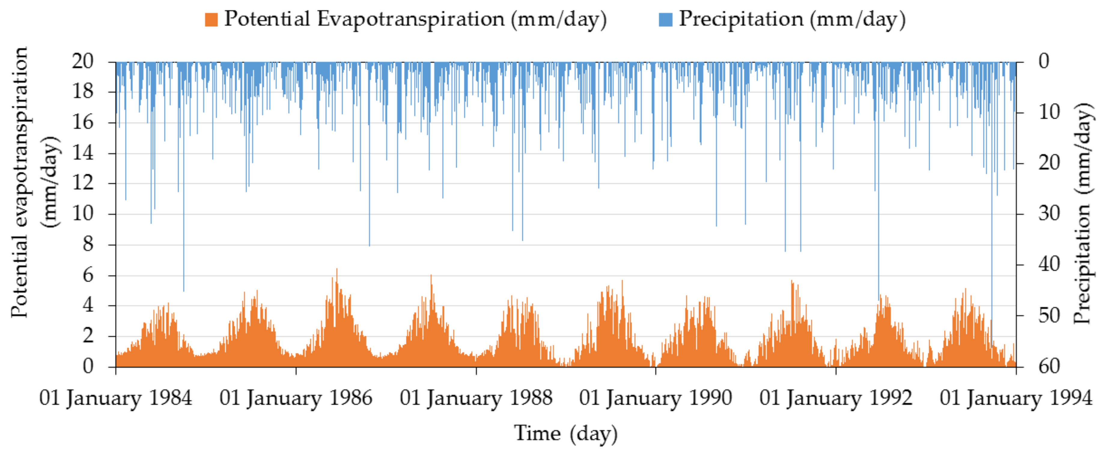
Aquifer data available for modeling and model validation include (i) information about precipitation, potential evapotranspiration, boundary conditions, land use, and approximate amounts of atrazine applied in agricultural fields from 1984 to 1993, (ii) atrazine concentrations in different observation wells in 1991, 1992, and from 2000 to 2011, except for the year 2004 [20,21], and (iii) water table fluctuations in selected observation wells in the study area from 1984 to 1993. The information about land use and approximate quantities of atrazine applied in maize fields was obtained using a questionnaire survey from the farmers [61]. Exact locations of maize fields and quantities of atrazine applied over the years in the study area are unknown since this information was not recorded [61]. Therefore, the modeling is based on scenarios of atrazine applications that are realistic in a statistical sense.

2.3.1. Climate Data

The climate data were obtained from the meteorological tower installed in the Jülich Research Centre [30]. Precipitation and potential evapotranspiration, calculated using the Penman–Monteith equation, from 1984 to 1993 are shown in Figure 3.

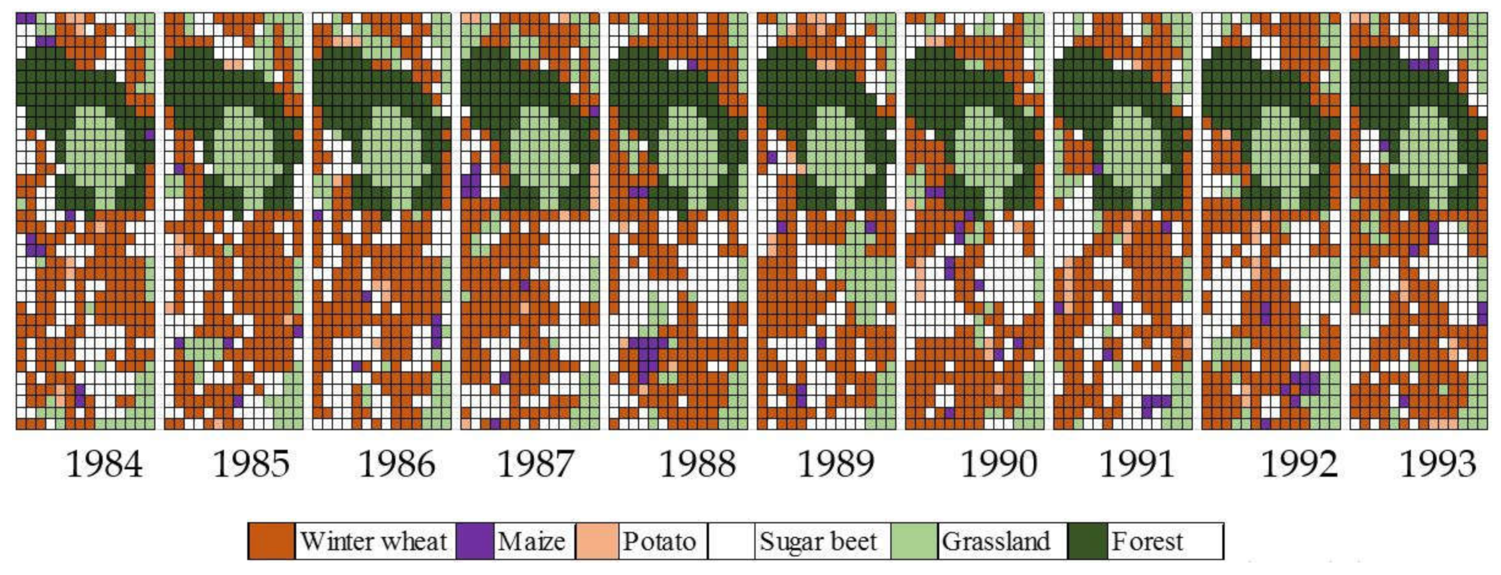
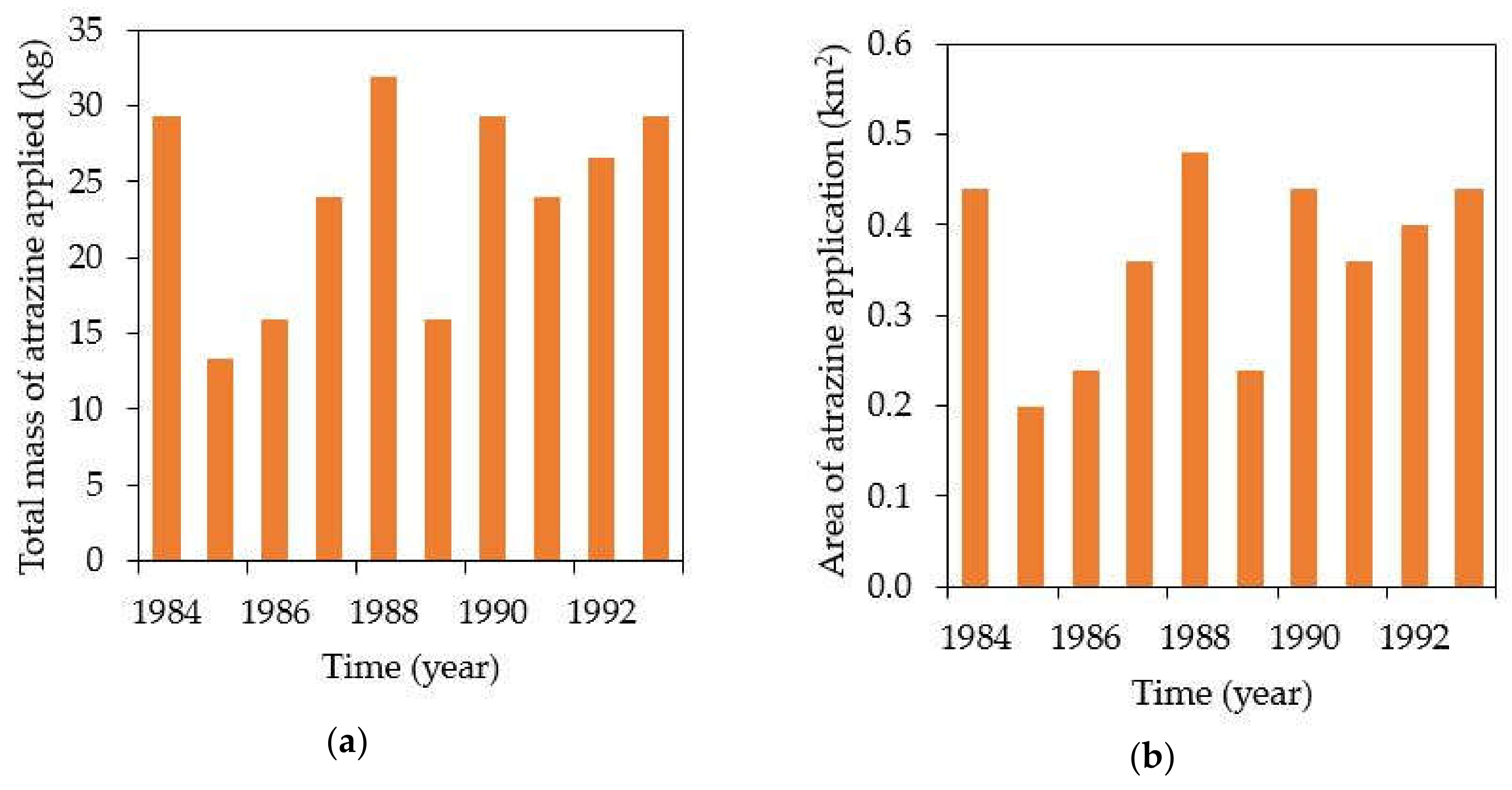
2.3.2. Land Use and Information about Atrazine Applications

The primary land use is agriculture. Since a complete map of land use was not available, a stochastic distribution approach was used to generate possible hypothetical land use [30]. Figure 4 shows the spatial distribution of different land uses from 1984 to 1993. Winter wheat, sugar beet, pasture, maize, and potatoes represent about 50%, 35%, 8%, 4%, and 3%, respectively, of the total agricultural land. The total area of maize fields is significantly smaller compared to other crops and is highly spatially spread in the study area.

The average application rate of atrazine in the agricultural field cultivated with maize is 0.0666 g/m² [61]. Atrazine was applied once a year around May. Figure 5 shows the total mass of atrazine applied in the study area and the area of the atrazine application from 1984 to 1993 [61].

2.3.3. Soil Types and Soil Hydraulic Properties

The study area is characterized by loess sediments. Details regarding different soil types and soil layers were available for the study area from the Forschungszentrum Jülich GmbH (as a part of the MOSYRUR project [61], a project analyzing the water balance in the Rur basin). Soils in the study area are classified into four soil types (silt loam, sandy loam, loam 1, and loam 2) and the parameters of the van Genuchten–Mualem soil hydraulic functions [62] were derived for different layers of the four soil types.

Table 1. Different types of soil, soil layers, soil hydraulic properties (the van Genuchten–Mualem analytical model parameters) [62] and aquifer properties [30,61].

Soil Type	Layers	Thickness (m)	Residual Water Content, θr (-)	Saturated Water Content, θs (-)	Parameter α in the Soil Water Retention Function, (m−1)	Parameter n in the Soil Water Retention Function, (-)	Saturated Hydraulic Conductivity, Ks (m day−1)	Tortuosity Parameter l in the Conductivity Function (-)
Silt loam	1	0.23	0.045	0.463	2.16	1.35	0.080	0.5
	2	0.28	0.041	0.392	1.60	1.35	0.032	0.5
	3	1.35	0.074	0.359	1.42	1.30	0.017	0.5
Sandy loam	1	0.25	0.056	0.382	11.2	1.35	1.38	0.5
	2	0.30	0.053	0.314	9.33	1.40	0.891	0.5
Loam 1	1	0.06	0.048	0.461	2.10	1.34	0.074	0.5
	2	1.00	0.082	0.358	4.32	1.33	0.067	0.5
Loam 2	1	0.20	0.044	0.395	2.04	1.34	0.049	0.5
	2	1.00	0.069	0.298	4.16	1.33	0.110	0.5
Aquifer	-	Variable	0.001	0.184	10.0	2.10	134.	0.5

shows the details about various soil types, soil layers, soil hydraulic properties (van Genuchten–Mualem analytical model parameters), and aquifer properties.

2.3.4. Simulation of Crop Transpiration and Root Water Uptake

The plant module SUCROS [63] was used by Herbst et al. [30] to estimate temporal changes in the leaf area index (LAI) of various crops in the study area. The crop coefficient (K_c) is used to derive specific crop evapotranspiration from potential reference evapotranspiration using the equation: ET_crop = ET_pot K_C, where ET_pot (LT⁻¹) is potential evapotranspiration for the reference grass cover, ET_crop (LT⁻¹) is plant-specific potential evapotranspiration. Temporal changes in the crop K_c factor followed the Doorenbos and Pruitt [64] approach [61]. Actual transpiration from the soil is estimated in the HYDRUS-1D package based on root water uptake characteristics. In HYDRUS-1D, root water uptake is represented as extraction or a sink term distributed over the root zone. Root water uptake is evaluated using potential transpiration and the Feddes stress response function [65]. Parameters of the Feddes stress response function used for different crops are given in

Table 2. The Feddes stress response function parameters and maximum rooting depths of different crops (P0 is the pressure head, below which roots start extracting water from the soil, POpt is the pressure head, below which roots extract water at the maximum possible rate, P2H is the value of the limiting pressure head, below which roots can no longer extract water at the maximum rate of 0.5 cm/day, P2L is the value of the limiting pressure head, below which roots can no longer extract water at the maximum rate of 0.1 cm/day, and P3 is the pressure head, below which root water uptake ceases).

Crop	P0 (m)	POpt (m)	P2H (m)	P2L (m)	P3 (m)	Maximum Rooting Depth (m)
Winter wheat	0.000	−0.010	−5.00	−9	−160	0.95
Maize	−0.150	−0.300	−3.25	−6	−80	1.15
Potato	−0.100	−0.250	−3.20	−6	−160	0.74
Sugar beet	−0.100	−0.250	−3.20	−6	−160	1.15
Grassland	−0.001	−0.025	−2.00	−8	−80	0.75
Forest	1000.001	1000	−4.25	−8	−160	1.50

. Rooting depths and root densities of various crops grown in the study area are given in

Table 3. Relative rooting depths and root densities of different crops [55].

Relative Rooting Depth (-)	Root Density; Value Characterizing the Depth Distribution of Root Water Uptake (m−1)
	Winter Wheat	Maize	Potato	Sugar Beet	Grassland	Forest
0.0	0.26	1.05	1.00	0.97	1.05	0.30
0.1	0.16	0.76	0.94	0.92	0.76	0.60
0.2	0.10	0.55	0.89	0.86	0.55	0.90
0.3	0.06	0.39	0.84	0.80	0.39	0.95
0.4	0.04	0.28	0.78	0.74	0.28	0.90
0.5	0.02	0.20	0.73	0.69	0.20	0.80
0.6	0.01	0.15	0.68	0.63	0.15	0.70
0.7	0.01	0.10	0.62	0.57	0.10	0.60
0.8	0.00	0.07	0.57	0.51	0.07	0.50
0.9	0.00	0.05	0.52	0.46	0.05	0.40
1.0	0.00	0.04	0.47	0.40	0.04	0.30

.

2.3.5. Solute Transport Parameters

Solute transport is described using the advection-dispersion equation. A linear sorption isotherm is used to describe the sorption of atrazine. The sorption constant K_d (m³/kg), the first-order degradation rate, λ (day⁻¹), the bulk density (kg/m³), and the longitudinal α_L (m) and transverse α_T (m) dispersivities for different soil types and soil depths are given in

Table 4. Solute transport parameters specific to soil and solute [55].

Soil Type	Layers	Porosity (-)	Longitudinal Dispersivity, αL (m)	Transverse Dispersivity, αT (m)	Bulk Density, (kg/m3)	Adsorption Coefficient, Kd (m3/kg)	First-order Degradation Rate, λ (day−1)
Silt loam	1	0.509	0.045	0.0045	1350	1.42 × 10−3	3.47 × 10−3
	2	0.434	0.045	0.0045	1375	3.26 × 10−4	1.73 × 10−3
	3	0.434	0.045	0.0045	1375	1.63 × 10−4	1.04 × 10−3
Sandy loam	1	0.509	0.045	0.0045	1350	1.42 × 10−3	3.47 × 10−3
	2	0.434	0.045	0.0045	1375	3.26 × 10−4	1.73 × 10−3
Loam 1	1	0.510	0.045	0.0045	1350	6.91 × 10−3	3.47 × 10−3
	2	0.440	0.045	0.0045	1375	6.52 × 10−4	1.73 × 10−3
Loam 2	1	0.509	0.045	0.0045	1350	1.42 × 10−3	3.47 × 10−3
	2	0.434	0.045	0.0045	1375	3.26 × 10−4	1.04 × 10−3
Aquifer	-	0.184	15.4	1.54	1400	3.55 × 10−4	3.47 × 10−10

. It can be noted that the first-order degradation rate in the aquifer is very low (3.47 × 10^-10 day⁻¹) [55], which could be the main reason for the long-term stable atrazine concentration in the groundwater [20,21].

2.4. Model Setup

2.4.1. Spatial and Temporal Discretizations

The study area of 21 km² was divided into 504 MODFLOW grids each of a dimension of 200 × 200 m (14 columns and 36 rows). Figure 6 shows the initial water table elevation, MODFLOW grids, boundary conditions, the groundwater flow direction, and the top and bottom elevations of the aquifer at four boundary points. Considering the highly variable soil hydraulic properties, surface elevations, water table elevations, and atmospheric boundary conditions in the study area, each MODFLOW grid cell was assigned a single HYDRUS-1D profile. The top elevation of the HYDRUS-1D profile was considered as the surface elevation corresponding to the MODFLOW grid cell assigned to the profile. The bottom elevation of each HYDRUS-1D profile was set 2 m below the initial water table elevation in the grid cell. This was further adjusted by performing trial runs that checked for the possibility of the water table falling below the bottom of the HYDRUS-1D profile. Each HYDRUS-1D profile was then divided into finite elements based on the soil hydraulic properties and the depth of the HYDRUS-1D profile. The ratio of the sizes of neighboring finite elements was always less than 1.5 to ensure the convergence of the solution. The total number of finite elements varied from 150 to 250 in all profiles. The number of stress periods and time steps used in this study is 14,609, with the duration of each time step equal to 1 day. The functioning of the model is explained in Section 2.2.

2.4.2. Initial and Boundary Conditions

The water table elevation in the year 1984 (the beginning of the simulation) obtained by interpolating groundwater table levels in the observation wells in the study area [61] was given as the initial water table elevation (Figure 6). The atmospheric boundary condition was given at the surface using precipitation and potential evapotranspiration fluxes. A no-flow boundary condition was assumed at the bottom of the aquifer. Ten layers were considered for groundwater modeling using MODFLOW and solute transport modeling using MT3DMS. The monthly varying water table levels were given as the variable head boundary conditions on all lateral boundaries of the study domain. This data was obtained using a spatiotemporal interpolation procedure for defining the heads at the boundary at a 30-day time step from the measured groundwater levels in the aquifer [30].

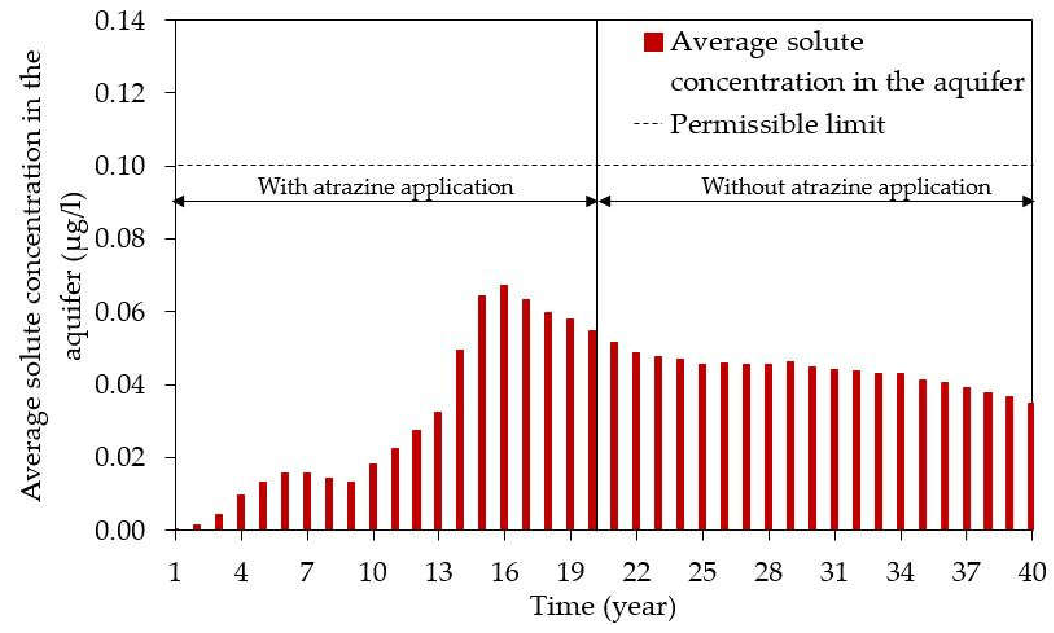
2.4.3. Model Settings for Analyzing the Long-Term Atrazine Concentrations in Groundwater

To simulate the long-term atrazine concentrations in groundwater and also to validate the model, the simulation period was extended until 2023. All information (precipitation, potential evapotranspiration, boundary conditions, and land use), available for the first 10 years (1984–1993), was repeated three times (from 1994 to 2023) during this exercise. This approach was used because the data needed for the boundary conditions (the spatially and temporally interpolated groundwater table levels) and land use were not available for the period after 1993. A similar approach was adopted by Rakowski et al. [66] for developing future scenarios in groundwater modeling. The information regarding precipitation and potential evapotranspiration from 1994 to 2023 could have been obtained either from the weather station in the study area or using weather forecasting. However, since water table levels that could be used as boundary conditions were not available for this period, and also since these water table levels depend on precipitation, it was decided to repeat the information. During the 40-year simulation period, atrazine was applied during the first 20 years. The evolution of atrazine concentrations during the first 20 years represents the change of atrazine concentrations over time after the use of a substance in a certain region started. The last 20 years of the simulation represent how the concentrations decrease after a ban on atrazine.

2.4.4. Looping Boundary Condition

Since there is no specific information available regarding the inflow of solute with groundwater across the lateral boundaries of the study domain, a methodology was developed in this study to represent the effects of the entire basin on the study area (a part of the basin). Instead of considering the inflow of clean water (water without atrazine) through the lateral aquifer boundaries, solute concentrations from MODFLOW cells in the layers which are saturated at the outflow side of the domain were used in the corresponding active cells at the inflow side of the domain. This is further referred to as a ‘looping boundary condition.’ In this case study, the looping boundary condition was considered only in the main direction of groundwater flow, which is from south-east to north-west (from Side 4 to Side 2 in Figure 1). This boundary condition assumes that the average atrazine concentration in water that percolates from the saturated soil zone to the downstream aquifer in the study domain is equal to the average concentration of atrazine that reaches the groundwater in the upstream part of the aquifer. Note that the use of this looping concentration boundary condition does not prevent the atrazine mass in the aquifer to decrease over time. Due to incoming recharge, outgoing water and atrazine fluxes are larger than incoming fluxes, and thus the total atrazine mass in the aquifer decreases over time when recharge does not any longer contain atrazine (due to its ban). The source code of MT3DMS (http://hydro.geo.ua.edu/mt3d) was modified to incorporate this special boundary condition.

3. Results and Discussion

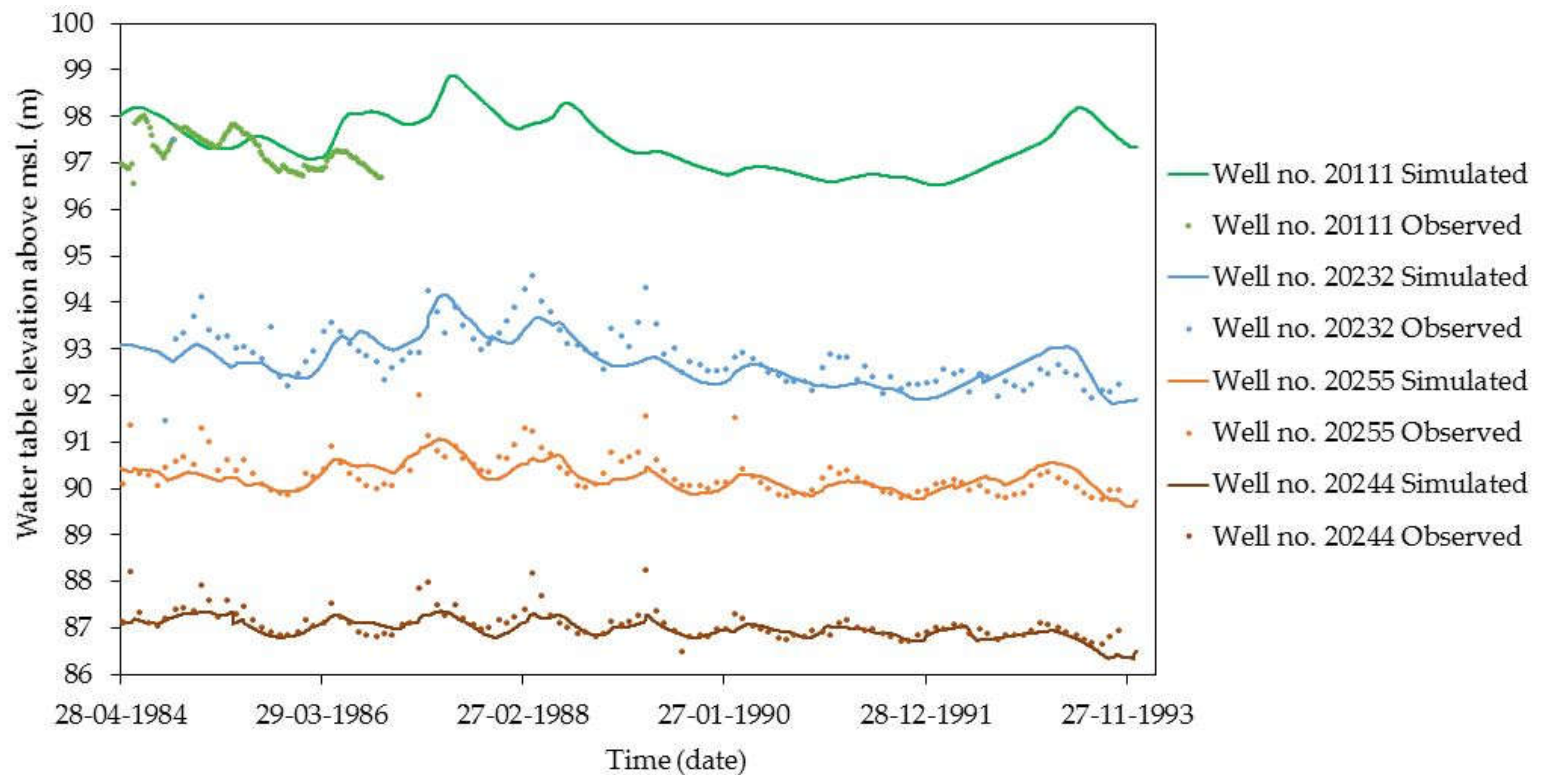
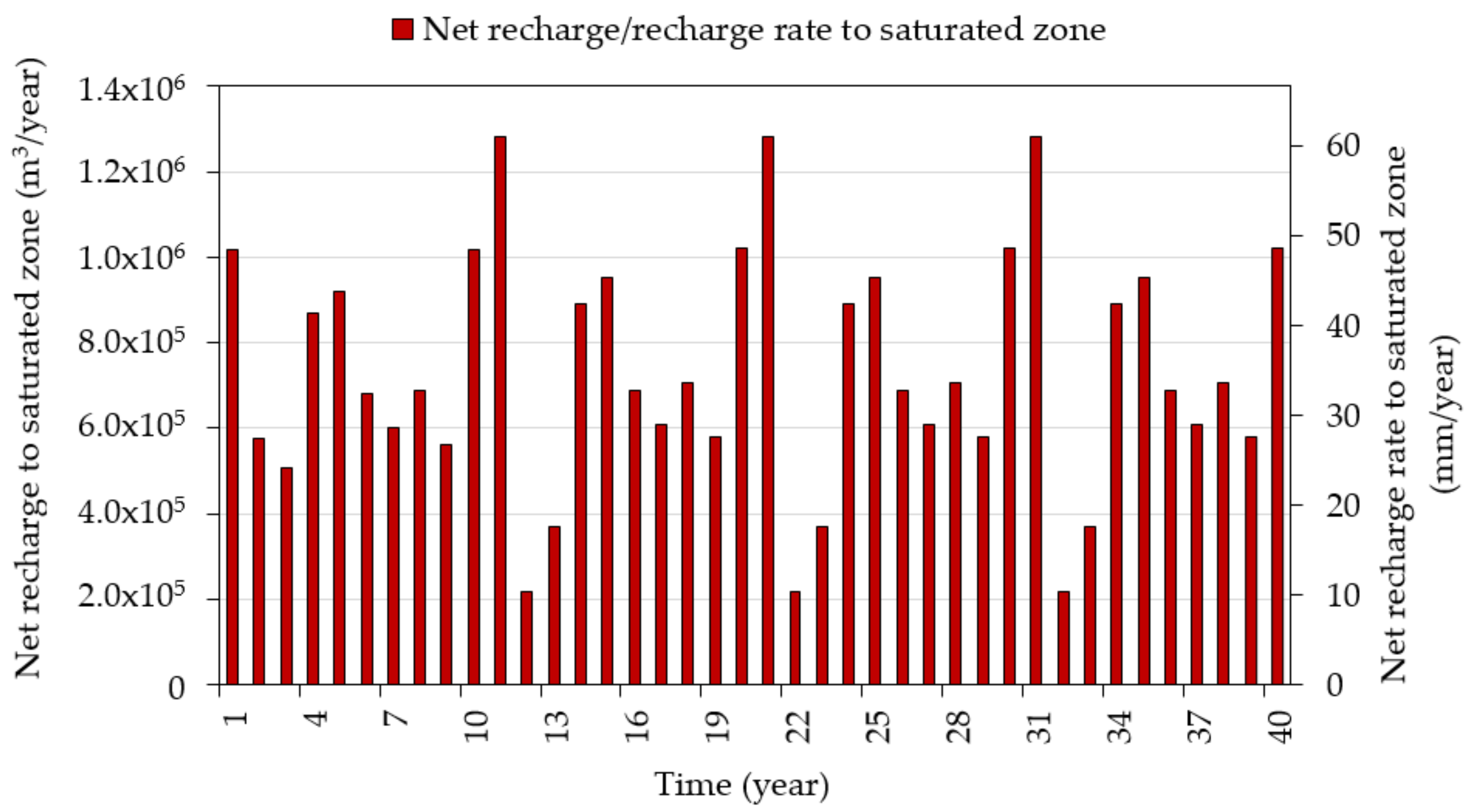
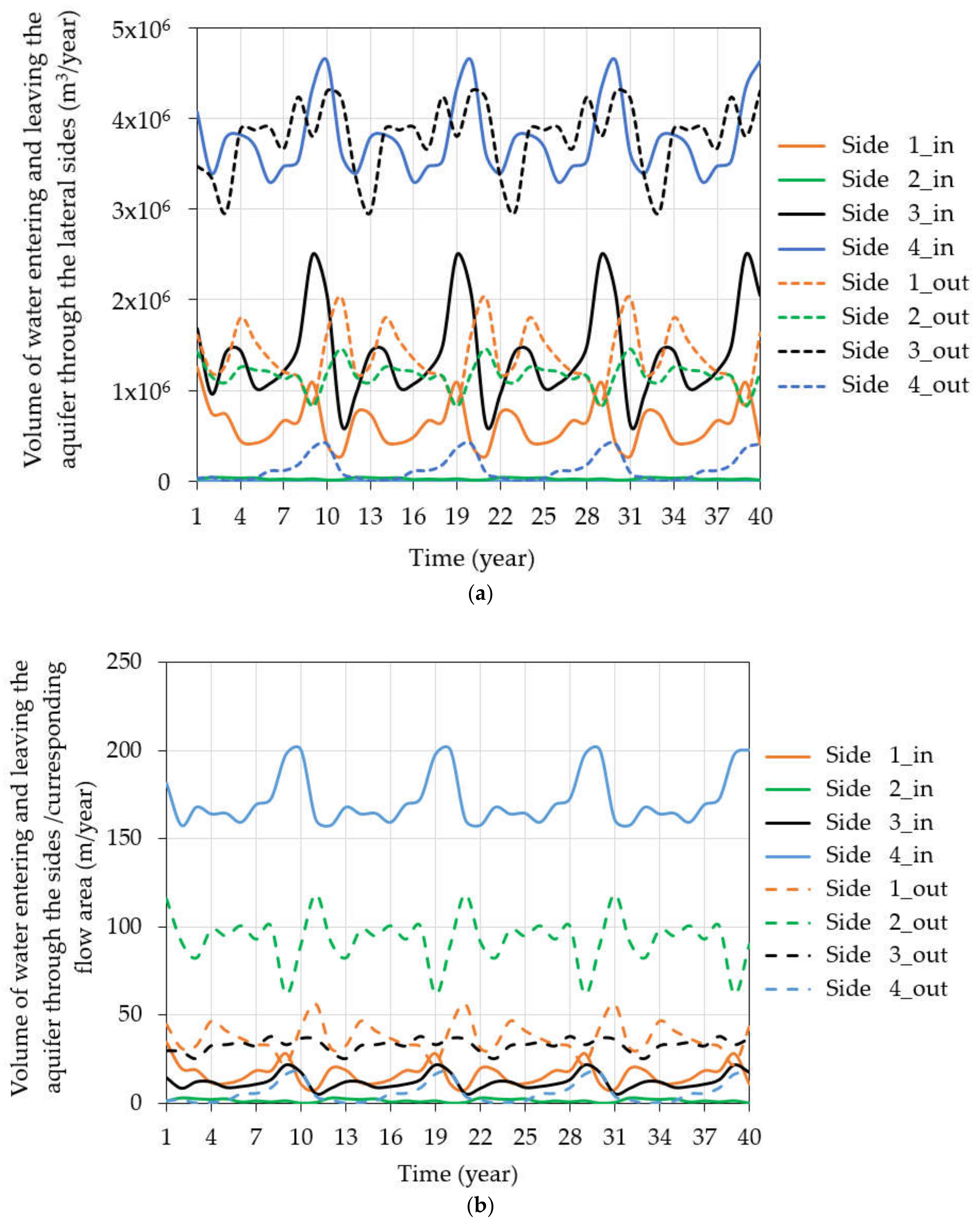
3.1. Water Flow Modeling Using MODFLOW with the HYDRUS-1D Package

Figure 1 shows several observation wells in the study area represented by well identification numbers. These are the wells, in which water elevations and atrazine concentrations were monitored [30]. Since there are only a few wells with information regarding the water table elevation with a high temporal resolution, only four observation wells highlighted in red color (well numbers 20232, 20111, 20244, and 20255 in Figure 1) were used for model validation. The water table elevation data is available from October 1984 to November 1993, December 1983 to October 1986, December 1983 to November 1993, and December 1983 to November 1993 for wells 20232, 20111, 20244, and 20255, respectively.

Figure 7 shows the comparison of model-simulated and observed water table elevations in the study area. In general, observed and simulated water table elevations are found to be similar in all four observation wells. Minor differences between observed and simulated water table elevations could be the result of comparing observed point data with the average simulated water table position in the grid cell (the grid cell area of 40,000 m² in this study). Another plausible reason for the anomaly between simulated and observed water tables could be the fact that the boundary condition provided to the model was generated by spatiotemporal interpolation [30], which may also exhibit a certain level of inaccuracy. Furthermore, the aquifer properties (hydraulic conductivity, specific yield, and porosity) may vary spatially. Additionally, a constant value of the specific yield was used in the groundwater model simulations in the developed model. The specific yield can be considered constant only when the aquifer response is linear, i.e., when the volume of water added or released is linearly proportional to the water table fluctuation. The specific yield varies based on the transient nature of the water release from the unsaturated soil zone, soil hydraulic properties, the depth to the groundwater table, or hysteresis [67,68], which are factors not taken into account in this study.

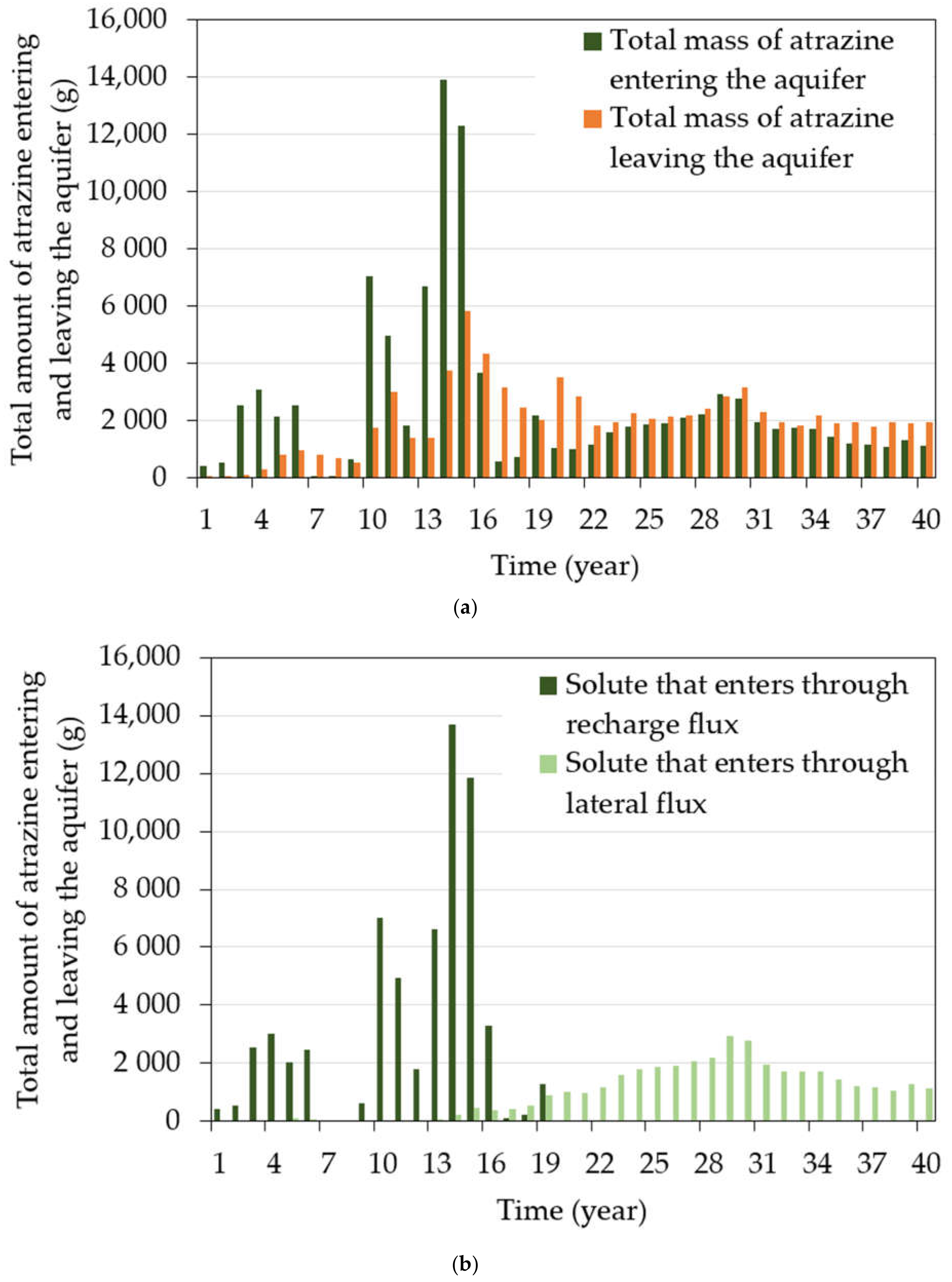
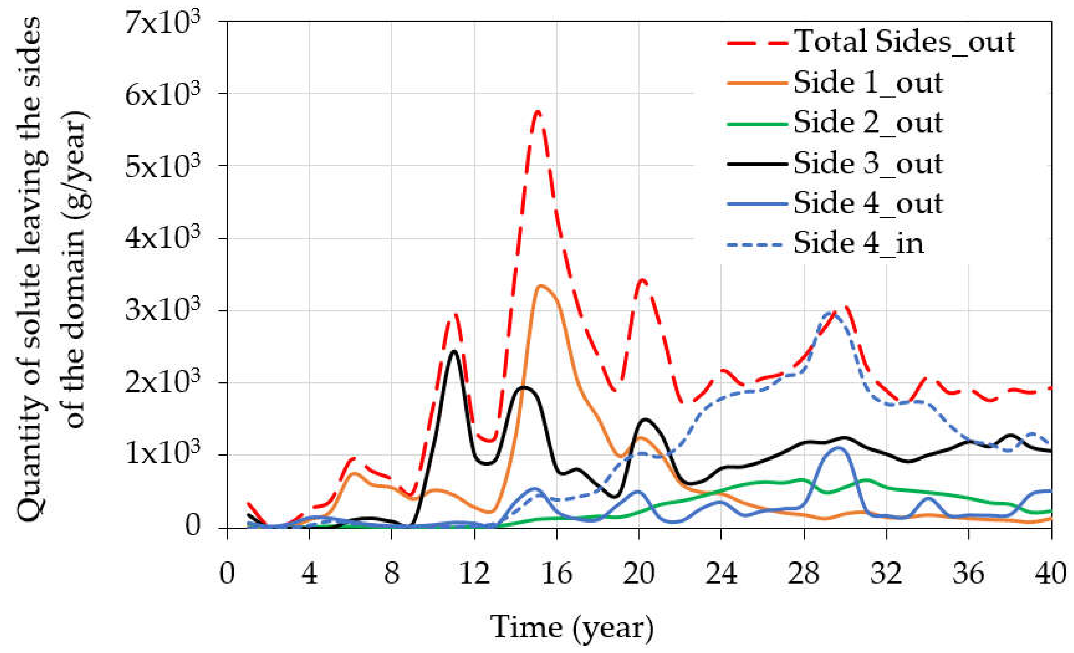
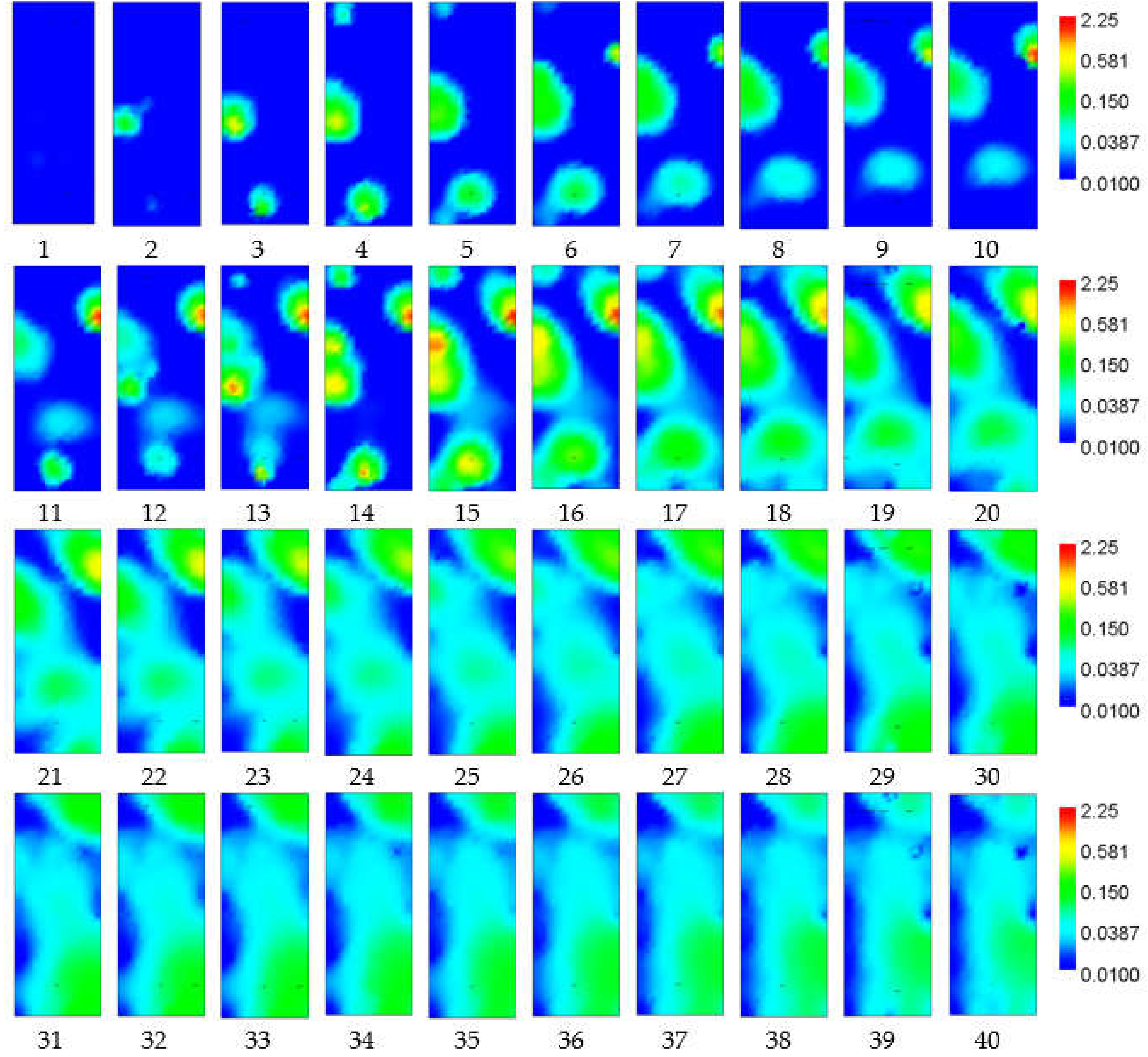
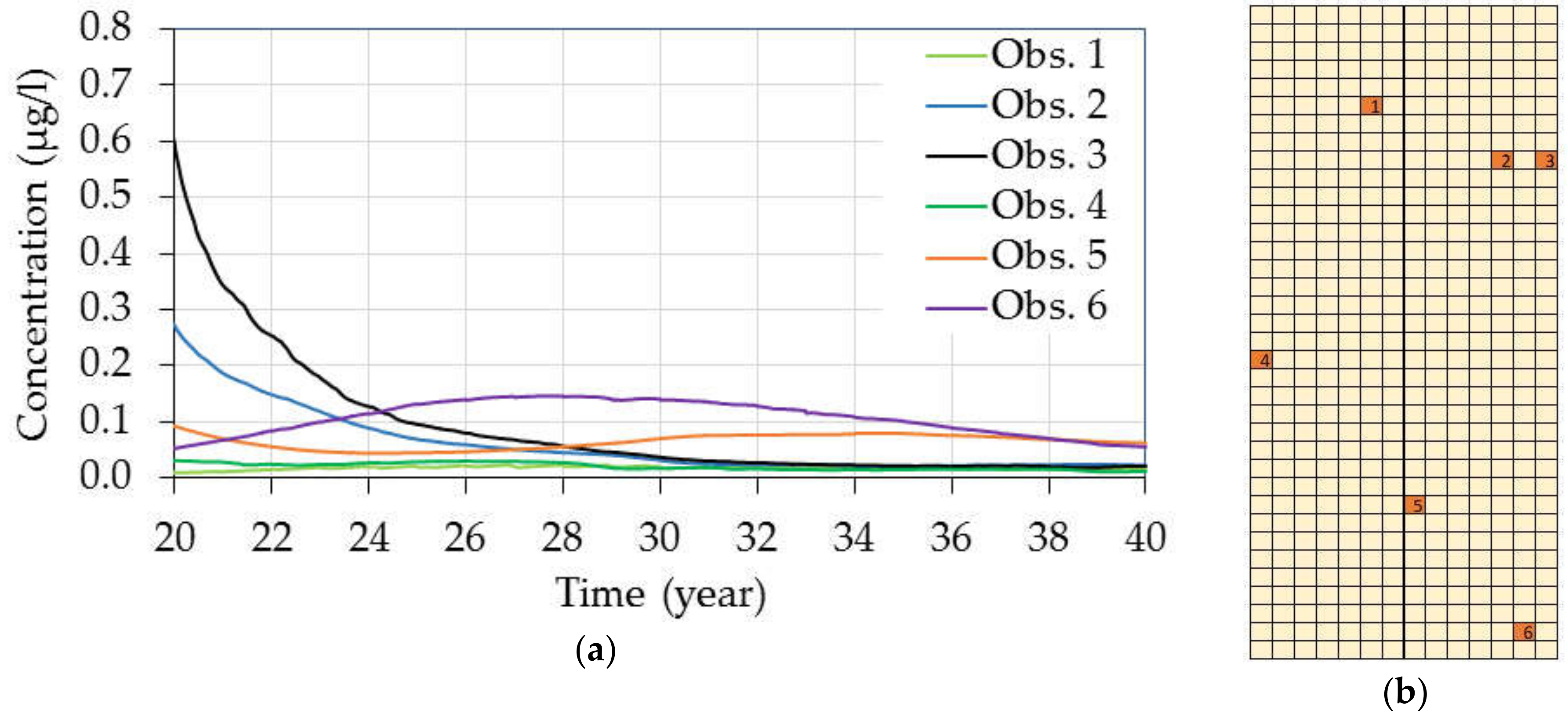
3.2. Atrazine Concentrations in Groundwater

Figure 8 shows the average annual atrazine concentration in the groundwater obtained using MODFLOW with the HYDRUS-1D package and MT3DMS. The horizontal dotted line shows the permissible limit of atrazine concentrations, and the vertical line indicates the period when atrazine applications in the field stopped. The atrazine concentration appeared in the groundwater about one year after the start of its use. The atrazine concentration in the aquifer increased during the period of its application and started slowly decreasing once its application was stopped. The rate at which the average solute concentration is increasing/decreasing in the aquifer depends on the rate of recharge from the unsaturated soil zone to the saturated soil zone, the rate of atrazine application, the location of the maize fields, lateral groundwater flow into and out of the saturated soil zone, and the looping boundary condition.

Figure 9 shows total net recharge (in m³/year) and the net recharge rate (in mm/year) between the unsaturated and saturated soil zones in each year. Recharge depends on atmospheric boundary conditions (precipitation, potential evaporation), land use, and soil hydraulic properties. It can be observed that the net recharge varies from year to year, with a maximum rate of about 61 mm/year and a minimum rate of about 11 mm/year.

Figure 10a shows the total inflow and outflow of water through the four lateral sides of the aquifer. The amounts of water leaving and entering through the four lateral sides (Side 1 to Side 4 in Figure 1) are different because of groundwater gradients and differences in flow areas of each of these sides. The maximum flow area is on Side 3, followed by Sides 1, 4, and 2. Most water is flowing into the domain through Side 4 (Side 4_in), and most water is leaving the aquifer through Side 3 (Side 3_out). In the looping direction (Sides 2–Side 4), more water is entering the domain through Side 4 than leaving through Side 2. Figure 10b shows volumes of water entering and leaving the aquifer through four lateral sides divided by corresponding flow areas (area through which flux goes in or out), which represents average water fluxes. It can be observed that the relative volume (for the flow area) of water entering the aquifer is highest on Side 4 (Side 4_in) and lowest on Side 2, while the relative volume of water leaving the aquifer is highest on Side 2 (Side 2_out) and lowest on Side 4 (Side 4_out). This indicates that the major flow direction is from (Side 4) south-east to (Side 2) north-west, and the same direction is chosen for the solute transport looping boundary, as explained in Section 2.4.

Figure 11a shows the total amount of atrazine entering the groundwater through various sources and leaving though various sinks. Various sources that add solute into the system include recharge from the unsaturated zone to the saturated zone and lateral inflow through Side 4 (due to the looping boundary condition). Lateral outflow from the aquifer acts as a sink. There was an increase in the total amount of atrazine entering the saturated soil zone from year 3 to year 6 and from year 10 to year 15 (Figure 11). This is because of an increase in the area of the atrazine application and also due to leaching of adsorbed atrazine. There was a decrease in the amount of atrazine reaching the groundwater from year 7 to year 9 and after year 16. This is because of a decrease in the quantity of applied atrazine and the reduction in recharge (Figure 9) during these periods. There was again an increase in the amount of atrazine entering groundwater from year 22 to year 30 and a decrease afterwards. This is because of the looping boundary condition to represent the influx of atrazine from upstream areas.

Figure 11b shows the total mass of atrazine that is entering the aquifer through lateral flux (Side 4) and recharge flux. Large amounts of atrazine are entering the domain through recharge during the first 20 years (when atrazine was applied in the area). When comparing Figure 11a,b, it can be observed that the amount of atrazine entering the aquifer through lateral sides is smaller than the amount of atrazine leaving the aquifer through lateral sides during the first 12 years. This is because of the looping boundary condition and can be explained by Figure 12. Figure 12 shows the amount of atrazine leaving and entering through lateral sides. From Figure 12, it can be observed that only small amounts of atrazine are leaving through Side 2 (Side 2_out) during the first 12 years. Since the looping boundary is considered from Side 2 to Side 4, the amount of atrazine entering the lateral side (Side 4) is also small during this period. During later years (after 12 years) the amount of atrazine leaving through Side 2 increases, and so is the inflow through Side 4 in Figure 12.

From Figure 12, it can be observed that the amount of atrazine leaving through Sides 1 and 3 is higher than through Side 2 in most years. This is because higher volumes of water are leaving through Sides 1 and 3 and also due to the location of atrazine applications. It can also be observed that the amount of solute leaving through Side 3 is always higher than through Side 2 and that the amount of solute entering through Side 4 due to the looping boundary condition corresponds to the amount of solute leaving the aquifer through Side 2. However, the amounts entering via Side 4 are larger than the amount that leaves Side 2 because of the larger water flow into Side 4 than out of Side 2 (see Figure 10a).

Figure 13 shows the spatial pattern of the depth-averaged atrazine concentration in the aquifer from 1 to 40 years. In the early years of the simulation, based on the quantity and the location of atrazine applied in the study area, a varying spatial pattern and a localized appearance of the atrazine concentration was simulated in the aquifer. During the first 20 years of the simulation, distinct atrazine plumes that emerged below the fields where atrazine was applied could be discerned. These plumes were transported slowly with groundwater flow. Since no atrazine degradation was considered in the aquifer, the concentrations in these plumes decreased slowly due to dilution caused by solute dispersion and mixing with recharge water that did not contain atrazine. Over time, atrazine spread more and more in the aquifer, and it was still observed in the aquifer several years after year 20 (the year after which atrazine applications stopped). The spatial pattern of the atrazine distribution after year 20 remains quite stable over the next 20 years and is mainly influenced by the looping boundary condition (Figure 13).

At the beginning of the simulation (year 1 to year 6), the solute concentration was increasing in the aquifer (Figure 8 and Figure 13) as more and more atrazine was applied at various locations in the study area. During the next few years (year 7 to year 9), there was a slight decrease in the atrazine concentration mainly because of a reduction in atrazine applications (Figure 5) and a reduction in recharge during this period (Figure 9). This was also because of larger lateral outflow during this period. It should also be noted that the looping boundary condition was considered only in the main direction of groundwater flow, whereas lateral outflow was also observed in other directions during this period, which carried solute out of the system and which resulted in a decrease in the concentration in this period.

There was again an increase in the atrazine concentration from year 10 to year 16 (Figure 8 and Figure 13), mainly because of the combined effect of larger atrazine applications (Figure 5) and larger recharge (Figure 9). Larger recharge has a higher potential of leaching into the groundwater more atrazine either applied at the soil surface or already present in the unsaturated soil zone. Severe leaching occurs when a large amount of atrazine is applied at the soil surface simultaneously with meteorological conditions that result in larger recharge to the saturated soil zone. A similar case exists during years 13 to 15, resulting in higher groundwater concentrations (Figure 8 and Figure 11a).

There is a reduction in atrazine concentrations from year 16 to year 17 because of lower recharge and larger lateral outflow. The average atrazine concentration in the aquifer after its application was stopped in the year 20 was decreasing at a very slow rate. This is similar to the observation of Vonberg et al. [20,21]. The amount of atrazine in the aquifer after 20 years of its application is influenced by available atrazine in the soil and groundwater, subsequent leaching, and atmospheric boundary conditions. However, the amount of atrazine that enters in the aquifer via recharge declines rapidly after the application of atrazine in the area was stopped, suggesting that the stock of atrazine in the soil that could contribute to leaching is depleted rapidly because of the degradation in the soil layers. A small increase in the average atrazine concentration was observed from year 27 to year 32 because of the inflow of atrazine due to the looping boundary condition adopted in this case study.

Six observation wells were chosen to analyze the spatial and temporal evolution of the atrazine concentration in the study area after the atrazine application was stopped. The locations of the observation wells, along with the MODFLOW grids, are shown in Figure 14b. Figure 14a shows atrazine concentrations in the observation wells after 20 years of its application. When examining concentrations in the observation wells after the atrazine application was stopped (Figure 14a), it is observed that the concentration in observation wells 2 and 3 is decreasing while it is increasing in observation wells 1, 5, and 6. An increase in concentrations is caused by the movement of atrazine plumes to these locations. The concentration in the observation well 4 remains more or less constant. In general, when examining selected observation wells, it is observed that the temporal evolution of atrazine concentrations is different at different locations in the study area. This is similar to the observation made by Vonberg et al. [20,21], who concluded that the study area has a considerable variation of atrazine concentrations in space.

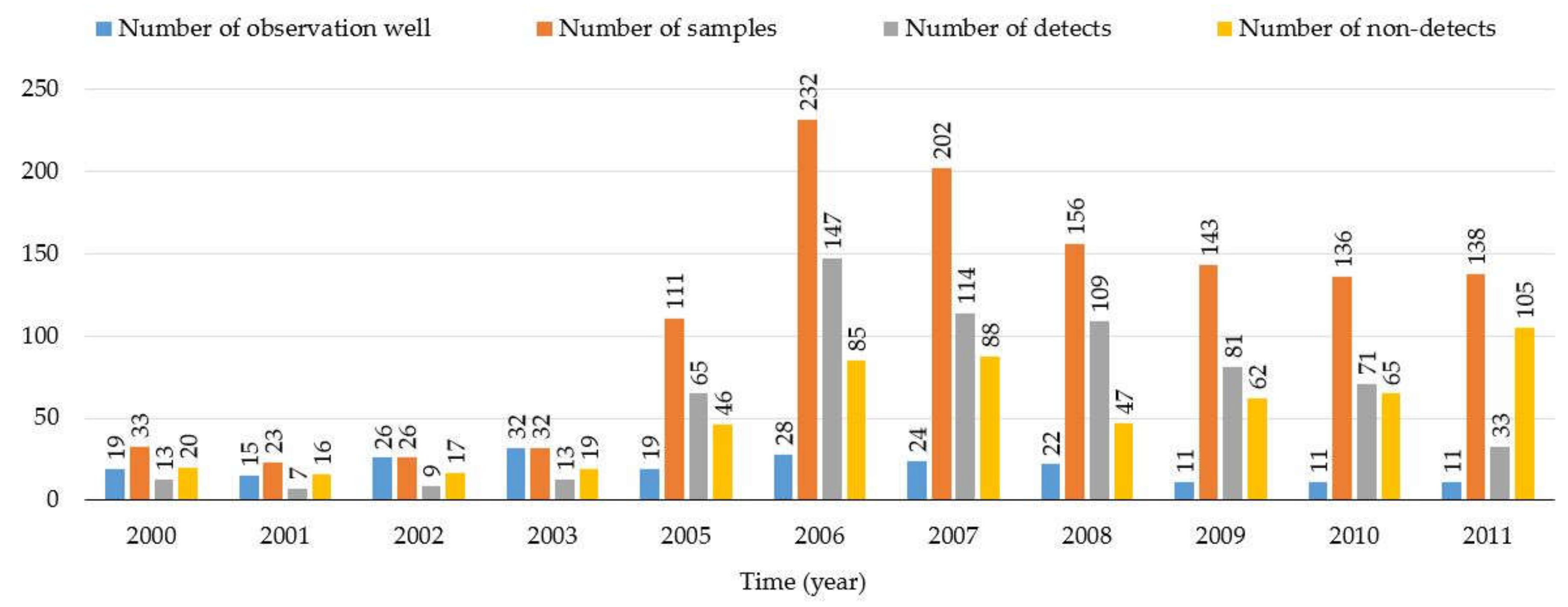
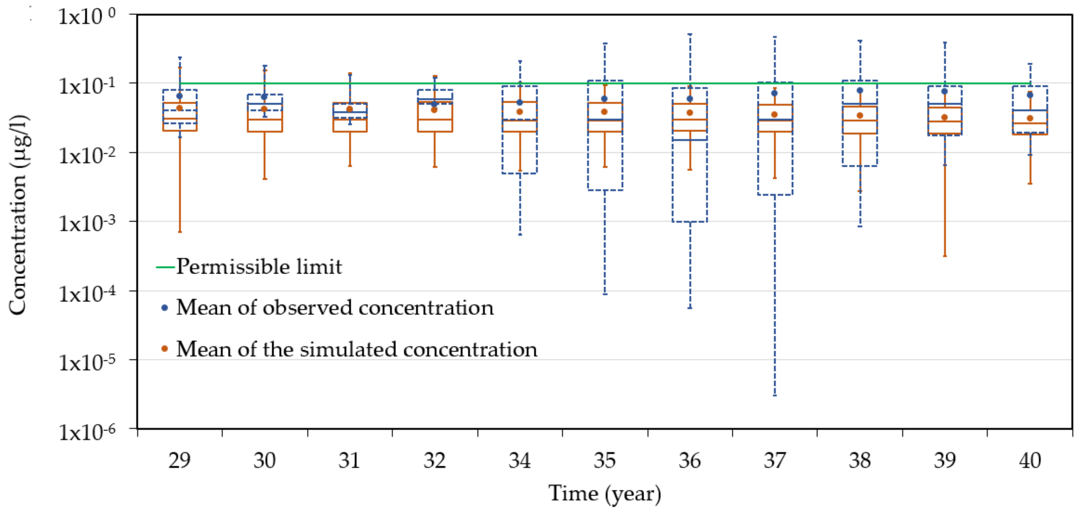
3.3. Comparison of Observed and Model-Simulated Average Annual Atrazine Concentrations

Vonberg et al. [20] conducted a detailed study of atrazine concentrations in groundwater of the Zwischenscholle aquifer based on observations in monitoring wells. This study showed that several modifications and changes were adopted during the monitoring program. The number and location of monitoring wells, the number of samples collected, and the number of detects and non-detects in the samples collected were different over time. Observation wells with small or no atrazine concentrations were excluded, and some wells with higher concentrations were added during the monitoring program [20]. Figure 15 shows the total number of wells, the number of samples, and the number of detects and non-detects. This data collected for the study by Vonberg et al. [20] was not sufficient to make a conclusive statement about the change in the atrazine concentration in the aquifer. In addition to this, there is only limited knowledge about the actual location, quantity, and time of the atrazine application in the study area. Therefore, a direct comparison between simulated and observed solute concentrations with respect to the location and time of atrazine applications is not possible. Nonetheless, in order to validate the performance of the model, the average annual atrazine concentration in groundwater simulated by the model is compared here with the average annual atrazine concentration obtained from field measurements. The years from 2000 to 2011 correspond to 29th to 40th year in the simulation study. Observation data is not available for the year 2004 (33rd year in the simulation study).

Figure 16 shows boxplots of the annual atrazine concentration observed in monitoring wells, and model-simulated concentrations along with the mean of observed and simulated concentrations between years 29 and 40 (except for the year 33). The average annual atrazine concentration in the aquifer obtained using MODFLOW with the HYDRUS-1D package and MT3DMS over the entire simulation period was found to be below the threshold level suggested by the European Council Directive 98/83/EC “The quality of water intended for human consumption” (1998) [29] (0.1 μg/L). The means of observed and simulated atrazine concentrations were found to be comparable. The mean atrazine concentration in observation wells is closer to the threshold level than the model-simulated values, which is mainly because of the addition of monitoring wells, which showed higher concentrations, and the exclusion of wells, which showed smaller concentrations in the monitoring program as explained earlier in this section. Similar observations were made in several other studies on the fate of atrazine in the Zwischenscholle aquifer and other parts of Germany, showing concentrations close to the threshold limit [21,24,69] even after several years of atrazine ban in the country.

The boxplots of the observed and simulated atrazine concentrations show that simulated ranges are narrower than those observed, likely because of the mixing of local concentrations due to dispersion and numerical averaging over 200 × 200 m grid cells. The groundwater sampling is restricted to the volume of groundwater that is sampled in a single observation well. In groundwater transport models, a macroscopic dispersion coefficient is used to represent the effect of aquifer heterogeneity on the solute plume spreading. However, advection dominated spreading can be much larger than mixing and dilution controlled by local-scale dispersion. Therefore, local measured concentrations may vary much more than simulated concentrations because local transport heterogeneities are not averaged out by local measurements.

4. Concluding Remarks

The atrazine contamination in the Zwischenscholle aquifer was analyzed in this study using MODFLOW with the HYDRUS-1D package and MT3DMS. The simulated and observed water table levels and atrazine concentrations were comparable. Model simulations indicate that the variability in the atrazine application rate and the volume of water entering and leaving the aquifer through various sinks and sources led to the variations in the amount of atrazine and its spread in the aquifer. The impact of these different fluxes and their variability was assessed using the model. The long-term analysis of the impact of the atrazine application in the study area shows that the atrazine is persisting in groundwater even after 20 years of its ban. Similar observations were made by Vonberg et al. [20,21] after the detailed investigation of observed atrazine concentrations in the observation wells in the study area.

Though the simulation model can, in general, model the effects of aquifer heterogeneity and various other factors that affect the movement of atrazine in the aquifer, the model was not able to accurately explain the heterogeneous distribution of atrazine concentrations in the aquifer (observed in the monitoring study of Vonberg et al. [20,21]) because of the limited knowledge about the exact quantity and location of atrazine applications in the study area.

The model could not resolve the small-scale transport variability in the aquifer since concentrations and flow velocities were averaged over 200 × 200 m grid cells. Concentrations monitored in groundwater monitoring wells are influenced by these small-scale heterogeneities. The variation of concentrations observed in different monitoring wells can, therefore, be larger than the spatial variation of simulated concentrations. Simulations explained that an observed increase in atrazine concentrations in individual observation wells after the stop of atrazine applications were the result of transport processes in the aquifer, in combination with spatial variations of atrazine leaching from the soil to the aquifer that generated spatial heterogeneity of atrazine concentrations in the groundwater. Presented simulations demonstrate the great modeling capabilities of the coupled modeling system involving MODFLOW with the HYDRUS-1D package and MT3DMS.

References

1. Huang, F.; Li, Z.; Zhang, C.; Habumugisha, T.; Liu, F.; Luo, X. Pesticides in the typical agricultural groundwater in Songnen plain, northeast China: Occurrence, spatial distribution and health risks. Environ. Geochem. Health 2019, 41, 2681–2695. [Google Scholar] [CrossRef] [PubMed]
2. Ali, N.; Khan, S.; Ur Rahman, I.; Muhammad, S. Human health risk assessment through consumption of organophosphate pesticide-contaminated water of Peshawar basin, Pakistan. Expo. Health 2018, 10, 259–272. [Google Scholar] [CrossRef]
3. Gupta, S.D.; Mukherjee, A.; Bhattacharya, J.; Bhattacharya, A. An overview of agricultural pollutants and organic contaminants in groundwater of India. In Groundwater of South Asia; Springer: Singapore, 2018; pp. 247–255. [Google Scholar]
4. El Alfy, M.; Faraj, T. Spatial distribution and health risk assessment for groundwater contamination from intensive pesticide use in arid areas. Environ. Geochem. Health 2017, 39, 231–253. [Google Scholar] [CrossRef] [PubMed]
5. Chaza, C.; Sopheak, N.; Mariam, H.; David, D.; Baghdad, O.; Moomen, B. Assessment of pesticide contamination in Akkar groundwater, northern Lebanon. Environ. Sci. Pollut. Res. 2018, 25, 14302–14312. [Google Scholar] [CrossRef]
6. Pan, H.; Lei, H.; He, X.; Xi, B.; Han, Y.; Xu, Q. Levels and distributions of organochlorine pesticides in the soil–groundwater system of vegetable planting area in Tianjin City, Northern China. Environ. Geochem. Health 2017, 39, 417–429. [Google Scholar] [CrossRef]
7. Sieczka, A.; Bujakowski, F.; Falkowski, T.; Koda, E. Morphogenesis of a floodplain as a criterion for assessing the susceptibility to water pollution in an agriculturally rich valley of a lowland river. Water 2018, 10, 399. [Google Scholar] [CrossRef] [Green Version]
8. Segerson, K. Liability for groundwater contamination from pesticides. Econ. Water Qual. 2018, 19, 227–243. [Google Scholar]
9. Srivastav, A.L. Chemical fertilizers and pesticides: Role in groundwater contamination. In Agrochemicals Detection, Treatment and Remediation; Elsevier: Amsterdam, The Netherlands, 2020; pp. 143–159. [Google Scholar]
10. Worrall, F.; Besien, T. The vulnerability of groundwater to pesticide contamination estimated directly from observations of presence or absence in wells. J. Hydrol. 2005, 303, 92–107. [Google Scholar] [CrossRef]
11. Thapinta, A.; Hudak, P.F. Use of geographic information systems for assessing groundwater pollution potential by pesticides in Central Thailand. Environ. Int. 2003, 29, 87–93. [Google Scholar] [CrossRef] [Green Version]
12. Papadopoulou-Mourkidou, E.; Karpouzas, D.G.; Patsias, J.; Kotopoulou, A.; Milothridou, A.; Kintzikoglou, K.; Vlachou, P. The potential of pesticides to contaminate the groundwater resources of the Axios river basin in Macedonia, Northern Greece. Part I. Monitoring study in the north part of the basin. Sci. Total Environ. 2004, 321, 127–146. [Google Scholar] [CrossRef]
13. Leterme, B.; Vanclooster, M.; Rounsevell, M.D.A.; Bogaert, P. Discriminating between point and non-point sources of atrazine contamination of a sandy aquifer. Sci. Total Environ. 2006, 362, 124–142. [Google Scholar] [CrossRef] [PubMed]
14. Tiktak, A.; De Nie, D.S.; Garcet, J.D.P.; Jones, A.O.; Vanclooster, M. Assessment of the pesticide leaching risk at the Pan-European level. The EuroPEARL approach. J. Hydrol. 2004, 289, 222–238. [Google Scholar] [CrossRef]
15. Loague, K.; Soutter, L.A. Desperately seeking a cause for hotspots in regional-scale groundwater plumes resulting from non-point source pesticide applications. Vadose Zone J. 2006, 5, 204–221. [Google Scholar] [CrossRef]
16. Franke, H.-J.; Teutsch, G. Stochastic simulation of the regional pesticide transport including the unsaturated and the saturated zone. Ecol. Model. 1994, 75, 529–539. [Google Scholar] [CrossRef]
17. Kupfersberger, H.; Klammler, G.; Schumann, A.; Brückner, L.; Kah, M. Modeling subsurface fate of s-metolachlor and metolachlor ethane sulfonic acid in the Westliches Leibnitzer Feld aquifer. Vadose Zone J. 2018, 17, 170030. [Google Scholar] [CrossRef] [Green Version]
18. Honeycutt, R. Mechanisms of Pesticide Movement into Ground Water; CRC Press: Boca Raton, FL, USA, 2018; ISBN 1351082795. [Google Scholar]
19. Jones, R.L. Modeling the degradation and movement of agricultural chemicals in ground water. In Mechanisms of Pesticide Movement into Ground Water; CRC Press: Boca Raton, FL, USA, 2018. [Google Scholar]
20. Vonberg, D.; Vanderborght, J.; Cremer, N.; Pütz, T.; Herbst, M.; Vereecken, H. 20 years of long-term atrazine monitoring in a shallow aquifer in western Germany. Water Res. 2014, 50, 294–306. [Google Scholar] [CrossRef]
21. Vonberg, D.; Hofmann, D.; Vanderborght, J.; Lelickens, A.; Köppchen, S.; Pütz, T.; Burauel, P.; Vereecken, H. Atrazine soil core residue analysis from an agricultural field 21 years after its ban. J. Environ. Qual. 2014, 43, 1450. [Google Scholar] [CrossRef]
22. Farlin, J.; Drouet, L.; Gallé, T.; Pittois, D.; Bayerle, M.; Braun, C.; Maloszewski, P.; Vanderborght, J.; Elsner, M.; Kies, A. Delineating spring recharge areas in a fractured sandstone aquifer (Luxembourg) based on pesticide mass balance. Hydrogeol. J. 2013, 21, 799–812. [Google Scholar] [CrossRef]
23. Gutierrez, A.; Baran, N. Long-term transfer of diffuse pollution at catchment scale: Respective roles of soil, and the unsaturated and saturated zones (Brévilles, France). J. Hydrol. 2009, 369, 381–391. [Google Scholar] [CrossRef]
24. Tappe, W.; Groeneweg, J.; Jantsch, B. Diffuse atrazine pollution in German aquifers. Biodegradation 2002, 13, 3–10. [Google Scholar] [CrossRef]
25. Dunlap, K.; Brown, A. Atrazine Levels in Water, Sediment, and Amphibian Tissue Samples from Selected Ponds in Westernmost Kentucky; Murray State University: Murray, KY, USA, 2018. [Google Scholar]
26. Guzzella, L.; Pozzoni, F.; Giuliano, G. Herbicide contamination of surficial groundwater in Northern Italy. Environ. Pollut. 2006, 142, 344–353. [Google Scholar] [CrossRef] [PubMed]
27. Jayachandran, K.; Steinheimer, T.R.; Somasundaram, L.; Moorman, T.B.; Kanwar, R.S.; Coats, J.R. Occurrence of atrazine and degradates as contaminants of subsurface drainage and shallow groundwater. J. Environ. Qual. 1994, 23, 311–319. [Google Scholar] [CrossRef] [Green Version]
28. Wehtje, G.; Leavitt, J.R.C.; Spalding, R.F.; Mielke, L.N.; Schepers, J.S. Atrazine contamination of groundwater in the Platte Valley of Nebraska from non-point sources. Sci. Total Environ. 1981, 21, 47–51. [Google Scholar] [CrossRef]
29. Regulation, E.U. Council Directive 98/83/EC of 3 November 1998 on the quality of water intended for human consumption. Off. J. Eur. Commun. 1998, 41, 32–54. [Google Scholar]
30. Herbst, M.; Hardelauf, H.; Harms, R.; Vanderborght, J.; Vereecken, H. Pesticide fate at regional scale: Development of an integrated model approach and application. Phys. Chem. Earth Parts A/B/C 2005, 30, 542–549. [Google Scholar] [CrossRef]
31. Mouvet, C.; Baran, N.; Thiery, D.; Gutierrez, A.; Darsy, C.; Dubus, I.G.; Falkiewicz, W.; Ritsema, C.; Dekker, L.; Normand, B. Pesticides in European groundwaters: Detailed study of representative aquifers and simulation of possible evolution scenarios (PEGASE). In Proceedings of the EU Workshop: The Functioning and Management of the Water-Soil-System at River-Basin Scale: Diffuse Polltuion and Point Sources, Orléans, France, 26–28 November 2003; pp. 248–263. [Google Scholar]
32. Suffet, I.H.; Gibs, J.; Coyle, J.A.; Chrobak, R.S.; Yohe, T.L. Applying analytical techniques to solve groundwater contamination problems. J. Am. Water Works Assoc. 1985, 77, 65–72. [Google Scholar] [CrossRef]
33. Walton, W.C. Analytical Groundwater Modeling Flow and Contaminant Migration; Lewis Publishers: Chelsea, MI, USA, 1989. [Google Scholar]
34. Aller, L. DRASTIC: A Standardized System for Evaluating Ground Water Pollution Potential Using Hydrogeologic Settings; Robert, S., Ed.; Kerr Environmental Research Laboratory, Office of Research and Development, US Environmental Protection Agency: Washington, DC, USA, 1985. [Google Scholar]
35. Bartzas, G.; Tinivella, F.; Medini, L.; Zaharaki, D.; Komnitsas, K. Assessment of groundwater contamination risk in an agricultural area in north Italy. Inf. Process. Agric. 2015, 2, 109–129. [Google Scholar] [CrossRef] [Green Version]
36. Djoudi, S.; Boulabiez, F.; Pistre, S.; Houha, B. Assessing Groundwater Vulnerability to Contamination in a Semi-Arid Environment Using DRASTIC and GOD Models, Case of F’kirina Plain, North of Algeria. IOSR J. Environ. Sci., Toxicol. Food Technol. 2019, 13, 39–44. [Google Scholar]
37. Al-Adamat, R.; Al-Shabeeb, A.A.-R. A simplified method for the assessment of groundwater vulnerability to contamination. J. Water Resour. Protect. 2017, 9, 305. [Google Scholar] [CrossRef] [Green Version]
38. Civita, M.; De Maio, M.; Ubertini, L. Valutazione e cartografia automatica della vulnerabilità degli acquiferi all’inquinamento con il sistema parametrico Sintacs R5: A new parametric system for the assessment and automatic mapping of ground water vulnerability to contamination; Pitagora: Bologna, Italy, 2000; ISBN 8837112319. [Google Scholar]
39. Fusco, F.; Allocca, V.; Coda, S.; Cusano, D.; Tufano, R.; De Vita, P. Quantitative assessment of specific vulnerability to nitrate pollution of shallow alluvial aquifers by process-based and empirical approaches. Water 2020, 12, 269. [Google Scholar] [CrossRef] [Green Version]
40. Michalak, A.M.; Shlomi, S. A geostatistical data assimilation approach for estimating groundwater plume distributions from multiple monitoring events. Geophys. Monogr. Am. Geophys. Union 2007, 171, 73. [Google Scholar]
41. McLean, M.I.; Evers, L.; Bowman, A.W.; Bonte, M.; Jones, W.R. Statistical modelling of groundwater contamination monitoring data: A comparison of spatial and spatiotemporal methods. Sci. Total Environ. 2019, 652, 1339–1346. [Google Scholar] [CrossRef] [PubMed]
42. Lappala, E.G.; Healy, R.W.; Weeks, E.P. Documentation of Computer Program VS2D to Solve the Equations of Fluid Flow in Variably Saturated Porous Media; Department of the Interior, US Geological Survey: Reston, VA, USA, 1987; p. 83. [Google Scholar]
43. Zheng, C.; Wang, P.P. MT3DMS: A Modular Three-Dimensional Multispecies Transport Model for Simulation of Advection, Dispersion, and Chemical Reactions of Contaminants in Groundwater Systems; Documentation and User’s Guide; Alabama University: Tuscaloosa, AL, USA, 1999. [Google Scholar]
44. Xu, T.; Sonnenthal, E.; Spycher, N.; Pruess, K. TOUGHREACT: A New Code of the TOUGH Family for Non-Isothermal Multiphase Reactive Geochemical Transport in Variably Saturated Geologic Media; University of California: Berkeley, CA, USA, 2003. [Google Scholar]
45. Healy, R.W. Simulation of Solute Transport Invariably Saturated Porous Media with Supplemental Information on Modifications to the US Geological Survey’s Computer Program VS2D; Department of the Interior, US Geological Survey: Reston, VA, USA, 1990; p. 90. [Google Scholar]
46. Šimůnek, J.; van Genuchten, M.T.; Šejna, M. The HYDRUS-1D software package for simulating the one-dimensional movement of water, heat, and multiple solutes in variably-saturated media. Univ. Calif. Riverside Res. Rep. 2005, 3, 1–240. [Google Scholar]
47. Šimůnek, J.; Bradford, S.A. Vadose zone modeling: Introduction and importance. Vadose Zone J. 2008, 7, 581–586. [Google Scholar] [CrossRef]
48. Refsgaard, J.; Storm, B. Computer models of watershed hydrology, MIKE SHE. Water Resour. Publ. 1995, 809–846. [Google Scholar]
49. Twarakavi, N.K.C.; Simunek, J.; Seo, S. Evaluating interactions between groundwater and vadose zone using the HYDRUS-based flow package for MODFLOW. Vadose Zone J. 2008, 7, 757–768. [Google Scholar] [CrossRef] [Green Version]
50. Brunner, P.; Simmons, C.T. HydroGeoSphere: A fully integrated, physically based hydrological model. Groundwater 2012, 50, 170–176. [Google Scholar] [CrossRef] [Green Version]
51. Kalbacher, T.; Delfs, J.O.; Shao, H.; Wang, W.; Walther, M.; Samaniego, L.; Schneider, C.; Kumar, R.; Musolff, A.; Centler, F.; et al. The IWAS-ToolBox: Software coupling for an integrated water resources management. Environ. Earth Sci. 2012, 65, 1367–1380. [Google Scholar] [CrossRef]
52. Morway, E.D.; Niswonger, R.G.; Langevin, C.D.; Bailey, R.T.; Healy, R.W. Modeling variably saturated subsurface solute transport with MODFLOW-UZF and MT3DMS. GroundWater 2013, 51, 237–251. [Google Scholar] [CrossRef]
53. Beegum, S.; Šimůnek, J.; Szymkiewicz, A.; Sudheer, K.P.; Nambi, I.M. Implementation of solute transport in the vadose zone into the “HYDRUS Package for MODFLOW. ” Groundwater 2019, 57, 392–408. [Google Scholar] [CrossRef] [Green Version]
54. Beegum, S.; Šimůnek, J.; Szymkiewicz, A.; Sudheer, K.P.; Nambi, I.M. Updating the coupling algorithm between HYDRUS and MODFLOW in the HYDRUS Package for MODFLOW. Vadose Zone J. 2018, 17, 180034. [Google Scholar] [CrossRef] [Green Version]
55. Mouvet, C.; Albrechtsen, H.J.; Baran, N.; Chen, T.; Clausen, L.; Darsy, C. PEGASE. Pesticides in European Groundwaters: Detailed Study of Representative Aquifers and Simulation of possible Evolution Scenarios; Final Report of the European Project; UW Umweltwirtschaft GmbH: Stuttgart, Germany, 2004. [Google Scholar]
56. Lahmeyer Site appraisal of geology, hydrogeology and soil mechanics (Standortgutachten Geologie, Hydrogeologie und Bodenmechanik). Unpublished work. 1984.
57. Seo, H.S.; Šimůnek, J.; Poeter, E.P. Documentation of the HYDRUS Package for MODFLOW -2000, the US Geological Survey Modular Ground Water Model. GWMI 2007-01, IGWMC-International Ground Water Modeling Center; Colorado School of Mines: Golden, CO, USA, 2007; p. 96. [Google Scholar]
58. Harbaugh, A.W.; Banta, E.R.; Hill, M.C.; Mcdonald, M.G. MODFLOW-2000, the US Geological Survey modular ground-water model: User guide to modularization concepts and the ground-water flow process. USA Geol. Surv. 2000, 1–92. [Google Scholar]
59. Šimůnek, J.; van Genuchten, M.T.; Šejna, M. Recent developments and applications of the HYDRUS computer software packages. Vadose Zone J. 2016, 15. [Google Scholar] [CrossRef] [Green Version]
60. Šimůnek, J.; van Genuchten, M.T. Modeling nonequilibrium flow and transport processes using HYDRUS. Vadose Zone J. 2008, 7, 782–797. [Google Scholar] [CrossRef] [Green Version]
61. Bogena, H. MOSYRUR: Water Balance Analysis in the Rur Basin; Heye Bogena, Forschungszentrum, Zentralbibliothek: Julich, Germany, 2005. [Google Scholar]
62. van Genuchten, M.T. A closed-form equation for predicting the hydraulic conductivity of unsaturated soils. Soil Sci. Soc. Am. J. 1980, 44, 892–898. [Google Scholar] [CrossRef] [Green Version]
63. Spitters, C.J.T.; Van Keulen, H.; Van Kraalingen, D.W.G. A simple and universal crop growth simulator: SUCROS87. In Simulation and Systems Management in Crop Protection; Rabbinge, R., Ward, S.A., van Laar, H.H., Eds.; Pudoc: Wageningen, The Netherlands, 1989; pp. 147–181. ISBN 9022008991. [Google Scholar]
64. Doorenbos, J.; Pruitt, W.O. Crop Water Requirements. FAO Irrigation and Drainage Paper 24; Land and Water Development Division; FAO: Rome, Italy, 1977; p. 144. [Google Scholar]
65. Feddes, R.A.; Kowalik, P.J.; Zaradny, H. Simulation of Field Water Use and Crop Yield; John Wiley and Sons: New York, NY, USA, 1978. [Google Scholar]
66. Rakowski, P.; Knowling, M.J. Heretaunga Aquifer Groundwater Model: Development Report; HBRC Report No RM18-14-4997; Hawke’s Bay Regional Council: Napier, New Zealand, 2018. [Google Scholar]
67. Nachabe, M.H. Analytical expressions for transient specific yield and shallow water table drainage. Water Resour. Res. 2002, 38, 11. [Google Scholar] [CrossRef] [Green Version]
68. Said, A.; Nachabe, M.; Ross, M.; Vomacka, J. Methodology for estimating specific yield in shallow water environment using continuous soil moisture data. J. Irrig. Drain. Eng. 2005, 131, 533–538. [Google Scholar] [CrossRef]
69. Jablonowski, N.D.; Köppchen, S.; Hofmann, D.; Schäffer, A.; Burauel, P. Persistence of 14C-labeled atrazine and its residues in a field lysimeter soil after 22 years. Environ. Pollut. 2009, 157, 2126–2131. [Google Scholar] [CrossRef] [Green Version]
Figure 1. Study area with geological faults and observation wells.
Water 12 01019 g001
Figure 2. Cross-sections A-A’ and B-B’ of the aquifer presented in Figure 1.
Water 12 01019 g002
Figure 3. The daily precipitation and potential reference evapotranspiration data for the study area from 1984 to 1993.
Water 12 01019 g003
Figure 4. Land use from 1984 to 1993.
Water 12 01019 g004
Figure 5. The total mass of applied atrazine (a) and the area of the atrazine application in the study area (b) from 1984 to 1993.
Water 12 01019 g005
Figure 6. The initial water table elevation, MODFLOW grids, boundary condition, the general groundwater flow direction (the blue arrow), and the thickness of the aquifer at four boundary points.
Water 12 01019 g006
Figure 7. Comparison of water table fluctuations in observation wells (observed) and those simulated using MODFLOW with the HYDRUS-1D package (simulated).
Water 12 01019 g007
Figure 8. Average annual atrazine concentrations in the aquifer simulated using MODFLOW with the HYDRUS-1D package and MT3DMS.
Water 12 01019 g008
Figure 9. Total net recharge and the net recharge rate between the unsaturated and saturated soil zones in each year.
Water 12 01019 g009
Figure 10. Volumes of water entering and leaving through sides of the domain (a), and water fluxes entering and leaving the aquifer through sides of the domain (b), (Side 1_in to Side 4_in represent flow entering through particular lateral sides, and Side 1_out to Side 4_out represent flow leaving through particular lateral sides).
Water 12 01019 g010
Figure 11. The total mass of atrazine that is entering the aquifer through various sources and leaving the aquifer through various sinks (a), and the total mass of atrazine that is entering the aquifer through lateral inflow and recharge (b).
Water 12 01019 g011
Figure 12. The amount of atrazine entering and leaving the aquifer through four lateral sides (Side 4_in represents atrazine volumes entering through Side 4, Side 1_out to Side 4_out represent atrazine leaving through corresponding lateral sides, and Total Sides_out represents the amount of solute leaving though all lateral sides).
Water 12 01019 g012
Figure 13. The spatial pattern of the atrazine concentration (μg/L) in the aquifer from year 1 to year 40 (a logarithmic color scale).
Water 12 01019 g013
Figure 14. Atrazine concentrations in six observation wells after 20 years of atrazine application (a), and the locations of the observation wells (b).
Water 12 01019 g014
Figure 15. The number of observation wells, samples collected, samples with detects and non-detects from the monitoring program in the Zwischenscholle aquifer [20,21].
Water 12 01019 g015
Figure 16. Boxplots of the annual atrazine concentrations observed in monitoring wells (represented in blue color) and simulated (represented in brown color), along with the arithmetic mean of observed and simulated atrazine concentrations (a logarithmic scale).
Water 12 01019 g016