Model Analysis and System Parameters Investigation for Transient Wave in a Pump–Pipe–Valve System


1
B&K-ZJUT Joint Sound and Vibration Lab, Department of Mechanical Engineering, Zhejiang University of Technology, Hangzhou 310014, China
2
Department of Engineering Mechanics, Zhejiang University, Hangzhou 310027, China
3
Department of Ocean Engineering, Zhejiang University, Zhoushan 316021, China
4
Faculty of Mechanical Engineering & Automation, Zhejiang Sci-Tech University, Hangzhou 310018, China
*
Author to whom correspondence should be addressed.
Water 2020, 12(4), 1014; https://doi.org/10.3390/w12041014
Submission received: 14 March 2020
/
Revised: 29 March 2020
/
Accepted: 31 March 2020
/
Published: 2 April 2020
(This article belongs to the Section Hydraulics and Hydrodynamics)
Abstract
:The frequency responses of the transient wave propagating in a pump–pipe–valve system are studied with the system transfer matrix analysis (STMA) method. Being different to that in the reservoir–pipe–valve system, the transient wave is used as a long-distance communication technology in the pump–pipe–valve system, and very few works have been done on the model analysis and strategies to control the behavior of the oscillation signal of the pipe pressure. The theoretic solutions are studied with three internal friction models: frictionless, steady friction, and unsteady friction. The dimensionless parameter of the valve signal intensity (VSI) is proposed, and it is found to be a key factor affecting the quality of the wave propagation in the pipe. A larger pressure oscillation at the upstream side results when the VSI is smaller than one, whereas a more uniform amplitude for the resonances and anti-resonances is obtained when VSI approaches one. Some feasible suggestions are provided to obtain high quality wave signals.
1. Introduction
The pump–pipe–valve system, composed of a pump at the inlet, a transporting pipeline, and an ending valve, is always used for long-distance transportation of fluid. The fluid discharge in this system can be assumed to be constantly served by a reciprocating pump, i.e., the fluid is pumped into the pipeline with an invariable velocity even though the pressure at the pipe inlet is varying. Owing to the particular setup of the boundary condition, characteristics of the transient wave propagation in the pump–pipe–valve system would be different than those in the reservoir–pipe–valve system. However, the pump–pipe–valve system has rarely been investigated in the past. In order to provide reasonable frequency domain selections for transient wave communication in long-distance oil/water pipelines, it is valuable to study the frequency response of periodic transient waves in the pump–pipe–valve system.
The frequency response describes how the system affects each individual frequency component of the input transient signal, and it was first proposed for the measurements in the human vocal tract by Schroeder [1] and Mermelstein [2]. The acoustic impedance of the system is represented by an approximate function of the dimensions of the internal structures and can be measured by the comparison of the source and the reflection at a frequency range. These techniques aim to detect extended blockages in the human vocal tract by observing the measured shifts of the resonant frequencies within gas transmission in the pipeline system. Then, Qunli and Fergus [3,4] improved the method with an approximation of the resonance frequency shifts, which was determined from a single maximum length sequence (MLS) measurement in the partially blocked duct, since the MLS signals have inherently high noise immunity and provide a large enough signal-to-noise ratio. Later on, the anti-resonance frequencies were considered by De Salis and Oldham [5,6] to obtain a simpler blockage reconstruction function with a single pressure response measurement. Çelik et al. [7] introduced numerical simulations on a stepped-tube model to evaluate the influences of the internal shape of the nasal cavity on acoustic rhinometry (AR) measurements. Pulse reflectometry is another type of frequency response that is used as a non-intrusive measuring technique to obtain internal measurements of tubular objects [8,9]. Sharp and Campbell [10,11] extended the method to leakage detection, such as an internal bore, in pipes with the internal reflection of the impulse, and to measure the internal structure for wind instruments such as trumpet and cornet. Both technologies are effective methods to find out the variation of the cross-sections in pipes by implying the reflection measurement from a signal of acoustic impulse, but the demerit is useless on the more-than-one discrete changes in the pipe. Besides, previous research concentrated on transient waves in airflow, e.g., musical instruments, but rarely in hydraulic systems, i.e., in liquid flow.
In the past three decades, the unsteady transient wave caused by a sudden change is simulated by the method of characteristics (MOC) for time-domain problems, while the steady periodic wave propagation is obtained by the system transfer matrix analysis (STMA) in the frequency domain. In hydraulic systems, the frequency response analysis was also studied using STMA, with periodic transient signals for the steady-oscillatory flows [12]. In detail, the field matrix is introduced to represent the transfer process between the input and the output, assuming that the pipeline is a linear hydraulic system. Thus, the pipelines act as “frequency filters”, reinforcing and transmitting input signals at particular frequencies, i.e., resonant frequencies, and effectively absorbing and attenuating signals at other frequencies, i.e., anti-resonant frequencies [13]. The method is widely used to detect the leakage and blockage in water supply pipe systems and oil pipelines. The transfer matrix equations were proposed to detect the leakage in a single pipe with the relative size of resonance peaks at certain odd harmonic frequencies [13,14,15,16,17]. Verde [18] reconstructed two leaks in a pipeline, while Guillen [19] provided a model to obtain system frequency response with two observers at the inlet and outlet, respectively. On the other hand, the detection of the blockage in the pipeline was also developed. Mohapatra et al. [20,21] and Sattar [22] used the pattern and the numbers of peaks at the odd-harmonics frequency for detecting blockage location and the mean peak pressure fluctuations to determine the size of a single blockage. Later, the detection for the discrete blockages [23] and the extended blockage [24,25] was developed with improved approaches of the system frequency responses. Meniconi [26] experimentally investigated the frequency domain transient response for the detection of partial blockage compared with the time domain analysis. Duan and Lee [27,28] recently proposed a new model to detect the branch pipe in pipe systems and studied the influence of irregularity of blockages and roughness of pipe on the accuracy of the blockage detection by the frequency response. The resonances shift in the blockage detection system with the STMA method was considered as Bragg resonance effects in a reservoir–pipe–valve (RPV) [29].
Recently, in order to improve the applicability and accuracy of the numerical model, a modified 2D model for the pipe section [30] and a virtual valve method for large size valve perturbation [31] were proposed, and the former indicated the radial pressure wave should be considered with viscous fluid, while the latter made a correction for the biases of system response at high frequency. The linearized error of the 1D water hammer model was analyzed and it was found that perturbation of the steady state condition has a positive correlation with the resultant linearization error [32]. Later, a sensitivity investigation was performed and it was found that the model was more sensitive to the wave speed and data measurement than valve operation and initial hydraulic condition [33]. The frequency response was also applied to inversely identify the viscoelastic parameters of plastic pipe through times of measurement with different flux and operation conditions [34]. Despite the hydraulic system, the pulsation attenuation characteristics of the expansion chamber structure are also studied by the system impedance analysis [35], since the expansion chamber is a popular section in pulsation attenuation devices. It is found that the attenuance is only effective at certain frequencies, which are dependent on the dimensions of the chamber.
In a sum, the system frequency response of a pipeline is mainly used to measure the unknown internal structure, the diameter-varied chamber, the leakage, and the blockage, via the variation of the peak amplitude and frequency shift of the resonance and anti-resonance caused by the variation of the characteristic impedance of the pipeline. In this paper, the boundary conditions of the pump–pipe–valve system are different from those in the reservoir–pipe–valve system, and the latter is the model widely applied in previous work. However, the boundary conditions could greatly affect the resonant and anti-resonant behavior of the system; thorough investigations are demanded. The STMA method is used in this paper to study the system frequency response, and the current investigation aims to avoid the attenuation of the transient wave signals at a certain frequency or a range. The characteristics of the frequency response are obtained, as well as the influences from parameters of the system.
2. Pump–Pipe–Valve System
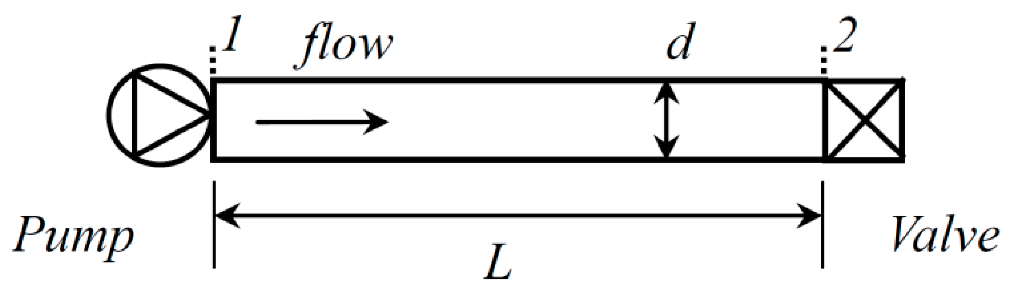
In the pump–pipe–valve system, the fluid flows from the input pump into the pipeline and goes out to the atmosphere through the ending valve. The periodic transient waves are generated via the oscillation of the cross-section of the ending valve. The diagram of the pump–pipe–valve system is shown in Figure 1, where the dimension of the pipeline is defined by the length and diameter of a single pipe. Being different from the reservoir–pipe–valve system, a reciprocating pump serves as the inlet providing a constant discharge into the pipeline. In particular, the displacement of rocker in the pump does not change with the pressure in the pipe, and, therefore, it keeps an invariable flux during the delivery stroke. Thus, the input discharge from the pump can be considered as a constant during the propagation of the transient wave in the pipeline.
3. System Frequency Response
The system frequency response describes the system behavior at the frequency domain, and it is investigated by calculating the amplitudes and phases of the transient wave in the pipeline system. Analyses and numerical simulations are implemented for a single pipeline with both frictionless or and frictional models, and parameters of pipeline structure and fluid are taken into account as the major factors. The amplitudes and frequencies of the resonances and anti-resonances are mainly investigated.
3.1. STMA Model
The flow is pumped into the pipeline while the periodic transient waves are generated by the ending valve at the outlet. The transfer function of the transient wave between the two nodes of the single pipe can be expressed by the STMA [12]
Here, and are the amplitudes of the discharge flux and the pressure fluctuations at the angle frequency , the superscripts represent the left hand () and the right hand () values at certain nodes, which are noted as number 1 and 2 in the Figure 1, the gravity coefficient, the area of cross-section, the transient wave speed in the pipe, the internal diameter, the Darcy-Weisbach friction factor. and are the mean values of pressure head and discharge. The term represents the characteristic impedance of pipe, while is the effect of friction. Here, a frictionless model is represented by , whereas a friction model is represented by . Consequently, the propagation of the transient wave in the pipeline can be represented by a transfer matrix as
When the effects of friction are ignored (), the transfer matrix can be simplified to be
A similar transfer matrix can be derived for the sinusoidal oscillating valve at the outlet of the pipeline. Since the outside of the ending valve is open in the air, the discharge of the ending valve can be calculated by , where is the coefficient of discharge, is the area of valve opening, is the steady-state head loss across the valve. Assuming the linear behavior of the discharge through the valve, the transfer function between the two sides of the node is represented by [12]
with the amplitude of the valve motion, the mean value of the valve opening. Consequently, by substituting Equation (2) into Equation (4), the system transfer matrix of the entire pipeline is obtained as
with matrix elements , . Here, the amplitude is defined as the hydraulic impedance of the outlet valve, and is the magnitude of the pressure oscillation caused by the ending valve.
After adding certain boundary conditions at two ends, the computational model of the transient wave propagation is complete. Since the reciprocating pump can provide a constant flow discharge at the upstream side, the inlet boundary condition is set to be , whereas a constant pressure head is obtained at the outlet, . Thus, two unknown quantities can be solved with two equations. The pressure fluctuations at the upstream and downstream sides of the pipeline can be respectively obtained as
As we know, the maximum magnitude of the pressure fluctuation appears at the resonances of the pipeline system while the minimum comes at the anti-resonances. Similarly, resonances of the reservoir–pipe–valve system have been studied in detail in the past [13,17,19,22,24,26], to depress the damages from the steep rise of pressure head or to detect leakages and blockages in the pipeline system. However, little work takes care of the influence of the parameters of pipeline structure and fluid on the behavior of resonance and anti-resonance.
In order to account the magnitude ratio of the hydraulic impedance of the outlet valve over the characteristic impedance of the pipeline, the dimensionless parameter “valve signal intensity (VSI)” is proposed here and it is defined as
It is found that resonances and anti-resonances of the pressure fluctuations at the upstream side are significantly related to the VSI condition. In detail:
- (1)
- If ,
- (2)
- If ,
- (3)
- If ,
On the contrary, the resonances and anti-resonances at the downstream side are not related to the VSI condition, and they are represented as
It is noted that the upstream pressure fluctuation at the VSI condition is much larger than those at the VSI conditions and since the minimum amplitude at the VSI condition equals the maximums at the other two conditions, which provides an effective method to adjust the amplitude of pressure fluctuation in the pipeline. Furthermore, the VSI condition provides the same amplitude for all the frequency response, which means no attenuation for the signal communication in the pipeline. Thus, the variation of the upstream resonances with the VSI conditions is a valuable clue to choosing the frequency domain to obtain the expected pressure fluctuation at both of the sides in the pipeline.
The frequency interval between two adjacent resonances reads
3.2. Frictionless Model
The numerical simulation is first performed on a single pipe system with the frictionless model to verify the analytical solutions. The dimensions of the pipeline are defined with the length and the diameter , while the wave speed in the pipe is , the amplitude ratio of the valve motion is , the steady-state flow is . According to Equation (7), the head loss across the valve, , can be calculated when the VSI condition is defined. Furthermore, the mean pressure head is invariable along the pipeline and equals to the head loss when the frictionless model is applied; . The frequency range is represented by a dimensionless parameter: , with in numerical results.
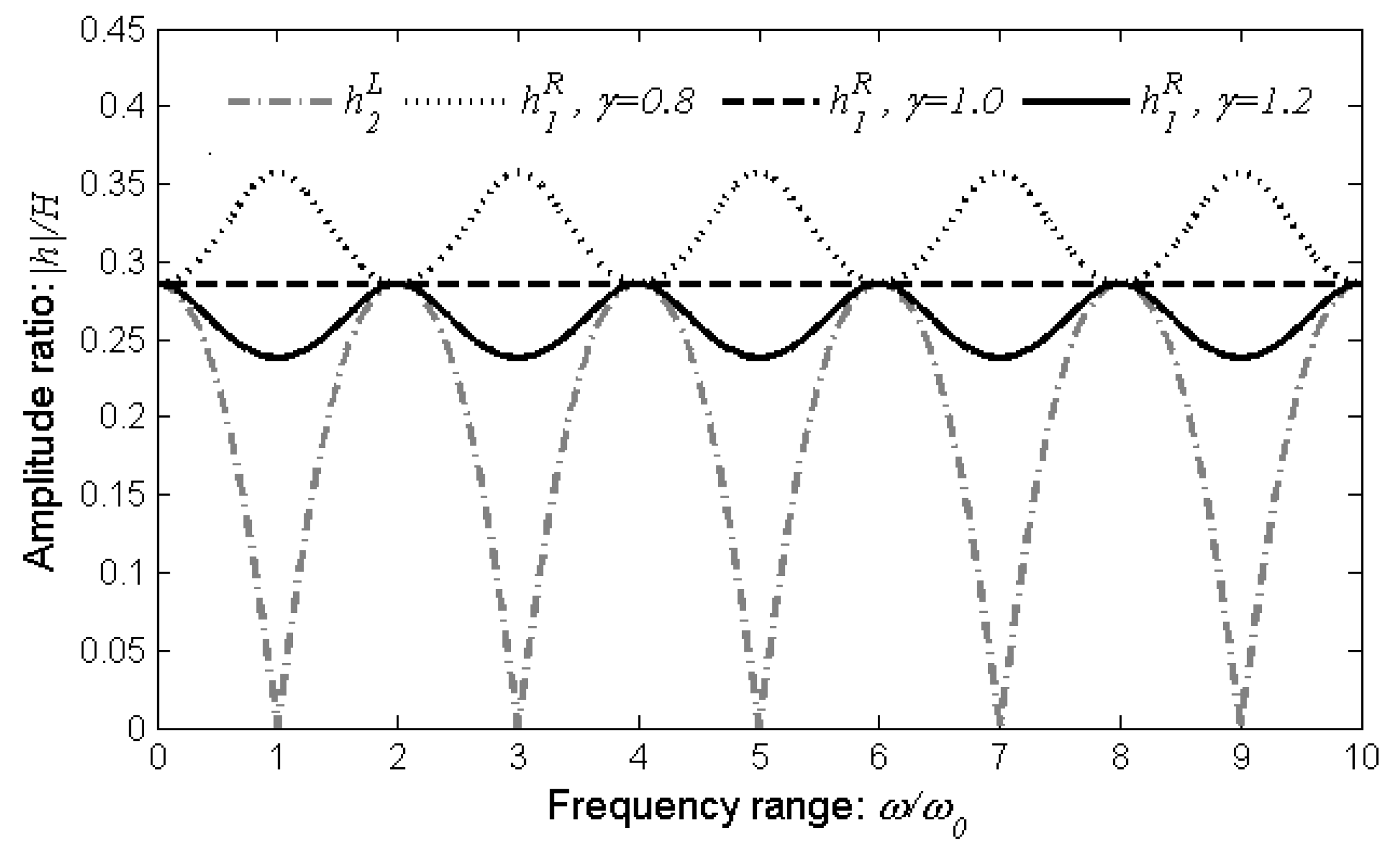
Figure 2 shows the frequency response of the pipeline under three VSI conditions. It is found that the downstream pressure fluctuations on resonances and anti-resonances are independent of the frequency, which coincides with Equations (13) and (14). The behavior of resonances and anti-resonances at the upstream side is strongly dependent on the VSI conditions, as indicated from the results, which is the same as the prediction. The resonances at lower VSI () locate the same frequencies with the anti-resonances frequencies at higher VSI (), and the amplitude of pressure fluctuations at lower VSI condition is larger than that at higher VSI condition regardless of the frequency.
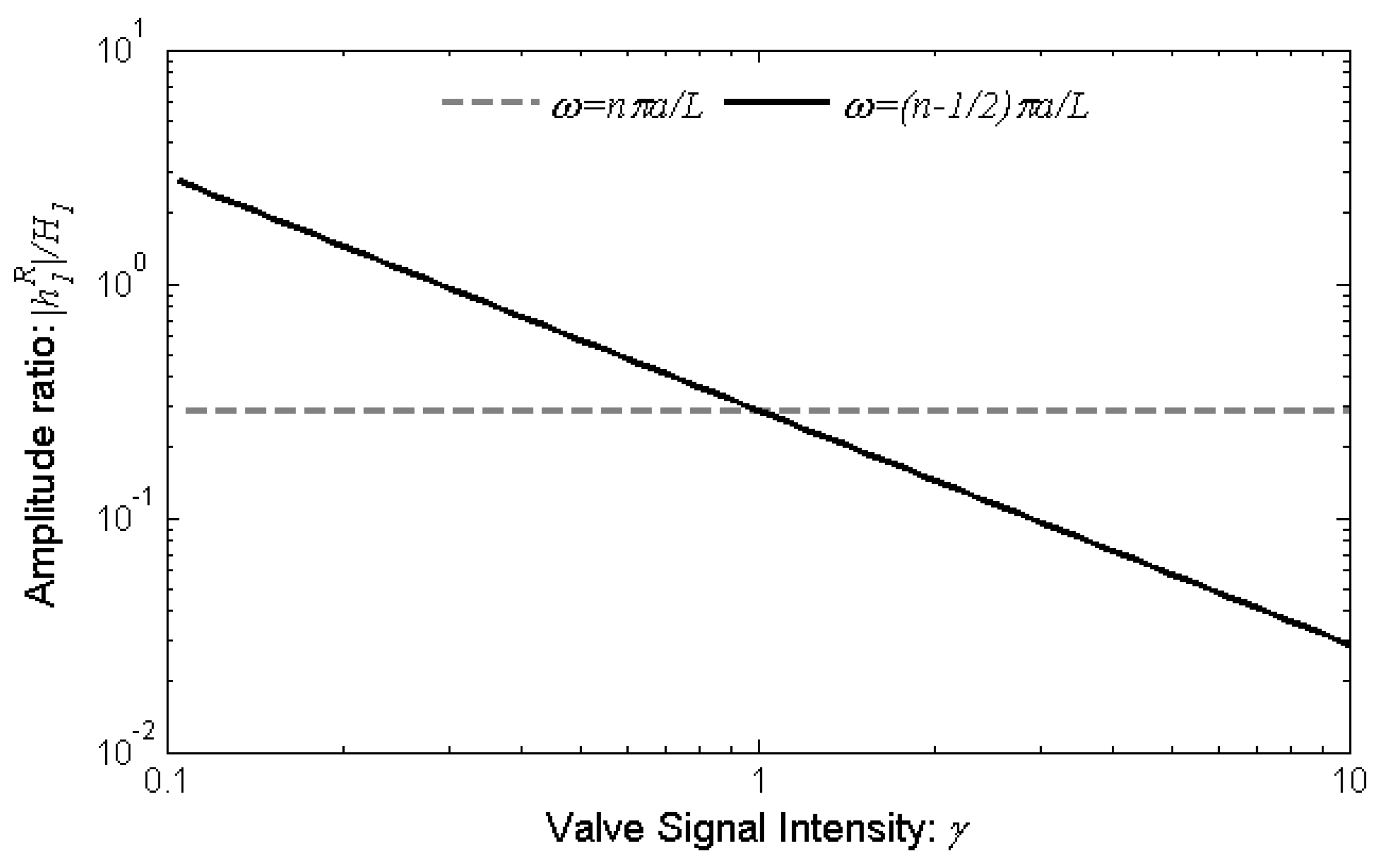
Figure 3 shows the detailed impact of the VSI condition on the upstream pressure fluctuation, which can be summed into three points. First, the gap of the amplitude of pressure fluctuation between the resonances and the anti-resonances declines linearly when the VSI value approaches one. Secondly, the resonance frequencies at condition exchange with the anti-resonant frequencies when . Thirdly, the amplitudes at resonances obtain the minimum at VSI condition , where the pressure fluctuation is the same at any frequency.
3.3. Steady and Unsteady Friction Models
The friction effect acts as a key factor for transient wave propagation in pipelines, and lots of friction models are used in the study of the reservoir–pipe–valve system [16,22,25,36]. The steady friction model is evaluated with the Darcy–Weisbach friction factor, which has a mean effect on the pressure head along the pipe, while the unsteady friction model is proved to be related to the frequency that more reduction is generated at a higher frequency. Furthermore, the effects of friction on the system frequency response applied to the detection of objects in a pipeline are discussed, such as discrete leakages by Lee et al. [16] and extended blockage by Duan et al. [25]. The former studies focused on the pressure fluctuation at the outlet where they send and measure the data. In this part, the pressure fluctuation at both the inlet and the outlet are calculated in the frequency domain, and both the steady friction model and the unsteady friction model are also applied.
With a steady friction model, the upstream and the downstream pressure fluctuations are obtained from Equations (1) and (4)
Since the Darcy–Weisbach friction factor is very small (), the variable relation can be obtained in the defined pump–pipe–valve system; thus the expansion in power series of the square root () allows approximations by ignoring the second and higher orders as
with
Based on the definition, the VSI can be calculated in friction model as follows:
It is found that the steady friction model yields a small decrease of the VSI value which is related with the frequency, though the is independent on the frequency. Nevertheless, the influence becomes weak at high frequency.
Thus, the resonances and anti-resonances for the upstream pressure fluctuations are obtained with the VSI conditions:
- (1)
- If , then and
- (2)
- If , then and
- (3)
- If , then and
Being different with the frictionless model, the resonances and anti-resonances of downstream pressure fluctuations are also found to be related with the VSI, which are represented as
The approximate calculation for the extremums of pressure fluctuation indicates that the steady friction distinctly affects the magnitude of pressure fluctuation but hardly shifts the frequencies of the resonances.
Actually, the steady friction yields a decrease of the maximums at resonances and an increase of the minimums at anti-resonances. Thus, the variation ratios of extremums can be calculated by
where is the variation of minimum pressure fluctuation at the anti-resonances of the downstream side.
The Darcy–Weisbach steady friction model describes the friction from the internal face of the pipe with a friction factor being independent on the frequency; thus the extremums’ variations are scarcely dependent on the frequency. The conclusion is similar with the friction’s influence on the reservoir–pipe–valve system that it is verified to be too small to be neglected on the resonance frequency shift [25,36]. Nevertheless, the former derivation is obtained on the condition of ; thus, the approximation has big errors at low frequency according to the definition in Equation (16). These corollaries are also verified by the next example.
However, experiments have shown that energy losses in the pipeline depend on the frequency of the transient signal whereas the energy increases at higher frequencies, which exceeds the coverage of the Darcy–Weisbach steady friction model. In order to describe the friction effect more accurately, an unsteady friction model is developed by relating with frequency and state of flow [38]:
where is shear decay coefficient with ; is Reynolds number and is kinematic viscosity. Then, it can be rewritten as follows in the forms of complex exponential function,
Thus, the total friction in steady oscillatory flow is expressed as a steady component plus an unsteady component.
Similar to Equation (17), the amplitudes of pressure heat fluctuation at the upstream and the downstream are calculated by the approximation on the condition of ,
with and .
The vital VSI value and the extremums of resonances and anti-resonances can also be calculated by Equations (18)–(25), with the substitution parameters and , but frequencies of the resonances and anti-resonances have made a certain shift by multiplying for each order comparing with those of the steady model.
It is noted that the unsteady friction model leads to a greater decrease of the amplitude of the pressure fluctuation at higher frequency according to Equations (19)–(25) and (33), which correspondes to the practical phenomenon.
In a sum, for the frequency response of the pump–pipe–valve system, the steady friction model has certain effects on the amplitudes of pressure fluctuation but ignores the impact on the frequency shift of resonances, whereas the unsteady friction model distinctly affects both of them.
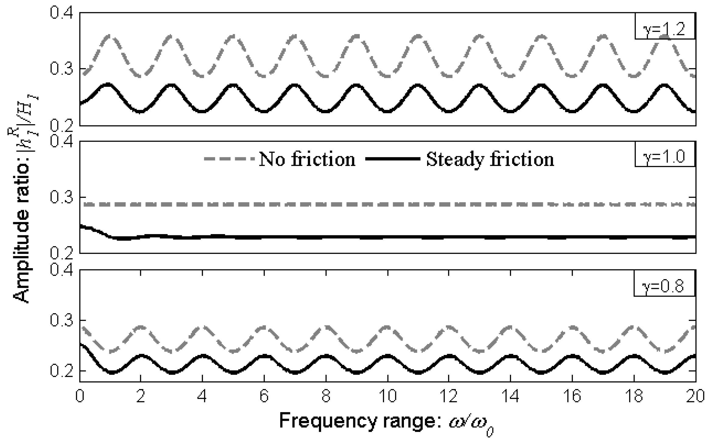
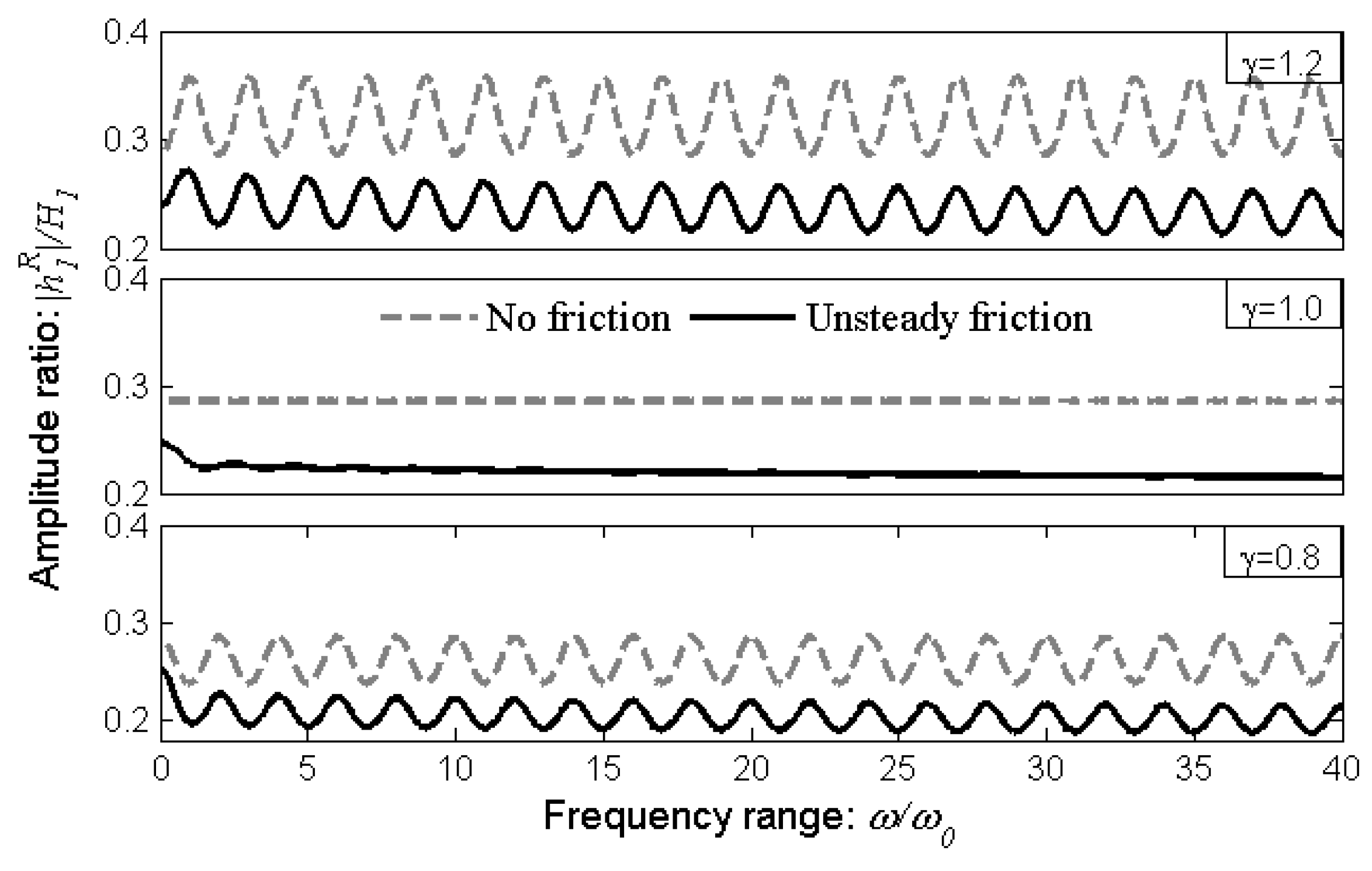
In order to demonstrate the impact of friction on the frequency response, the numerical calculation is performed on the same pipeline with the steady friction model () and with the unsteady friction model (water, 25 °C, ). The frequency spectrum of amplitudes of upstream pressure fluctuations are illustrated in Figure 4 and Figure 5, with three different VSI conditions: , , and . It is clear shown that a constant decrease of the amplitudes is caused by the steady friction model at whatever the VSI conditions, except at very small frequencies (). As shown in Figure 5, the unsteady friction leads to a continuous decrease of the oscillation amplitude with the increase of frequency, and the result is independent on the VSI condition.
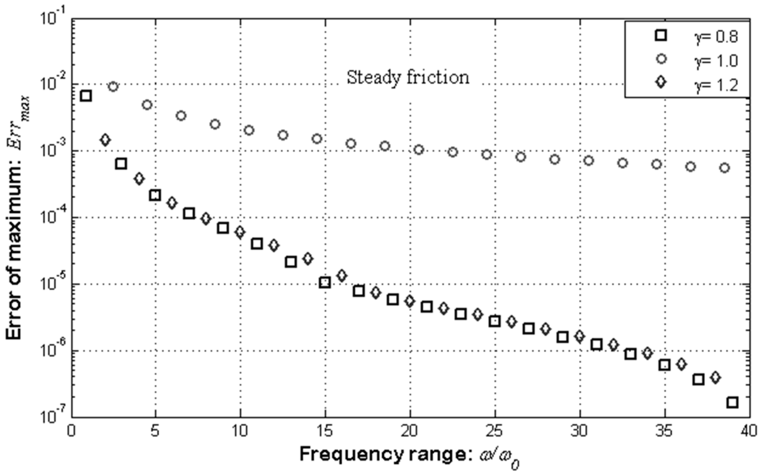
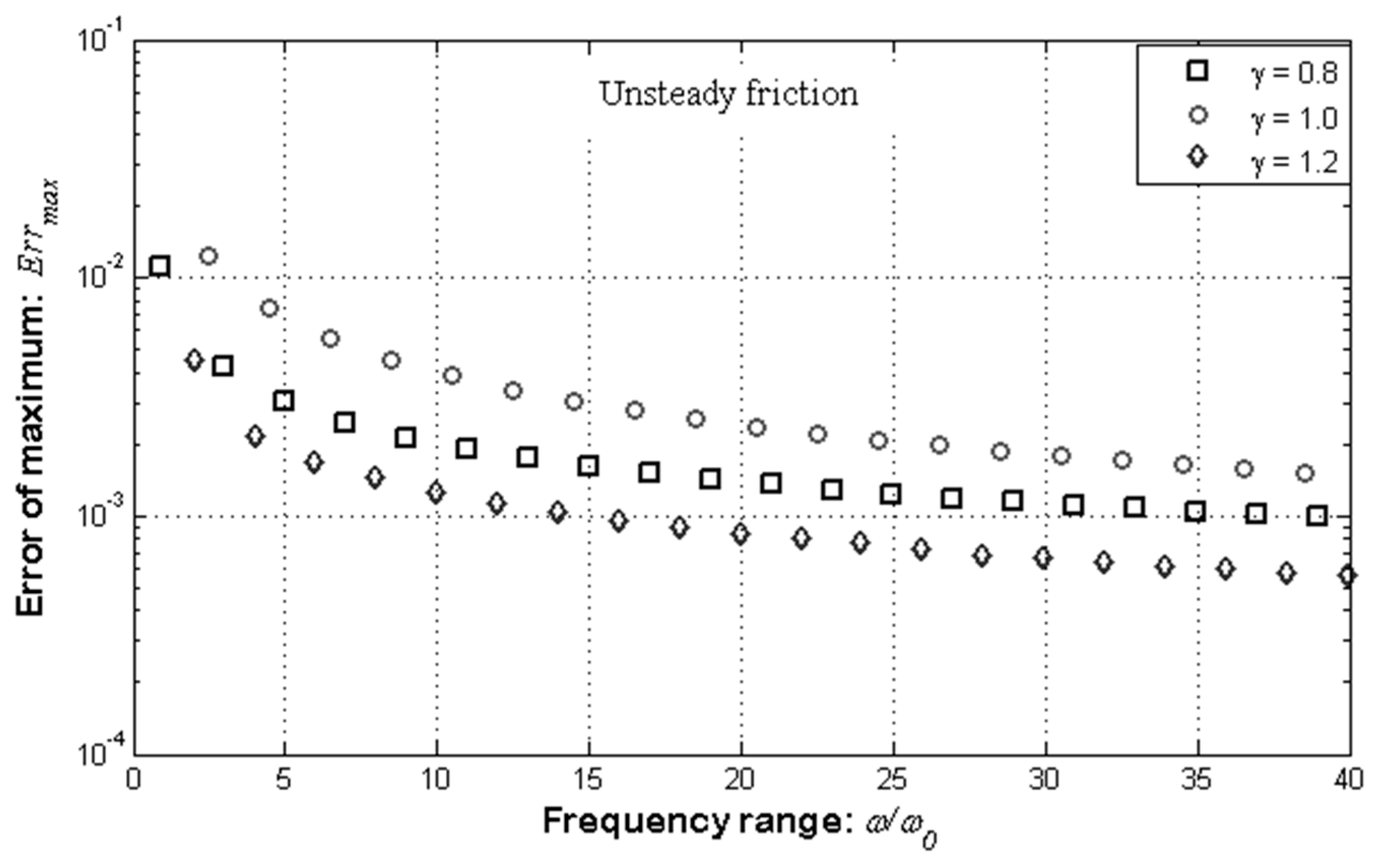
The amplitudes of upstream pressure fluctuation in Figure 4 and Figure 5 are obtained by the actual frequency response (Equation (16)). Errors of extremums between the approximation and the actual values are also considered. The approximation error can be calculated by
and the results are shown in Figure 6 and Figure 7 for the steady friction model and the unsteady friction model, respectively. The approximation errors become smaller when the frequency increases and the biggest values are all smaller than 0.01 for both models. Furthermore, the errors with VSI condition are much bigger than the other two for both models, and the approximation errors for the unsteady friction model are much bigger than those for the steady model at the same VSI condition. Thus, the approximation errors verified a remarkable accuracy of the extremums prediction, and the unsteady friction model has more complicated influences on the frequency response than the steady friction model.
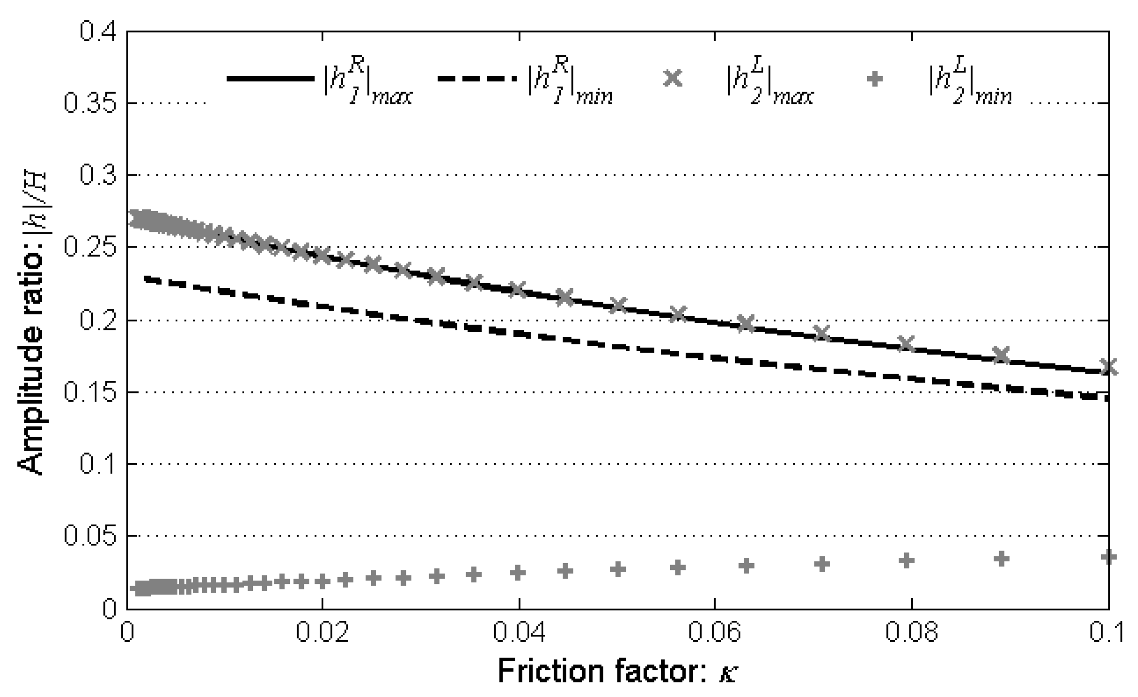
Detailed impacts of the steady friction model on the pressure fluctuation of resonances and anti-resonances are introduced in Figure 8. With the growth of the Darcy–Weisbach friction factor, the resonances amplitudes of the pressure fluctuations at both upstream and downstream sides decrease, as well as anti-resonances at the upstream side, whereas those of anti-resonances at downstream side obtain an almost linear increase. Furthermore, it is noted that the friction has a benefit on the decrease of the differences between the magnitudes of the resonances and anti-resonances in the whole pipeline.
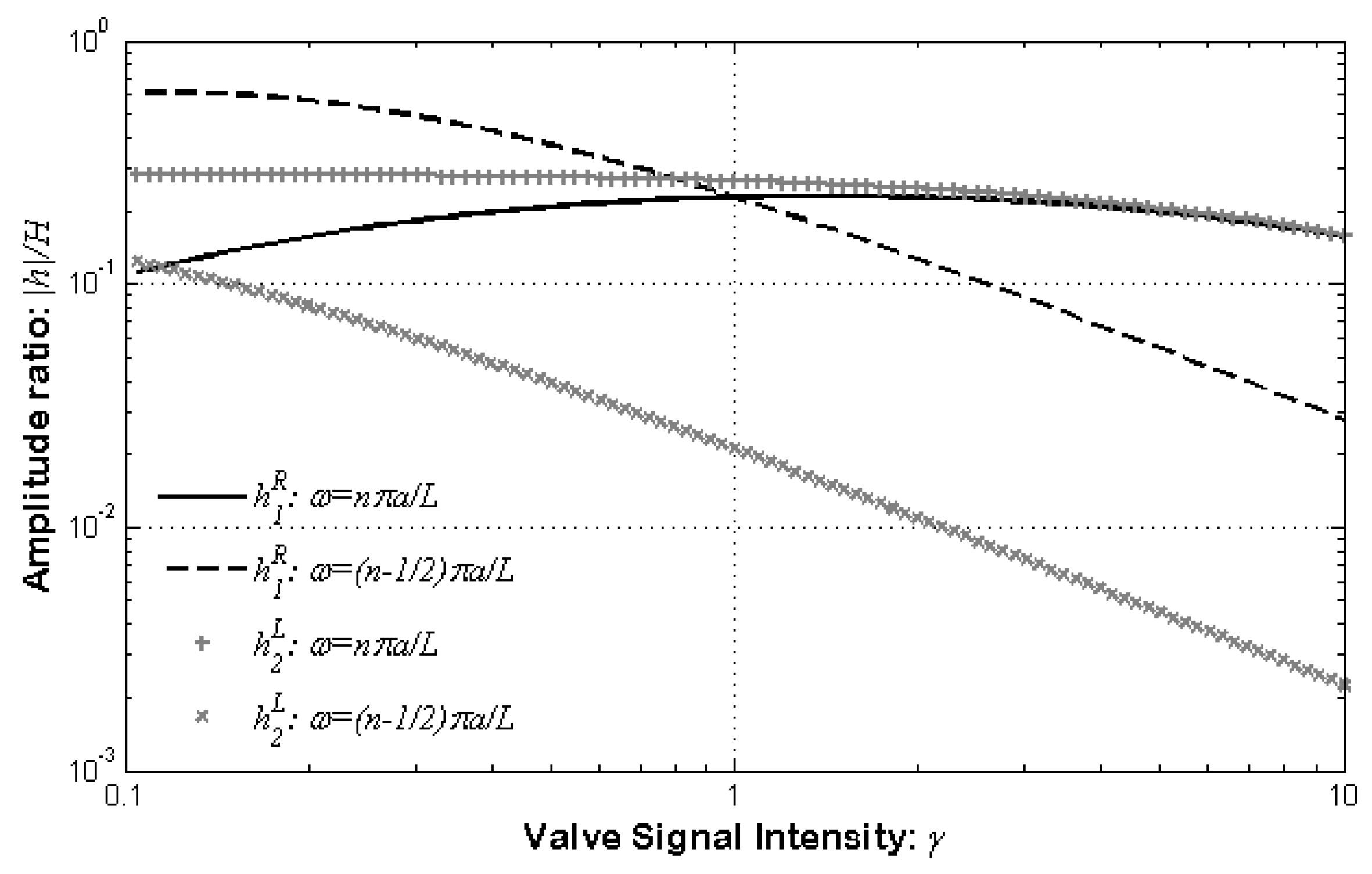
Detailed impacts of the VSI conditions with the steady friction model on the extremums of pressure fluctuations amplitudes (Equations (19–25)) are shown in Figure 9. When the VSI is increasing from to , the pressure fluctuations amplitudes at frequencies decline sharply at both the upstream side and downstream side, whereas those at frequencies fall after a rise at the upstream side and fall after holding at the downstream side. Compared to Figure 3, the upstream pressure fluctuations are affected by the friction but still have a reduction of the difference between the maximum and the minimum of amplitude when approaching to the VSI condition , whereas the downstream pressure fluctuations have a dramatic enlargement of the difference as the VSI condition increasing. Thus, both large pressure fluctuation at the inlet and small pressure fluctuation at the valve can be obtained with the smaller VSI condition, which benefits the control strategy of the ending valve and the upstream signals.
4. Discussion
The frequency response of the pump–pipe–valve system is calculated and analyzed at the upstream and downstream sides, and it is found to be dependent on the friction model and the VSI condition, while the latter can be seen as a combination parameter of flow state and dynamic factor.
For the steady friction effects, an approximate calculation of the resonances and anti-resonances is expressed by Equations (19)–(25) with good accuracy, and it yields to the invariable extremums and resonant frequencies. The unsteady friction model is applied as well, and, further, decrease of the pressure fluctuation at a higher frequency results. It is noted that the nonlinearity of friction model is still a challenging factor for the frequency response of 1D water hammer when applied to practical problems since the high order terms will make non-negligible contributions at some specific conditions [38,39,40]. Duan et al [39] proposed a two-step analytical extension for the friction factor to consider the nonlinear turbulent friction term. The numerical results showed that the contribution of the nonlinear steady friction term to the total frictional damping was highly dependent on the ratio of the generated transient intensity to the initial pipe discharge, which provided a factor to estimate the importance of the nonlinearity on the system frequency response analysis. Creaco [40] used an unsteady friction model to simulate the hydraulic process in a water-distributed network and found that it needed a long time step to obtain the effective signal of pressure head after valve variation. Nevertheless, a precise unsteady model is still needed when applied to practical problems.
As seen from the analysis and calculation, the VSI condition indicates the ability to transfer pressure oscillation from the ending valve to the upstream side; thus, it is linked with the quality of pipeline communication when the pressure oscillation is used as the communicating signals. As defined in Equations (7) and (18), the VSI is dependent on plenty of parameters in the system, among which the mean head loss across the valve is related with the mean discharge, and hence the VSI can be calculated by
Equation (35) provides an effective guiding principle to adjust the VSI condition, where the left equation is based on the invariable flow discharge, while the right equation is supported by the invariable head loss across the valve. In particular, for the pipeline, the smaller cross-section of the pipe will result in a smaller VSI, whereas the wave speed and friction of internal walls have inverse effects. As for the ending valve, the discharge coefficient and the area of the mean opening are inversely proportional to the VSI. In the pump–pipe–valve system, increasing the discharge from the pump has the same effect as the increase of pressure head in the pipe, which leads to the bigger VSI.
The transient waves used as communicating signals in the pump–pipe–valve system usually have requests on the signal intensity and the frequency range; thus, we should balance amplitudes of the pressure fluctuations and differences between resonances and anti-resonances to obtain high quality of communication. As seen from Equations (19)–(25), the bigger magnitude of the valve motion can lead to bigger amplitudes of pressure fluctuations. Then, the smaller value of and , caused by smaller friction factor or shorter pipe, can result in more intense oscillation, which is a similar tendency caused by the smaller VSI. However, the nonuniformity of the amplitudes increases sharply when VSI becomes smaller than one or bigger than one, as seen in Figure 3 and Figure 9. In sum, in order to obtain effective communication by periodic transient waves, making the VSI smaller than one can strengthen the amplitudes at the upstream side, while making the VSI equal to one can provide a unique amplitude for all the frequency. Besides, using a pipe of smooth internal walls is always an effective selection.
5. Conclusions
Being different from the reservoir–pipe–valve system, the frequency response of the pump–pipe–valve system with a constant flow input is analyzed by the system transfer matrix analysis method, and the resonances and anti-resonances of the pressure fluctuations are found to be different between the upstream side and the downstream side. The parameter of the valve signal intension is proposed to distinguish the situations of the frequency response. When the VSI is bigger than one, the upstream pressure fluctuations have the same amplitudes and frequencies of resonances with those at downstream side, but when the VSI is smaller than one, the anti-resonances at upstream side have the same amplitudes and frequencies with resonances at downstream side, while the resonances at upstream side have much bigger amplitudes. Furthermore, the upstream pressure fluctuation has a uniform amplitude at any frequency when the VSI equals one. Thus, the VSI value can be used to predict the intensity of pressure fluctuation along the pipeline.
The friction models are applied to the analysis, and it is found that the steady friction only declines the amplitudes of the pressure fluctuation with a constant value, whereas the unsteady friction results in an expanding reduction of the amplitudes with frequency and an almost constant frequency shift of resonances. Compared to the frictionless model, increasing of the VSI from 0.1 to 10 causes the decrease after an increase for the pressure fluctuation at the upstream side with the friction model, and that the VSI equals one also provides a constant influence on the frequency response.
In order to obtain qualified wave transmission in the pump–pipe–valve system, the larger opening of the valve motion and the smaller friction effects are necessary, but the VSI condition smaller than one or equal to one should be more important. By adjusting the magnitudes of the initial pressure head or constant discharge, the VSI condition is changed, and it is an effective approach to control the behavior of frequency response. Furthermore, investigation of the VSI condition with sudden-changed conduit could also be performed, and it will be discussed in the future.
Author Contributions
For research articles with several authors, a short paragraph specifying their individual contributions must be provided. The following statements should be used “Conceptualization, Z.L., F.Q. and J.H.; methodology, Z.L. and D.P.; validation, D.P.; formal analysis, Z.L. and J.H.; investigation, D.P. and F.Q.; data curation, Z.L.; writing—original draft preparation, Z.L.; writing—review and editing, D.P., F.Q. and J.H.; supervision, F.Q.; funding acquisition, Z.L. and J.H. All authors have read and agreed to the published version of the manuscript.”, please turn to the CRediT taxonomy for the term explanation. Authorship must be limited to those who have contributed substantially to the work reported.
Funding
This research was funded by the Ministry of Science and Technology of China, grant number 2017YFC0306202 and National Natural Science Foundation of China, grant numbers 51906224, 61601407.
Conflicts of Interest
The authors declare no conflict of interest.
References
- Schroeder, M.R. Determination of the geometry of the human vocal tract by acoustic measurements. J. Acoust. Soc. Am. 1967, 41, 1089–1100. [Google Scholar] [CrossRef] [PubMed]
- Mermelstein, P. Determination of the vocal-tract shape from measured formant frequencies. J. Acoust. Soc. Am. 1967, 41, 1283–1294. [Google Scholar] [CrossRef] [Green Version]
- Qunli, W.; Fergus, F. Estimation of blockage dimensions in a duct using measured resonance frequency shifts. J. Sound Vib. 1989, 133, 289–301. [Google Scholar] [CrossRef]
- Qunli, W. Reconstruction of blockage in a duct from single spectrum. Appl. Acoust. 1994, 41, 229–236. [Google Scholar] [CrossRef]
- De Salis, M.H.; Oldham, D.J. Determination of the blockage area function of a finite duct from a single pressure response measurement. J. Sound Vib. 1999, 222, 180–186. [Google Scholar] [CrossRef]
- De Salis, M.H.; Oldham, D.J. The development of a rapid single spectrum method for determining the blockage characteristics of a finite length duct. J. Sound Vib. 2001, 243, 625–640. [Google Scholar] [CrossRef]
- Çelik, H.; Cankurtaran, M.; Cakmak, O. Acoustic rhinometry measurements in stepped-tube models of the nasal cavity. Phys. Med. Biol. 2004, 49, 371–386. [Google Scholar] [CrossRef] [PubMed]
- Fredberg, J.J.; Wohl, M.E.; Glass, G.M.; Dorkin, H.L. Airway area by acoustic reflections measured at the mouth. J. Appl. Physiol. 1980, 48, 749–758. [Google Scholar] [CrossRef] [PubMed]
- Brooks, L.J.; Castile, R.G.; Glass, G.M.; Griscom, N.T.; Wohl, M.E.; Fredberg, J.J. Reproducibility and accuracy of airway area by acoustic reflection. J. Appl. Physiol. 1984, 47, 777–787. [Google Scholar] [CrossRef]
- Sharp, D.B.; Campbell, D.M. Leak detection in pipes using acoustic pulse reflectometry. Acta Acust. United Acust. 1997, 83, 560–566. [Google Scholar]
- Sharp, D.B. Increasing the length of tubular objects that can be measured using acoustic pulse reflectometry. Meas. Sci. Technol. 1998, 9, 1469–1479. [Google Scholar] [CrossRef]
- Chaudhry, M.H. Applied Hydraulic Transients, 3rd ed.; Springer: Berlin/Heidelberg, Germany, 1987; pp. 249–326. [Google Scholar]
- Lee, P.J.; Vitkovsky, J.P.; Lambert, M.F.; Simpson, A.R.; Liggett, J.A. Frequency domain analysis for detecting pipeline leaks. J. Hydraul. Eng. 2005, 131, 596–604. [Google Scholar] [CrossRef] [Green Version]
- Mpesha, W.; Chaudry, M.N.; Gassman, S. Leak detection in pipes by frequency response method. J. Hydraul. Eng. 2001, 127, 137–147. [Google Scholar] [CrossRef]
- Ferrante, M.; Brunone, B. Pipe system diagnosis and leak detection by unsteady-state tests: Harmonic analysis. Adv. Water Resour. 2003, 26, 95–105. [Google Scholar] [CrossRef]
- Lee, P.J.; Vítkovský, J.P.; Lambert, M.F.; Simpson, A.R.; Liggett, J.A. Leak location using the pattern of the frequency response diagram in pipelines: A numerical study. J. Sound Vib. 2005, 284, 1051–1073. [Google Scholar] [CrossRef] [Green Version]
- Covas, D.; Ramos, H.; de Almeida, A.B. Standing wave difference method for leak detection in pipeline systems. J. Hydraul. Eng. 2005, 131, 1106–1116. [Google Scholar] [CrossRef]
- Verde, C.; Visairo, N.; Gentil, S. Two leaks isolation in a pipeline by transient response. Adv. Water Resour. 2007, 30, 1711–1721. [Google Scholar] [CrossRef]
- Guillen, M.; Dulhoste, J.F.; Besancon, G.; Rubio, S.I.; Santos, R.; Georges, D. Leak detection and location based on improved pipe model and nonlinear observer. In Proceedings of the European Control Conference, Strasbourg, France, 24–27 June 2014; pp. 958–963. [Google Scholar]
- Mohapatra, P.K.; Chaudhry, M.H.; Kassem, A.A.; Moloo, J. Detection of partial blockage in single pipelines. J. Hydraul. Eng. 2006, 132, 200–206. [Google Scholar] [CrossRef]
- Mohapatra, P.K.; Chaudhry, M.H.; Kassem, A.A.; Moloo, J. Detection of partial blockages in a branched piping system by the frequency response method. J. Fluids Eng. 2006, 128, 1106–1114. [Google Scholar] [CrossRef]
- Sattar, A.M.; Chaudhry, M.H.; Kassem, A. Partial blockage detection in pipelines by frequency response method. J. Hydraul. Eng. 2008, 134, 76–89. [Google Scholar] [CrossRef]
- Lee, P.J.; Vítkovský, J.; Lambert, M.; Simpson, A.; Liggett, J. Discrete blockage detection in pipelines using the frequency response diagram: Numerical study. J. Hydraul. Eng. 2008, 134, 658–663. [Google Scholar] [CrossRef] [Green Version]
- Duan, H.F.; Lee, P.J.; Ghidaoui, M.S.; Tung, Y.K. Extended blockage detection in pipelines by using the system frequency response analysis. J. Water Resour. Plan. Manag. 2012, 138, 55–62. [Google Scholar] [CrossRef]
- Duan, H.F.; Lee, P.J.; Kashima, A.; Lu, J.; Ghidaoui, M.S.; Tung, Y.K. Extended Blockage Detection in Pipes Using the System Frequency Response: Analytical Analysis and Experimental Verification. J. Hydraul. Eng. 2013, 139, 763–771. [Google Scholar] [CrossRef]
- Meniconi, S.D.; Duan, H.F.; Lee, P.J.; Brunone, B.; Ghidaoui, M.S.; Ferrante, M. Experimental investigation of coupled frequency and time-domain transient test-based techniques for partial blockage detection in pipelines. J. Hydraul. Eng. 2013, 139, 1033–1044. [Google Scholar] [CrossRef]
- Duan, H.F.; Lee, P.J. Transient-Based Frequency Domain Method for Dead-End Side Branch Detection in Reservoir Pipeline-Valve Systems. J. Hydraul. Eng. 2015, 142, 04015042. [Google Scholar] [CrossRef]
- Duan, H.F.; Lee, P.J.; Che, T.C.; Ghidaoui, M.S.; Karney, B.W.; Kolyshkin, A.A. The influence of non-uniform blockages on transient wave behavior and blockage detection in pressurized water pipelines. J. Hydro-Environ. Res. 2017, 17, 1–7. [Google Scholar] [CrossRef]
- Louati, M.; Ghidaoui, M.S.; Meniconi, S.; Brunone, B. Bragg-type resonance in blocked pipe system and its effect on the eigenfrequency shift. J. Hydraul. Eng. 2018, 144, 04017056. [Google Scholar] [CrossRef] [Green Version]
- Che, T.C.; Duan, H.F.; Lee, P.J.; Meniconi, S.; Pan, B.; Brunone, B. Radial pressure wave behavior in transient laminar pipe flows under different flow perturbations. J. Fluids Eng. 2018, 140, 101203. [Google Scholar] [CrossRef]
- Ranginkaman, M.H.; Haghighi, A.; Lee, P.J. Frequency domain modelling of pipe transient flow with the virtual valves method to reduce linearization errors. Mech. Syst. Signal Process. 2019, 131, 486–504. [Google Scholar] [CrossRef]
- Pan, B.; Duan, H.F.; Meniconi, S.; Urbanowicz, K.; Che, T.C.; Brunone, B. Multistage Frequency-Domain Transient-Based Method for the Analysis of Viscoelastic Parameters of Plastic Pipes. J. Hydraul. Eng. 2020, 146, 04019068. [Google Scholar] [CrossRef]
- Lee, P.J.; Vítkovský, J.P. Quantifying linearization error when modeling fluid pipeline transients using the frequency response method. J. Hydraul. Eng. 2010, 136, 831–836. [Google Scholar] [CrossRef]
- Duan, H.F. Uncertainty analysis of transient flow modeling and transient-based leak detection in elastic water pipeline systems. Water Resour. Manag. 2015, 29, 5413–5427. [Google Scholar] [CrossRef] [Green Version]
- He, S.; Jiao, Z.; Guan, C.; Xu, Y. Research on pulsation attenuation characteristics of expansion chamber in hydraulic systems. In IEEE International Conference on Industrial Informatics, Beijing, China, 25–27 July 2012; IEEE: Piscataway, NJ, USA, 2012; pp. 735–739. [Google Scholar]
- Lee, P.J.; Duan, H.-F.; Ghidaoui, M.; Karney, B. Frequency domain analysis of pipe fluid transient behaviour. J. Hydraul. Res. 2013, 51, 609–622. [Google Scholar] [CrossRef]
- Lee, P.J.; Duan, H.; Tuck, J.; Ghidaoui, M. Numerical and experimental study on the effect of signal bandwidth on pipe assessment using fluid transients. J. Hydraul. Eng. 2015, 141, 04014074. [Google Scholar] [CrossRef]
- Vítkovský, J.P.; Bergant, A.; Lambert, M.F.; Simpson, A.R. Frequency-Domain Transient Pipe Flow Solution Including Unsteady Friction. In Proceedings of the Pumps, Electromechanical Devices and Systems: Applied to Urban Water Management, Valencia, Spain, 22–25 April 2003; pp. 773–780. [Google Scholar]
- Duan, H.F.; Che, T.C.; Lee, P.J.; Ghidaoui, M.S. Influence of nonlinear turbulent friction on the system frequency response in transient pipe flow modelling and analysis. J. Hydraul. Res. 2018, 56, 451–463. [Google Scholar] [CrossRef]
- Creaco, E.; Campisano, A.; Franchini, M.; Modica, C. Unsteady Flow Modeling of Pressure Real-Time Control in Water Distribution Networks. J. Water Resour. Plann. Manag. 2017, 143, 04017056. [Google Scholar] [CrossRef]
Figure 1.
The diagram of the pump–pipe–valve system.

Figure 2.
The frequency responses of a single pipe with the frictionless model at three valve signal intensity (VSI) conditions ().
Figure 2.
The frequency responses of a single pipe with the frictionless model at three valve signal intensity (VSI) conditions ().

Figure 3.
Impact of the VSI conditions on the resonances and anti-resonances of the upstream pressure fluctuation.
Figure 3.
Impact of the VSI conditions on the resonances and anti-resonances of the upstream pressure fluctuation.

Figure 4.
Impacts of the Darcy–Weisbach steady friction model () on the frequency response with three VSI conditions.
Figure 4.
Impacts of the Darcy–Weisbach steady friction model () on the frequency response with three VSI conditions.

Figure 5.
Impacts of the unsteady friction model () on the frequency response with three VSI conditions.
Figure 5.
Impacts of the unsteady friction model () on the frequency response with three VSI conditions.

Figure 6.
Approximation errors of with the steady friction model.

Figure 7.
Approximation errors of with the unsteady friction model.

Figure 8.
Impact of the Darcy–Weisbach friction factor on the resonances and anti-resonances of the upstream and downstream pressure fluctuations at VSI condition .
Figure 8.
Impact of the Darcy–Weisbach friction factor on the resonances and anti-resonances of the upstream and downstream pressure fluctuations at VSI condition .

Figure 9.
Impact of the VSI condition on the resonances and anti-resonances of the upstream and downstream pressure fluctuations with a steady friction model ().
Figure 9.
Impact of the VSI condition on the resonances and anti-resonances of the upstream and downstream pressure fluctuations with a steady friction model ().

© 2020 by the authors. Licensee MDPI, Basel, Switzerland. This article is an open access article distributed under the terms and conditions of the Creative Commons Attribution (CC BY) license (http://creativecommons.org/licenses/by/4.0/).
Share and Cite
MDPI and ACS Style
Liu, Z.; Pan, D.; Qu, F.; Hu, J. Model Analysis and System Parameters Investigation for Transient Wave in a Pump–Pipe–Valve System. Water 2020, 12, 1014. https://doi.org/10.3390/w12041014
AMA Style
Liu Z, Pan D, Qu F, Hu J. Model Analysis and System Parameters Investigation for Transient Wave in a Pump–Pipe–Valve System. Water. 2020; 12(4):1014. https://doi.org/10.3390/w12041014
Chicago/Turabian StyleLiu, Zubin, Dingyi Pan, Fengzhong Qu, and Jianxin Hu. 2020. "Model Analysis and System Parameters Investigation for Transient Wave in a Pump–Pipe–Valve System" Water 12, no. 4: 1014. https://doi.org/10.3390/w12041014
Note that from the first issue of 2016, this journal uses article numbers instead of page numbers. See further details here.