Interplay between Fingering Instabilities and Initial Soil Moisture in Solute Transport through the Vadose Zone


1
Department of Civil Engineering: Hydraulics, Energy and Environment, Universidad Politécnica de Madrid, 28040 Madrid, Spain
2
Department of Earth and Planetary Sciences, University of California Berkeley, Berkeley, CA 94670, USA
3
Department of Civil and Environmental Engineering, Massachusetts Institute of Technology, Cambridge, MA 02139, USA
*
Author to whom correspondence should be addressed.
Water 2020, 12(3), 917; https://doi.org/10.3390/w12030917
Submission received: 11 February 2020
/
Revised: 15 March 2020
/
Accepted: 18 March 2020
/
Published: 24 March 2020
(This article belongs to the Special Issue Groundwater and Contaminant Transport)
Abstract
:Modeling water flow and solute transport in the vadose zone is essential to understanding the fate of soil pollutants and their travel times towards groundwater bodies. It also helps design better irrigation strategies to control solute concentrations and fluxes in semiarid and arid regions. Heterogeneity, soil texture and wetting front instabilities determine the flow patterns and solute transport mechanisms in dry soils. When water is already present in the soil, the flow of an infiltration pulse depends on the spatial distribution of soil water and on its mobility. We present numerical simulations of passive solute transport during unstable infiltration of water into sandy soils that are prone to wetting front instability. We study the impact of the initial soil state, in terms of spatial distribution of water content, on the infiltration of a solute-rich water pulse. We generate random fields of initial moisture content with spatial structure, through multigaussian fields with prescribed correlation lengths. We characterize the patterns of water flow and solute transport, as well as the mass fluxes through the soil column. Our results indicate a strong interplay between preferential flow and channeling due to fingering and the spatial distribution of soil water at the beginning of infiltration. Fingering and initial water saturation fields have a strong effect on solute diffusion and dilution into the ambient water during infiltration, suggesting an effective separation between mobile and inmobile transport domains that are controlled by the preferential flow paths due to fingering.
1. Introduction
Water flow and solute transport through unsaturated soil control the movement and distribution of pollutants in the vadose zone [1] and the contamination of groundwater resources [2,3]. Current important applications include the design of sustainable unconventional irrigation processes [4,5], understanding the transport of colloids [6] and viruses [7,8] through the unsaturated zone, and characterizing the role of pore-scale processes on mixing and dispersion in two-phase [9,10] and three-phase [11] fluid systems. Key mechanisms that determine the distribution of water and solutes in soil include heterogeneity [12], structure and layering [13,14,15], the presence of macropores and their connectivity [16], the presence of vegetation and crops [17], and the particular protocols and water compositions used for irrigation in water-scarce arid and semiarid regions [4,18].
Numerical simulation of multiphase flow in porous media is a powerful tool to understand water flow and solute transport in the unsaturated zone, from the pore scale to the field scale [12,18,19]. Richards’ equation [20,21,22,23,24] and water-balance models [25] have been extensively used for groundwater recharge estimates. The effect of preferential flow or complex water flow patterns on transport processes in the vadose zone has been studied in the framework non-equilibrium transport theories, including dual porosity/permeability models [26,27] based on the Richards equation coupled to advection–dispersion–sorption equation [3,28]. Pore-scale modeling has been used to understand the basic transport mechanisms in unsaturated flow [29,30,31,32]. Field- and catchment-scale models assume stable infiltration fronts, in agreement with the classical predictions of Richards’ equation [20,21,22,23], but in disagreement with experiments. Experimental observations show that preferential flow due to fingering instabilities may significantly influence infiltration into dry sandy soils [33,34,35,36,37], controlling the transport of contaminants to surface and groundwaters [38].
In this paper, we use numerical simulation to study the impact of the initial soil water distribution on solute transport due to the infiltration and redistribution of a saltwater pulse. The patterns of water flow and solute transport are complex in this context, as fingering instabilities interact with the preferential flow paths created by the large water-content areas, due to the nonlinear nature of relative conductivity in unsaturated flow. We simulate coupled unsaturated flow and advection–diffusion of a passive tracer due to an infiltration pulse. We show that the patterns of preferential flow and solute transport and dilution into the ambient preexisting soil water are controlled by the spatial patterns of the distribution of initial pore water. We consider spatial distributions of initial soil water that aim at resembling the structure of soil after several cycles of infiltration and redistribution. To this end, we generate random fields with Gaussian statistics and spatial correlation, characterized by the maximum and minimum saturations and the spatial correlation lengths.
We show that the initial water content and its spatial distribution plays a key role in the patterns of water infiltration and solute transport in unsaturated coarse soil. We characterize the interplay between the fingering instability and the spatial structure of the initial water saturation field, as well as the impact of solute effective dispersivity on the efficiency of solute dilution into the ambient fluid. The effective diffusivity/dispersivity of solute is particularly important for solute dilution in dry soils, or in those where the initial water saturation field induces flow focusing (vertical correlation). When the initial saturation field leads to complex infiltration patterns (the presence of water lenses or isotropic fields with large saturation), the flow field is also complex and enhances mixing leading to more efficient dilution.
The paper is organized as follows. In Section 2, we discuss the mathematical model and its implementation using the finite element method. Section 3 presents an analysis of 1D constant-rate infiltration and solute transport into a soil column, to illustrate the speeds of the water and solute fronts when the soil is initially wet. In Section 4 we describe the generation of random, spatially correlated fields of initial water saturation, which are then used to conduct numerical simulations of infiltration of a saltwater pulse. Finally, we present our concluding remarks in Section 5.
2. Materials and Methods
2.1. Mathematical Model of Unsaturated Flow in Porous Media
We assume a rigid porous medium, and write mass conservation of water in terms of the volume fraction of pore space occupied by it, (mm)—the water saturation:
where is the medium porosity (mm), is the water density (kg m), assumed here to be independent of the solute concentration, is the water mass flux (kg sm), and is the Darcy velocity (m s). In the above expression we do not consider sources or sinks (e.g. evapotranspiration). We assume that the air density in negligible compared to that of water, and that the flow conditions are such that air remains at constant atmospheric pressure. We assume that water is incompressible, and that the mass flux is driven by a Darcy flow potential :
where k is the intrinsic permeability of the soil (m), is the dynamic viscosity of water (Pa s), and is the dimensionless water relative permeability, which accounts for the effect of partial saturation on hydraulic conductivity [20,39,40]. We define the saturated hydraulic conductivity, (m s), as:
where g is the gravitational acceleration (m s). Gravity acts along the vertical coordinate, z (increasing with depth).
The flow potential, (Pa), comprises gravitational and capillary phenomena. It is a second-gradient extension of the Richards model of unsaturated flow [20,41,42,43,44,45]:
The water suction head, (m), is written using Leverett scaling [46]:
where is the characteristic capillary heigth (m), is the Leverett J-function [46]—a dimensionless capillary pressure function—and (m) is the expansion coefficient for the second-gradient theory [45]:
where the function is defined based on the idea of capillary energy from a pressure–saturation relationship [47,48]. We take the characteristic length of the gradient energy term, (m), as proportional to the capillary height, , for which Leverett scaling predicts:
where is the air-water surface tension (N/m), and the static contact angle, which is assumed to be the same throughout the domain. Finally, the conservation of mass equation for water can be written as:
In the above equation, the constitutive relationships , , and , are also nonlinear functions of saturation (see Table 1).
2.2. Transport of a Passive Solute
Neglecting solute adsorption, conservation of mass for the solute is given by the advection–diffusion equation:
where c is the solute concentration in water (kg m), and we assume an isotropic diffusion–dispersion tensor, (ms). Solute is advected by the Darcy velocity from the unsaturated flow equation:
For implementation purposes, we write (9) as:
2.3. Finite Element Implementation
To apply a standard Finite Element (FEM) discretization using elements, we write the model Equation (8) as a system of two second-order equations. Coupled to the solute transport equation, the coupled model can be written as:
The above mixed formulation can be compactly written in vector form as:
where the dependent variables, , and fluxes, , are given by:
respectively. The coupled Equations (12) and (13) are discretized in space using a standard Galerkin formulation with linear elements, and advanced in time using an adaptive implicit scheme (BDF2) [49].
For constant flow-rate infiltration, we impose an inward water volumetric flux at the top boundary, (m s):
where is the flux ratio (dimensionless), which takes a value between 0 and 1. At the bottom boundary we model a natural outflow by imposing the local vertical flux:
All other boundaries are zero-flux. For the conservation of mass of solute, we impose a constant concentration kg/m, and model the free drainage outlflow at the bottom of the domain, , as:
3. Results: One-Dimensional Infiltration Fronts
3.1. Problem Set-Up
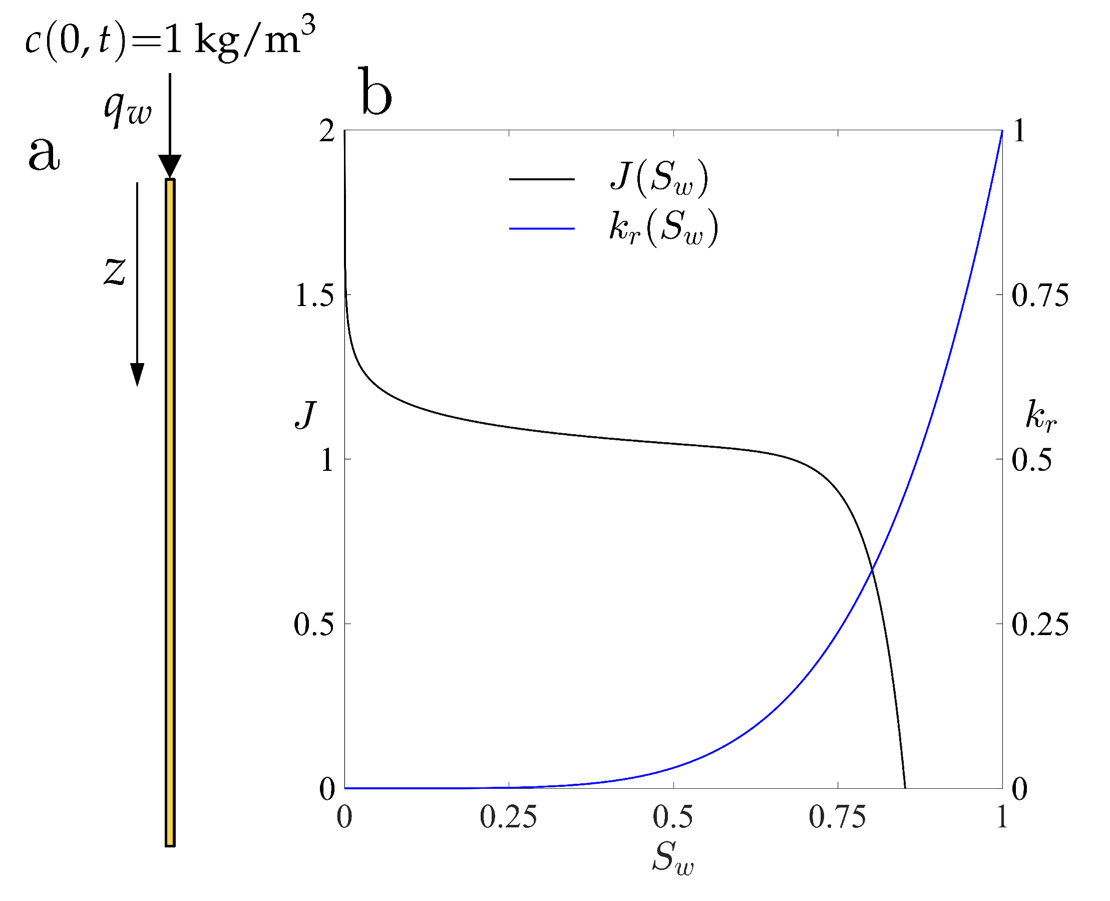
To characterize 1D infiltration fronts in coupled unsaturated flow and transport in a soil column, we simulate constant-rate infiltration into soil with a nonzero initial freshwater saturation (Figure 1a). The initial solute concentration is zero, = 0 and the infiltrating water has a constant solute concentration, = 1 kg/m. We explore solute transport for several infiltration rates and initial water saturations, (Figure 2, Figure 3 and Figure 4).
Capillary pressure and relative permeability functions [41] are based on standard constitutive-relation modeling [50,51] (Figure 1b). We define the Leverett J-function, , as [43]:
where is the Brooks and Corey parameter [50], and >0 and ≥1 control the shape of the function near = 1. The gradient-energy coefficient, , is given by the integral of the J-function, :
The above relationships with ≈1 yield convex capillary energies and prevent the water saturation from taking unphysical values above 1 [45].
The relative permeability, , is a convex function of saturation [41]. The Brooks–Corey [50] and van Genuchten [51] models are often used. Here we set:
with a>1. The effective or reduced water saturation, , is defined in terms of the irreducible water saturation, .
The model equations for the 1D problem simplify to (infiltration along a vertical coordinate z):
The Darcy advection velocity can be identified as:
We consider a soil column of height H = 1 m, uniformly discretized using 5000 finite elements. The soil porosity is constant and homogeneous, = , as are the fluid density and viscosity, = 1000 kg/m and = Pa·s. The constitutive parameters are: a = 5, = 10, = 40, = 1, and = 0. The capillary height and are = = 2 cm. The saturated hydraulic conductivity is = 40 cm/min, and the infiltration rate, , is reported as a flux ratio, = /. For simplicity, we set a contant form of in these 1D simulations, = . The effective diffusivity is = m/s.
3.2. Impact of the Initial Saturation on Solute Transport
We estimate the advection speed of the water and solute fronts by assuming a Richards flow model without capillary pressure effects (the hyperbolic limit of (23)):
For constant-rate infiltration into soil with initial saturation and solute concentration , the speeds of the water and solute fronts, and (m s), are given by:
where the left saturation state, , is such that the infiltration flux is = , and the infiltrating water has solute concentration . For infiltration into freshwater ( = 0), the solute front speed reduces to:
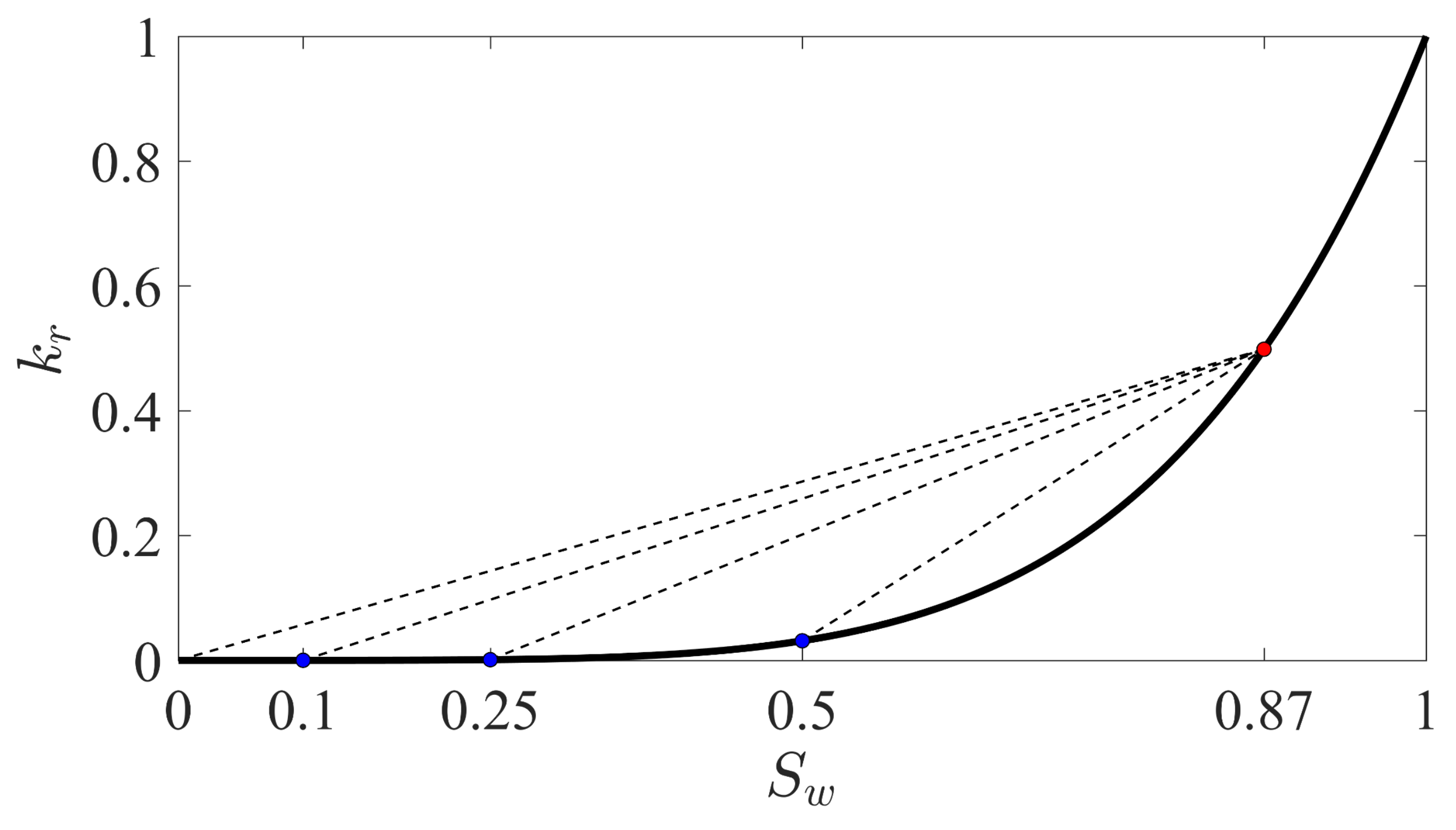
The graphical interpretation of Equations (29) and (30) is shown in Figure 2: for a given infiltration rate, which leads to a left saturation state , the speed of the water infiltration front is proportional to the slope of the secant line from the relative mobility evaluated at the initial saturation, (blue dots), to the relative mobility evaluated at the infiltrating saturation, (red dot). When the initial concentration is zero, the solute front propagates with a speed that is proportional to the slope of the secant line from zero to . These results imply that the water front is faster than the solute front.
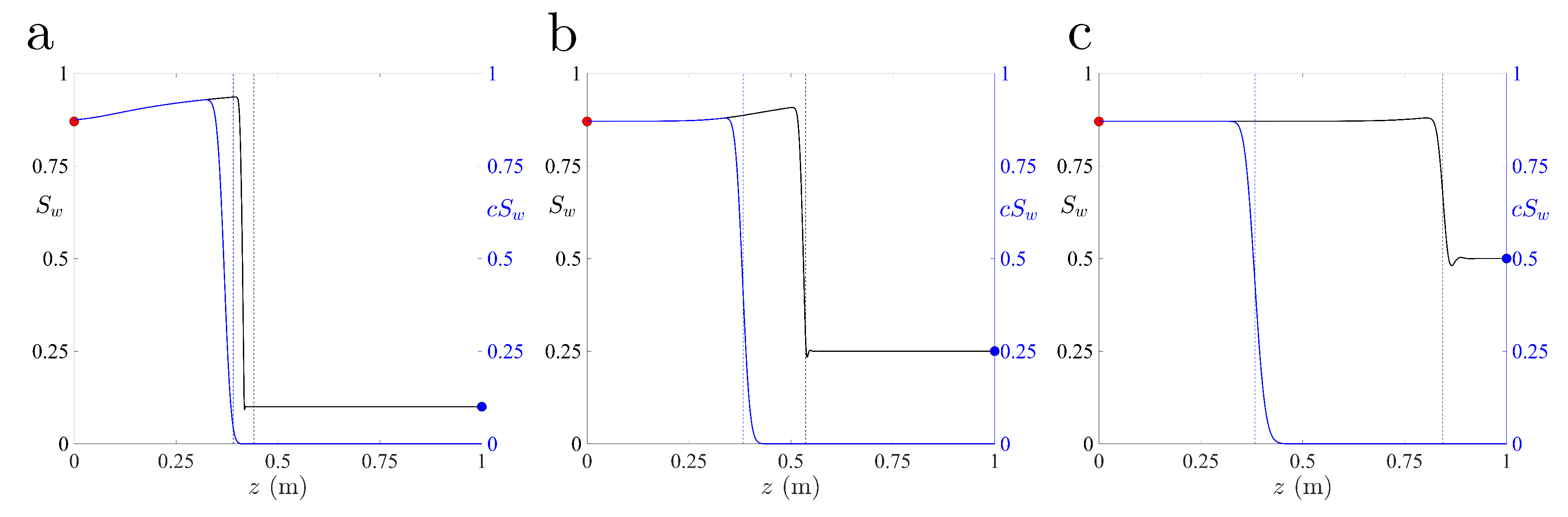
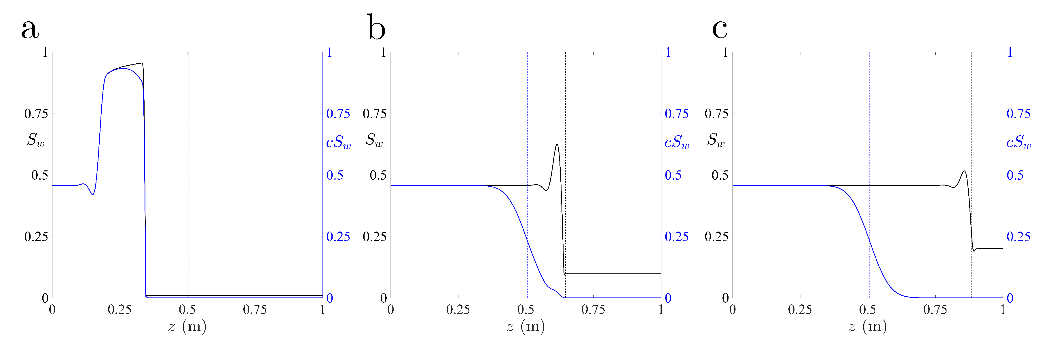
To confirm this behavior, we compare the 1D profiles of water saturation and solute concentration during infiltration, for the same flux ratio = and three initial saturations, = , and (Figure 3). We also compare results with a flux ratio = , and initial saturations, = , and (Figure 4). As predicted by the analytical result (29), the water front is faster than the solute front, and the difference in speeds increases with initial saturation, so that the change in water flux at the outlet due to infiltration arrives faster than the solute flux. The predictions from Equations (29) and (30) are not strictly valid for the full model (23), as evident by the mismatch between simulated front (solid lines) and predicted front (dashed lines) in Figure 3 and Figure 4. This is because of the saturation overshoot induced by the fourth-order term, which leads to an overshoot in solute content for infiltration into dry soil. The impact of the fourth-order term disappears as the initial saturation (and hence the saturation overshoot) increases, so that the hyperbolic model predicts the front positions accurately (Figure 3c and Figure 4c).
4. Results: Two-Dimensional Infiltration Patterns
4.1. Problem Set-Up
We simulate the infiltration and redistribution of a saltwater pulse in a two-dimensional domain (Figure 5). The soil is not dry at the beginning of the simulation, but rather has a random, spatially correlated initial fresh water saturation that resembles the state of the soil after several cycles of infiltration and redistribution (Figure 5a). The domain is a square of size 1 m × 1 m, which is discretized using a 500 × 500 Cartesian grid. The soil porosity is assumed to be constant and homogeneous, = , as are the fluid density and viscosity, = 1000 kg/m and = Pa·s, respectively. The constitutive parameters are: a = 7, = 10, = 40, = 1, and = . In the definition of the capillary height, we set = = 2 cm. The soil is assumed to be homogeneous in terms of permeability, with a saturated hydraulic conductivity = 40 cm/min (see Table 1).
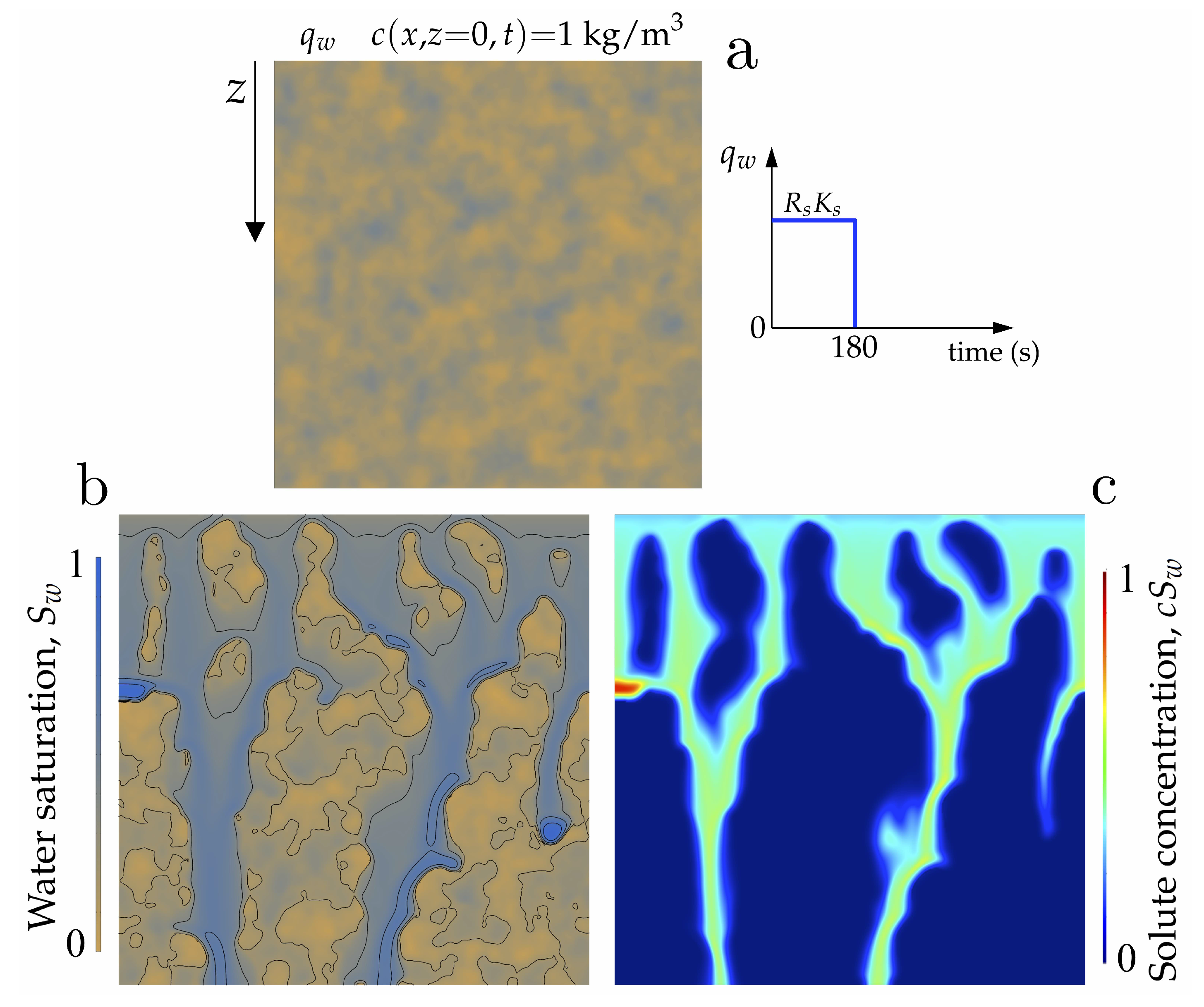
The initial distribution of soil water is heterogeneous, and we simulate an infiltration pulse with nonzero solute concentration (Figure 5a). The initial solute concentration is zero, and the pulse is implemented as constant-flux infiltration during a short time period. The solute concentration remains constant at the top boundary, = = 1 kg/m. We simulate the coupled unsaturated flow and solute transport dynamics, and study the impact of initial soil moisture distribution on the solute flux at the bottom of the domain, and dilution of the solute over the domain. At the top boundary we impose a flux ratio = for the first 180 s, so that the inward volumetric flux is given by = < 180 s) = .
We generate multi-Gaussian fields of initial saturations, in the range between and and correlation lengths and . As main field variables we compute the water saturation, , and solute concentration, c, and study the patterns of water infiltration (Figure 5b) and solute concetration, (Figure 5c), depending on the structure of the initial saturation field and effective diffusivity, . Further details on the generation of random correlated fields are given in Section 4.2 below, and a summary of model parameters and constitutive definitions is given in Table 1.
4.2. Statistics of the Initial Water Saturation Fields
The initial saturation field is a random, spatially correlated function of space, (Figure 6 and Figure 7). To simplify the parametrization of these random fields, we specify the correlation lengths, and , and the maximum and minimum initial saturations, and . We begin by generating random correlated fields, , with zero mean and unit standard deviation, using the classical algorithm by Gelhar and Axness [52]. The function yields the basic spatial structure of the intial saturation field. The actual saturations are then obtained by rescaling according to the target maximum and minimum values, as:
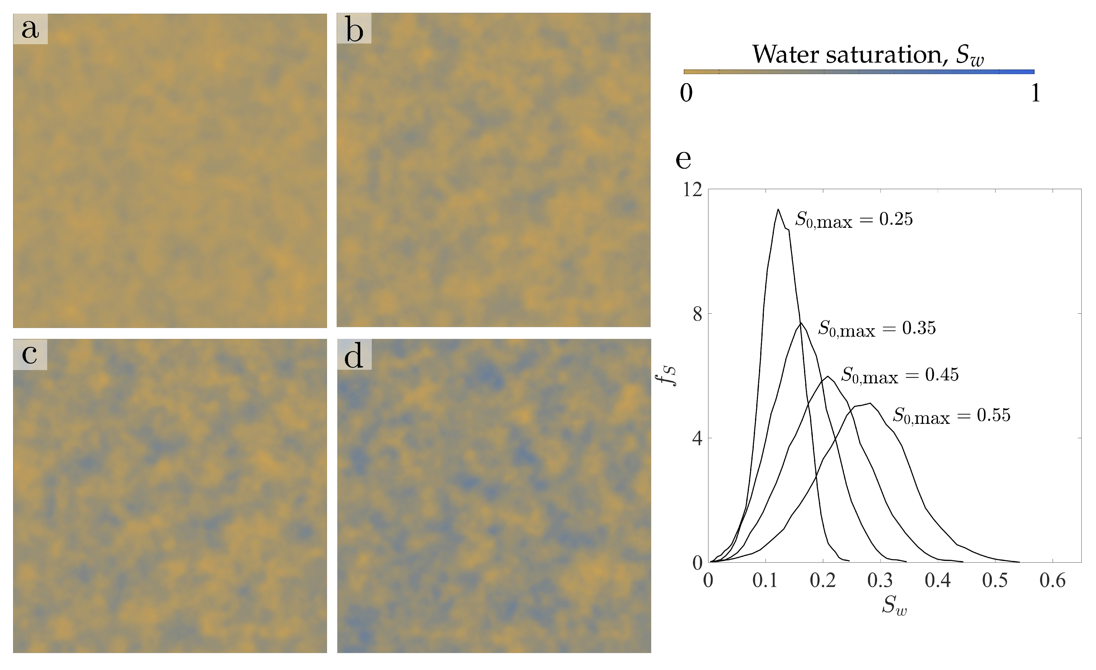
Some examples of isotropic ( = ) water saturation fields obtained with the above procedure are shown in Figure 6, along with their sample probability density functions. The minimum initial saturation is the same in all cases, = , as is the correlation length, = cm. The maximum initial saturations vary between = and = . The probability density functions flatten and increase their mean as increases.
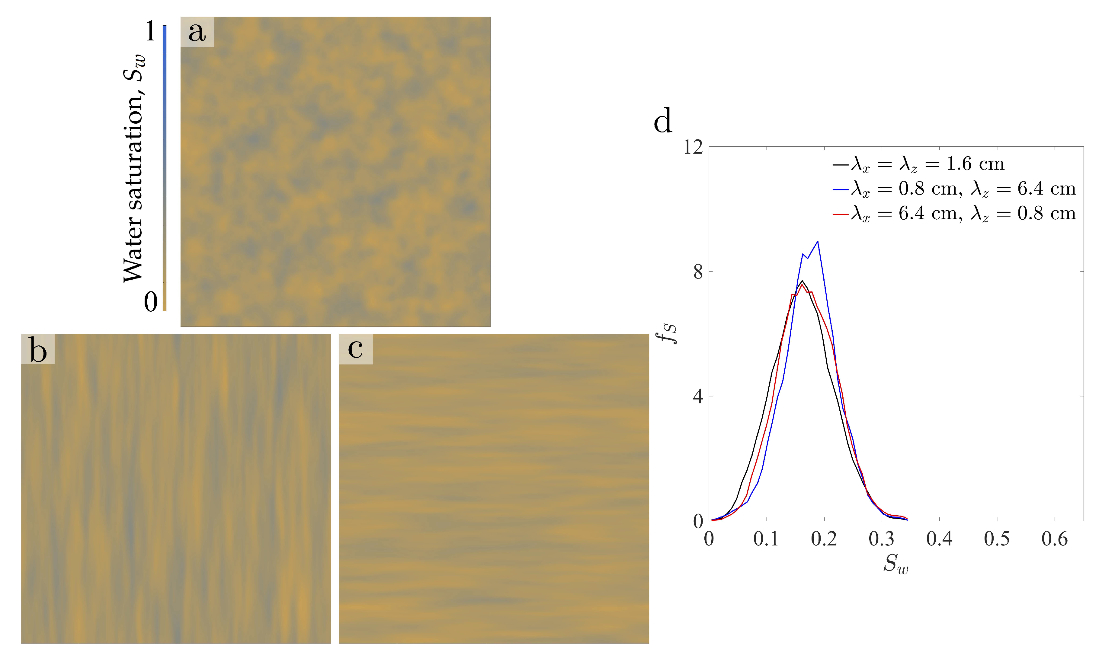
We also show sample realizations of anisotropic saturation fields (Figure 7), with minimum initial saturation = , and various maximum saturations, . We show sample fields with = , and correlation lengths = = cm, = cm, = cm, and = cm, = cm. The sample probability distributions are essentially the same in all cases (Figure 7).
4.3. Sample Two-Dimensional Simulations
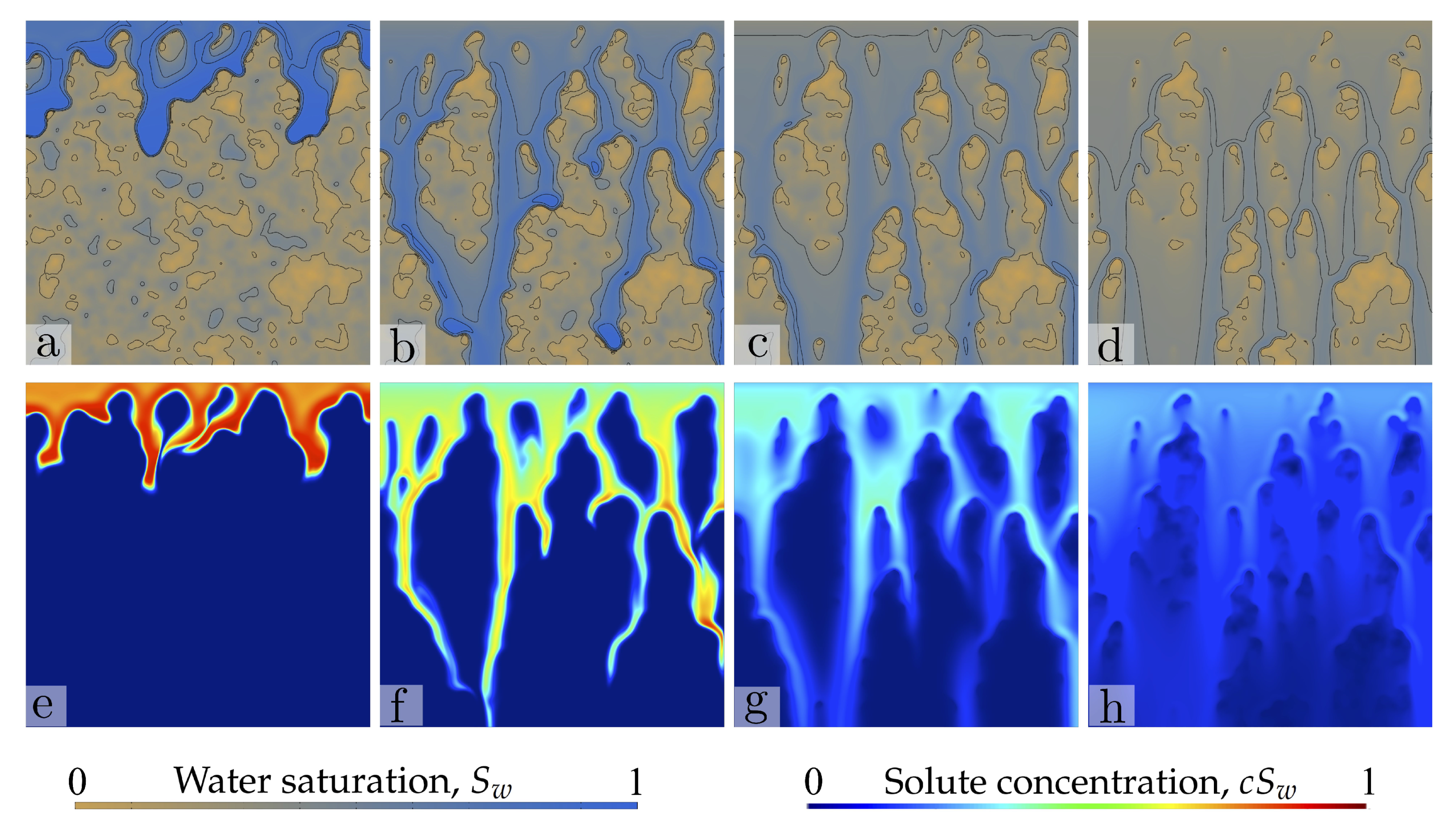
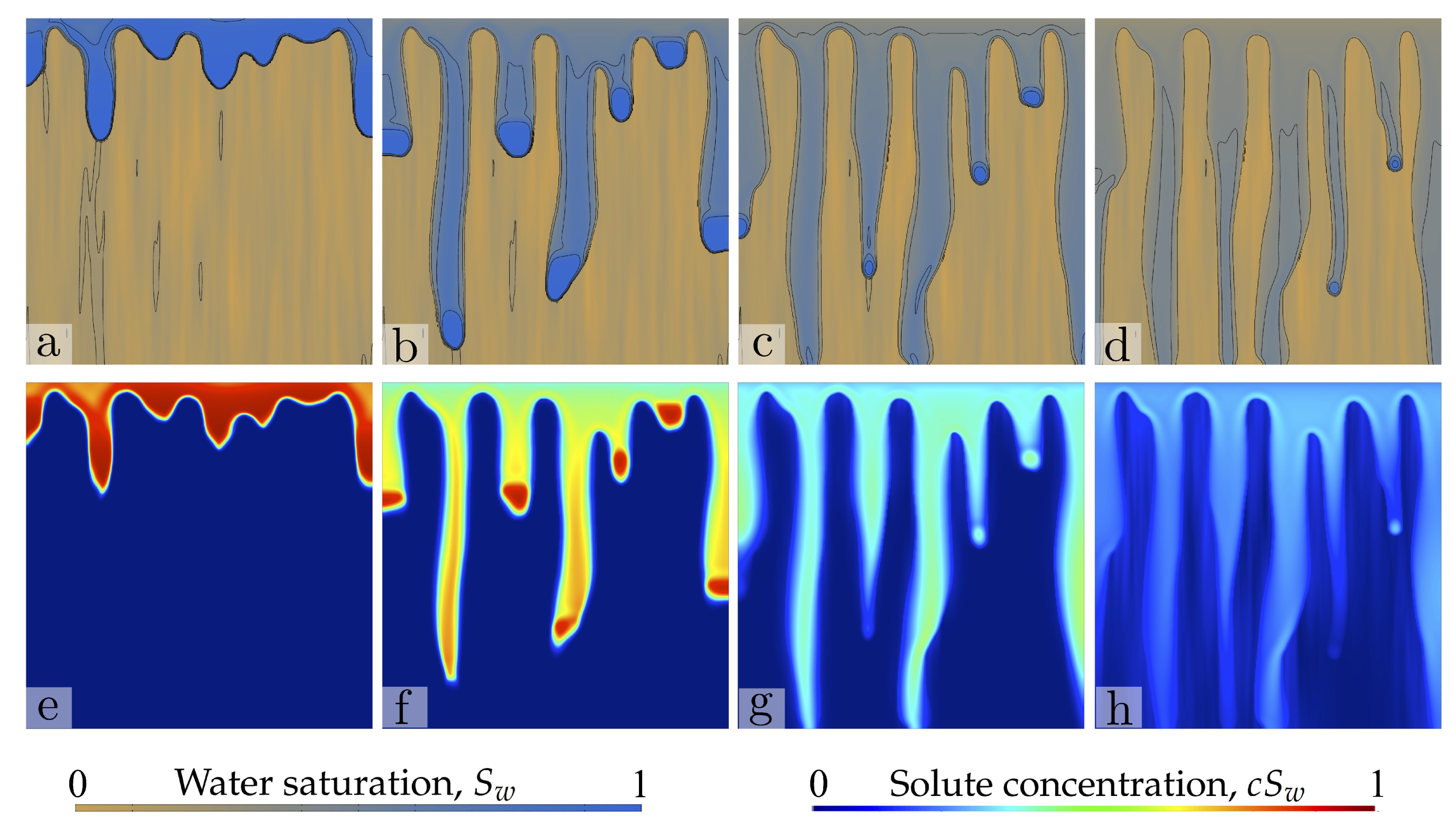
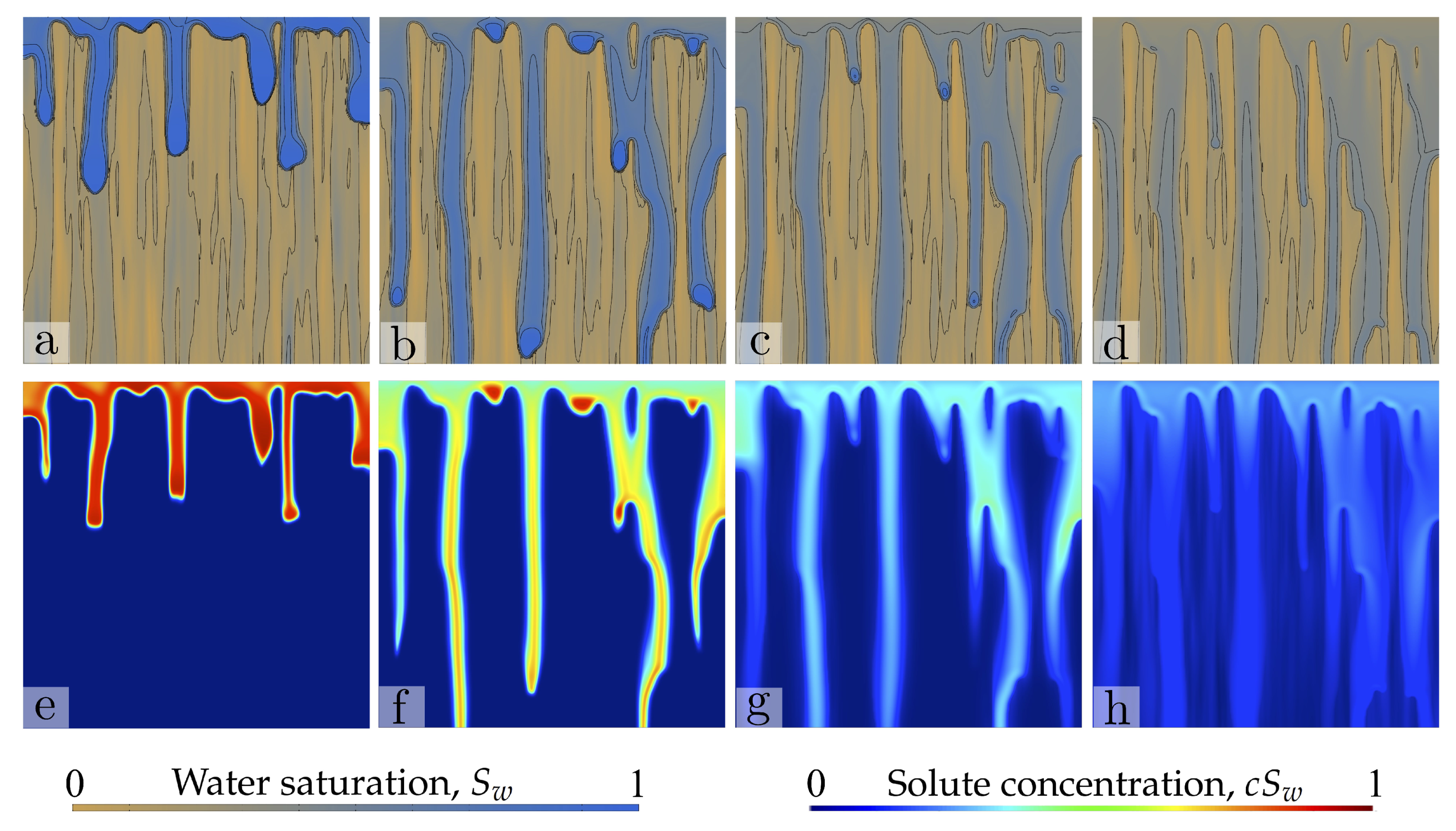
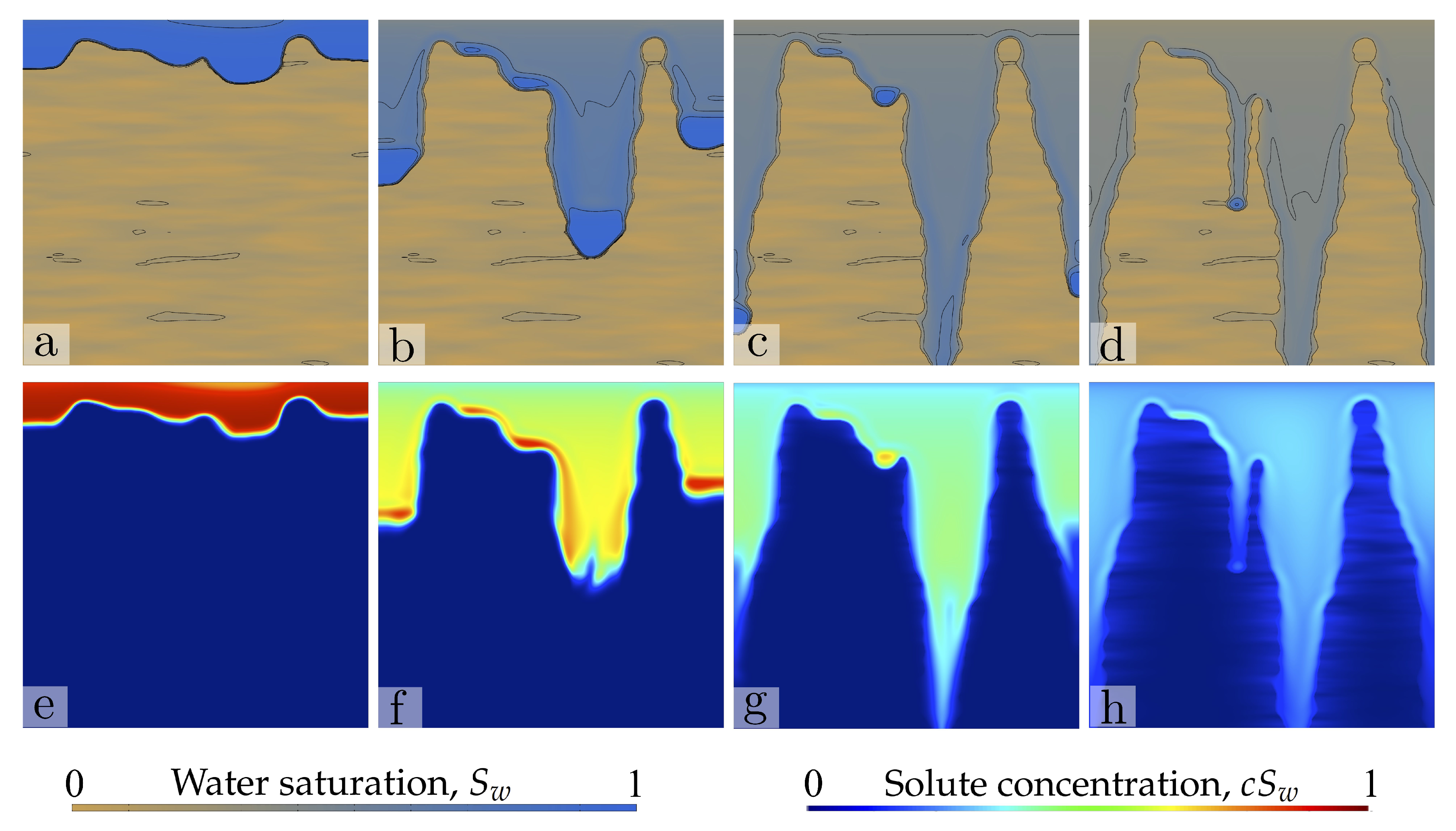
To illustrate the impact of initial water saturation on the patterns of solute transport and dilution, we simulate the transport of a solute deposited at the soil surface by a short water pulse, as described in Figure 5 and Section 4.1. We show sample 2D simulations with random initial saturation fields (Figure 8, Figure 9, Figure 10, Figure 11, Figure 12 and Figure 13). We consider cases with isotropic (Figure 8 and Figure 9) and anisotropic (Figure 10, Figure 11, Figure 12 and Figure 13) initial saturation fields, with various maximum initial saturations. We plot the maps of water saturation, , and solute concentration, , at times 100 s, 300 s, 1500 s and 15,000 s during water infiltration and redistribution.
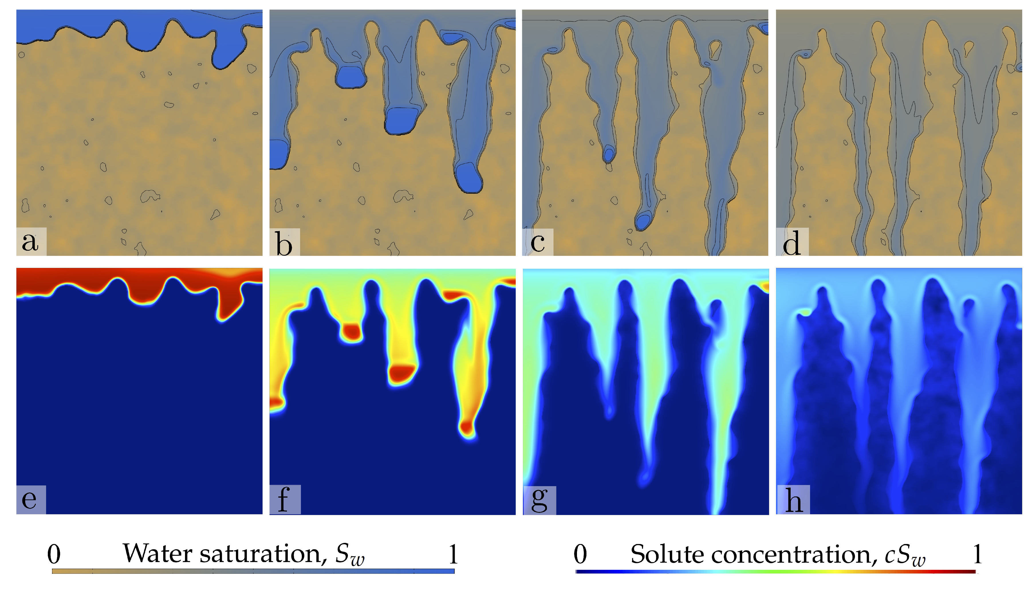
For the isotropic fields, we set a correlation length = = cm, and initial saturations = and (Figure 8 and Figure 9, respectively). For the anisotropic fields, we set correlation lengths = cm, = cm with initial saturations = and (Figure 10 and Figure 11, respectively), and = cm, = cm with initial saturations = and (Figure 12 and Figure 13, respectively). When using isotropic distributions of low initial water saturation (Figure 8) the infiltration patterns reduce to the standard result of straight, downward-moving fingers with typical finger sizes and spacing controlled by the internal hydrodynamic length scales, and . Solute transport is strongly focused through the fingers, with little dilution into the ambient water due to diffusion (Figure 8e–h). The randomly distributed pockets of large saturation that result from isotropic Gaussian fields (Figure 9) lead to intense finger meandering and merging, and the finger size is strongly influenced by the correlation length of initial water saturation. Finger meandering induces complex transport paths for the solute, enhancing solute dilution. Note that the overall flow structure retains its character of preferential flow due to the fingering instability.
Anisotropic distributions of initial water saturation resemble the initial state of a soil that has been subjected to cycles of infiltration before the simulated one (Figure 10, Figure 11, Figure 12 and Figure 13). Vertical correlation lengths that are much larger than the horizontal one (Figure 10 and Figure 11) induce fast vertical water and solute transport, as the presence of larger-conductivity wet regions strongly enhances the fingering instability. As the initial water content of the vertical channels increases, the lateral dilution of the solute induces a more homogeneous distribution of solute in the soil (Figure 11). Water pockets of lenticular shape (Figure 12 and Figure 13) thicken the finger size and induce lateral mixing of the solute. Lateral mixing becomes very efficient as the horizontal correlation length increases (Figure 13).
4.4. Analysis: Impact of the Spatial Structure of the iNitial Saturation Field on Water and Solute Transport
As a summary of the impact of the spatial structure of the initial saturation field on the patterns of water infiltration and solute transport, we plot the maps of water saturation and net solute concentration, at the same time, s, for several initial saturation fields (Figure 14 and Figure 15).
Firstly, we explore the impact of anisotropy (Figure 14), by comparing simulations with the same maximum initial saturation = , and three pairs of correlation length, = cm and = cm, = cm and = cm, and (Figure 15c) = cm and = cm. The flow pattern induced by the initial soil moisture distribution is important, as flow complexity (finger meandering and merging) helps solute mixing and dilution into the resident fresh water. The isotropic initial distribution (Figure 14a) leads to a more complex flow path behavior, due to finger reconnections driven by the pockets of higher water saturation. In contrast the vertically oriented initial saturation fields (Figure 14b) leads to focused flow along the pre-wet regions, thus reducing dilution of the infiltrating solute into the resident fresh water. Horizontal layering increases the characteristic finger size, allowing for lateral diffusion of the solute for large diffusivity/dispersivity (Figure 14c).
Secondly, we illustrate the impact of maximum saturation, by comparing simulations with the same correlation lengths, = cm and = cm, and four maximum initial saturations, = , = , = , and = , all of them at time t = 1500 s (Figure 15). When the initial saturation is low, the solute remains encapsulated by the water fingers, and dilution is limited to lateral diffusion/dispersion away from the finger cores (Figure 15a). Dilution is greatly enhanced by increasing initial saturation, which promotes both flow complexity and lateral diffusion (Figure 15b–d).
4.5. Analysis: Impact of the Solute Diffusivity/Dispersivity on the Effective Solute Dilution
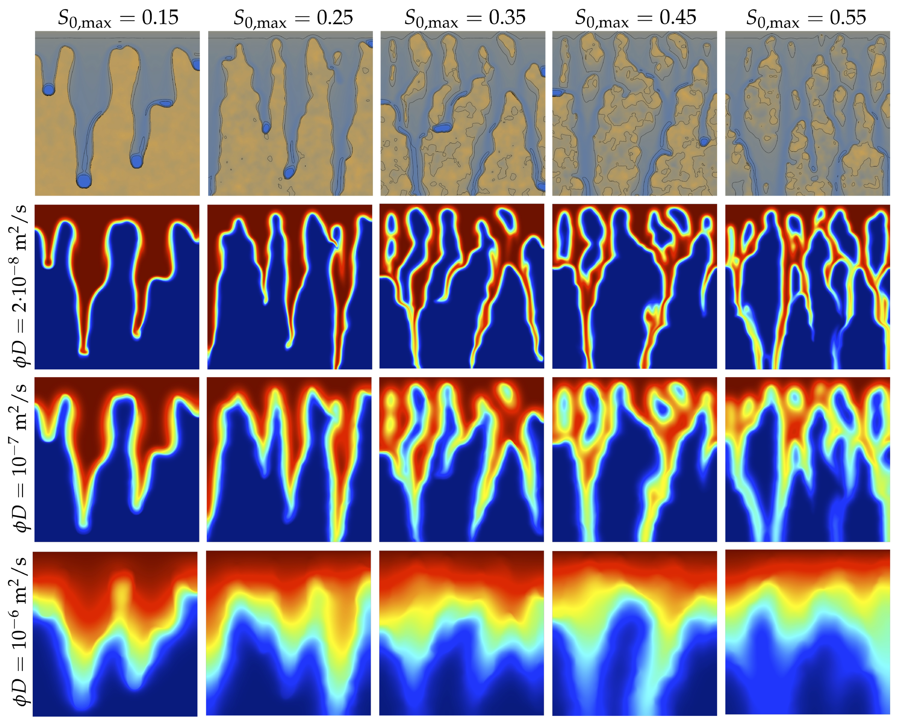
The dilution of the infiltrating solute is controlled by the preferential water flow, and by the effective diffusivity/dispersivity of solute. The former controls the overall water flow paths, while the latter determines the diffusion and dilution of solute into the ambient soil water. To elucidate the impact of effective diffusivity, we show the snapshot of water saturation and solute concentration in the pore water, c, at time 1500 s, for five different isotropic initial saturation fields (Figure 16). The maximum saturations are = , , , , (distributed along columns), and we consider three solute diffusivities/dispersivities, = 2· m/s, = m/s, and = m/s (along rows). Lower diffusivities lead to focusing of the solute transport along the preferential paths created by the infiltrating water fingers, with little dilution into the ambient freshwater.
4.6. Analysis: Solute Fluxes and Overall Statistics of the Concentration and Saturation Fields
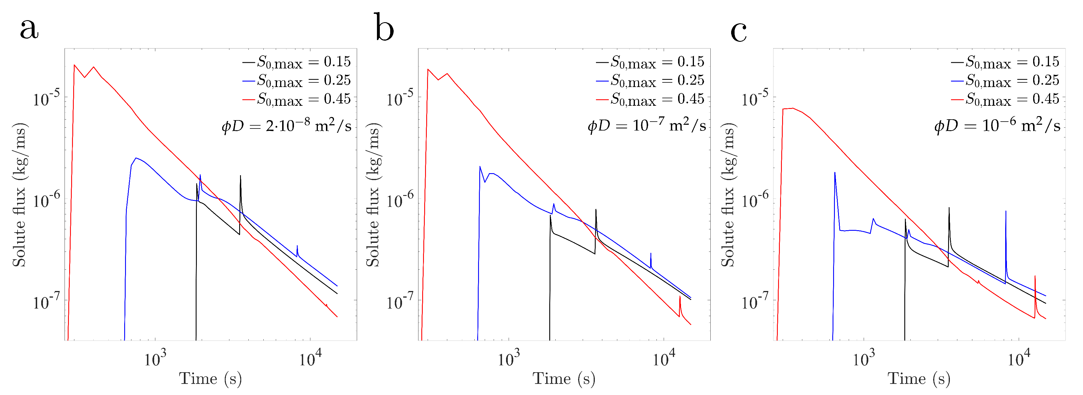
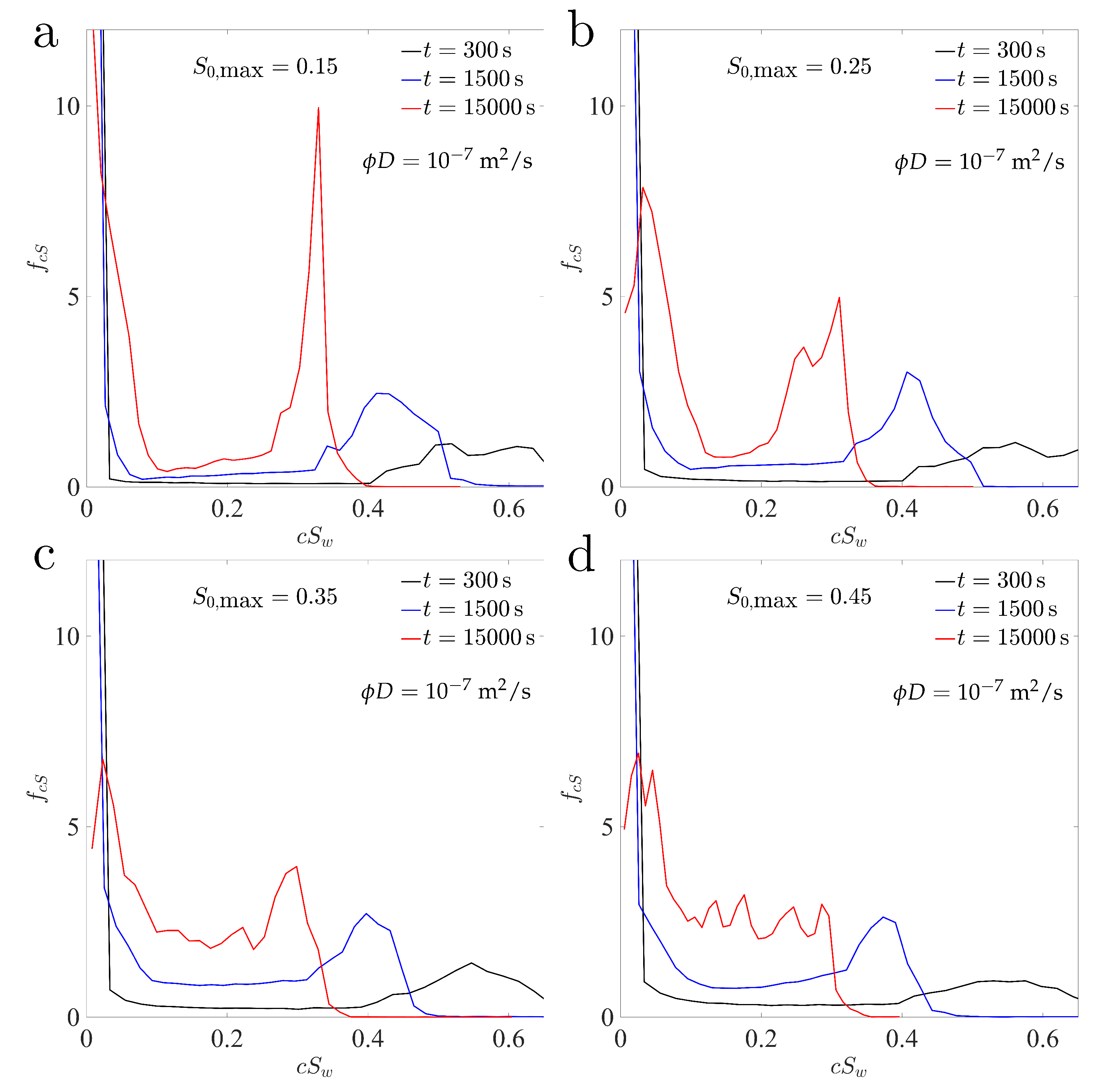
The integrated solute fluxes at the outlet (bottom of the domain) are consistent with the observed patterns of preferential flow and transport (Figure 17). We plot the evolution of solute flux for isotropic initial saturation field, = = cm, and three maximum saturations = , for serveral values of the effective diffusivity = 2· m/s, = m/s, and = m/s (Figure 17a–c, respectively). Larger initial saturations lead to earlier breakthrough of water and solute. Larger diffusivities lead to more intense dilution, which tends to delay the arrival of solute (slightly smaller fluxes at early times for the same initial saturation). The dilution effect is well-characterized by the evolution of the probability density function (pdf) of net concentration, (Figure 18 and Figure 19).
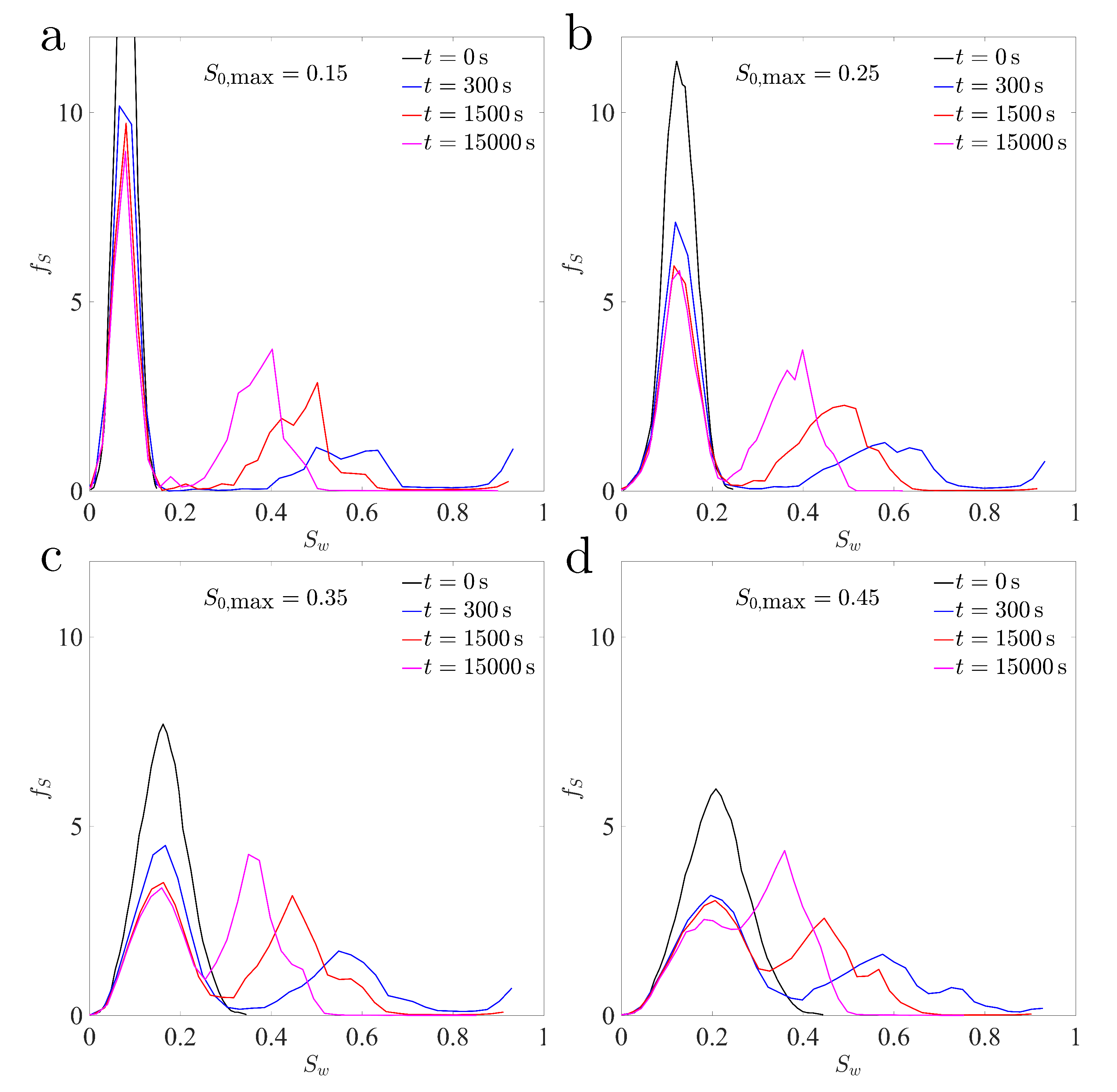
We study the evolution of the pdfs for isotropic (Figure 18), as well as anisotropic initial saturation fields (Figure 19). The pdfs appears bimodal in many cases, marking the concentrations in the fresh water and infiltrating water. Shifting of the second peak larger than zero concentration signals dilution of the infiltrating solute into the ambient water. In Figure 18c,d, the more continuous shape of the red solid curve suggests better mixing into the ambient water. It is interesting that the water saturation pdfs are different from the solute concentration one, indicating that dilution may reduce the correlations between soil moisture and solute concetration. The correlation between wet areas and zones with nonzero solute concentration is very high for relatively dry media (small value of the maximum initial saturation, Figure 19a,b), but the correlation decreases significantly for larger initial saturations (Figure 19c,d).
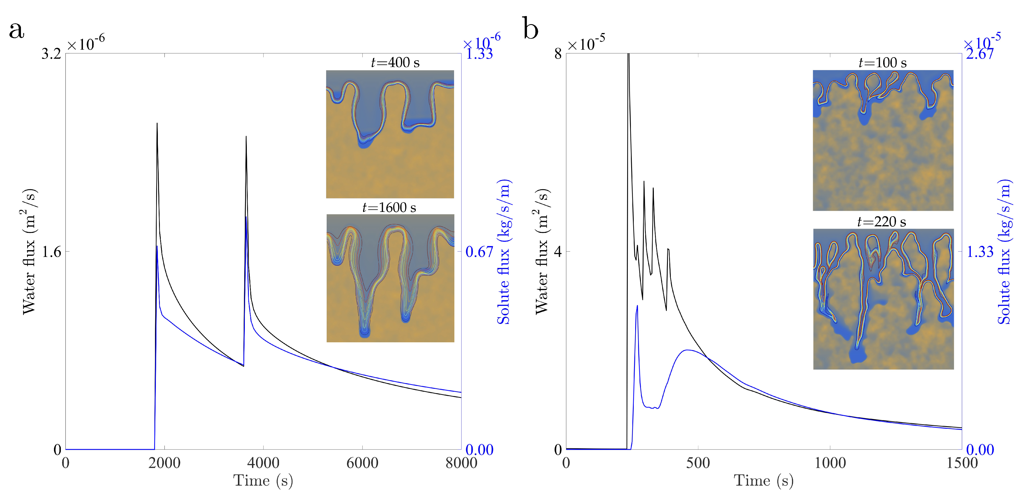
Finally, the delay in solute breakthrough due to the smaller speed of the solute front compared with the water front, is illustrated in Figure 20. For infiltration and transport into relatively dry soil (Figure 20a), the arrival of the infiltrating water and solute fronts is essentially simulataneous. The sharp water and solute peaks are due to the arrival of independent fingers. The strong peaks reveal the onset of saturation overshoots at the finger tips, which also lead to solute concentration overshoot, as in the 1D infiltration cases. When the initial water saturation increases (Figure 20b), there is a delay between the arrival of the water and solute fronts, in accordance with the 1D simulations. Note that the lag in solute concentration is due to mixing and dilution along the preferential flow paths, rather than to lateral mixing with the resident water. This behavior may be important in terms of estimating reactions, which seem to remain focused along fast flow paths, even in the case of soils that are already wet.
4.7. Solute Transport in Stable and Unstable Infiltration Fronts
To illistrate the impact of fingering instabilities on the patterns of solute transport during infiltration, we compare the results of our second-gradient model, which captures fingering instabilities, with those using Richards’ equation. The Richards equation corresponds to setting = 0 in Equations (4)–(8). As in previous sections, we simulate an infiltration pulse lasting 180 s, and study the redistribution of water and solute through the soil. We consider two random initial soil moisture fields, with the same spatial correlation lengths, = = cm, and two maximum saturations = (Figure 21 and Figure 22) and = (Figure 23 and Figure 24). We consider an effective diffusivity = m/s. The other model parameters are those listed in Table 1.
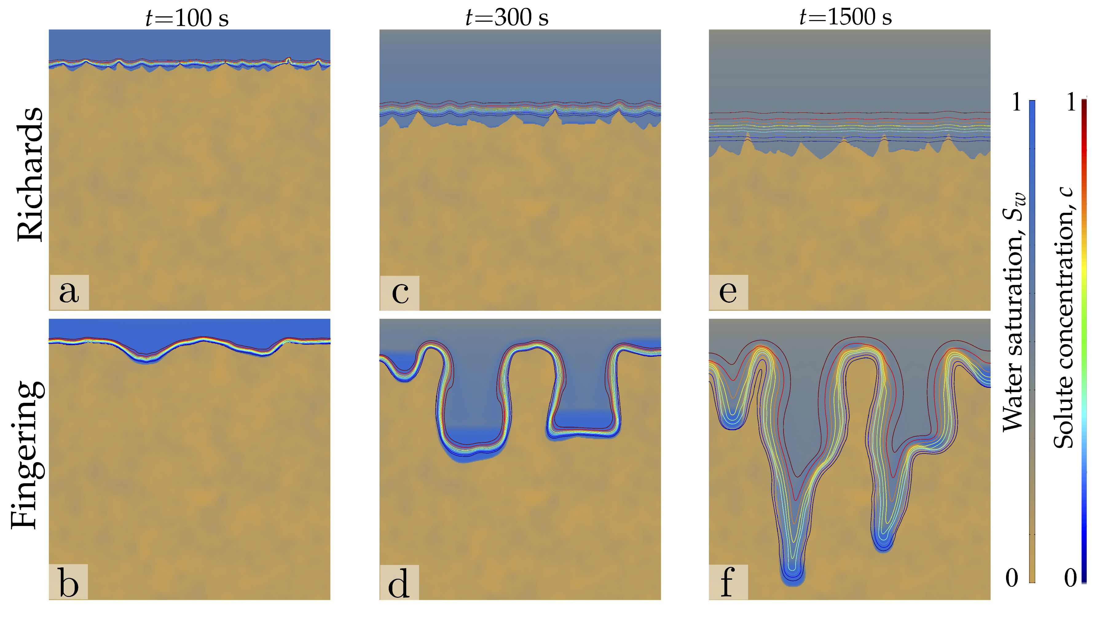
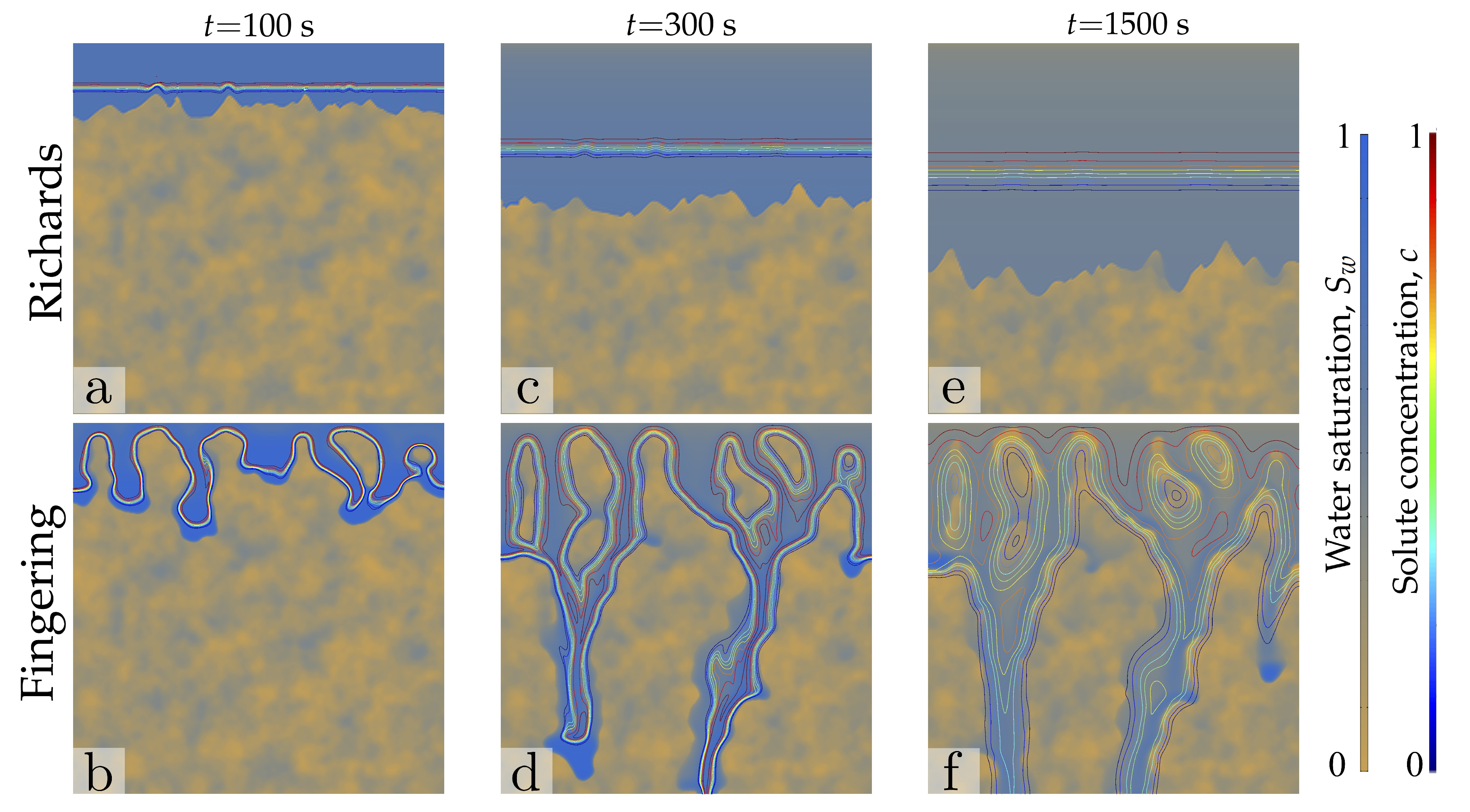
For the Richards equation, the infiltration front is stable for the two considered initial saturation fields (Figure 21a,c,e and Figure 23a,c,e). As predicted by the analytical result of Section 3.2, the solute and water fronts advance with similar speed for the low initial saturation case (Figure 21a,c,e), while the water front is significatly faster for the large initial saturation field (Figure 23a,c,e). In contrast, preferential flow due to fingering (Figure 21b,d,f and Figure 23b,d,f) leads to funneling of the solute into the fingers, and to early breakthrough of water and solute.
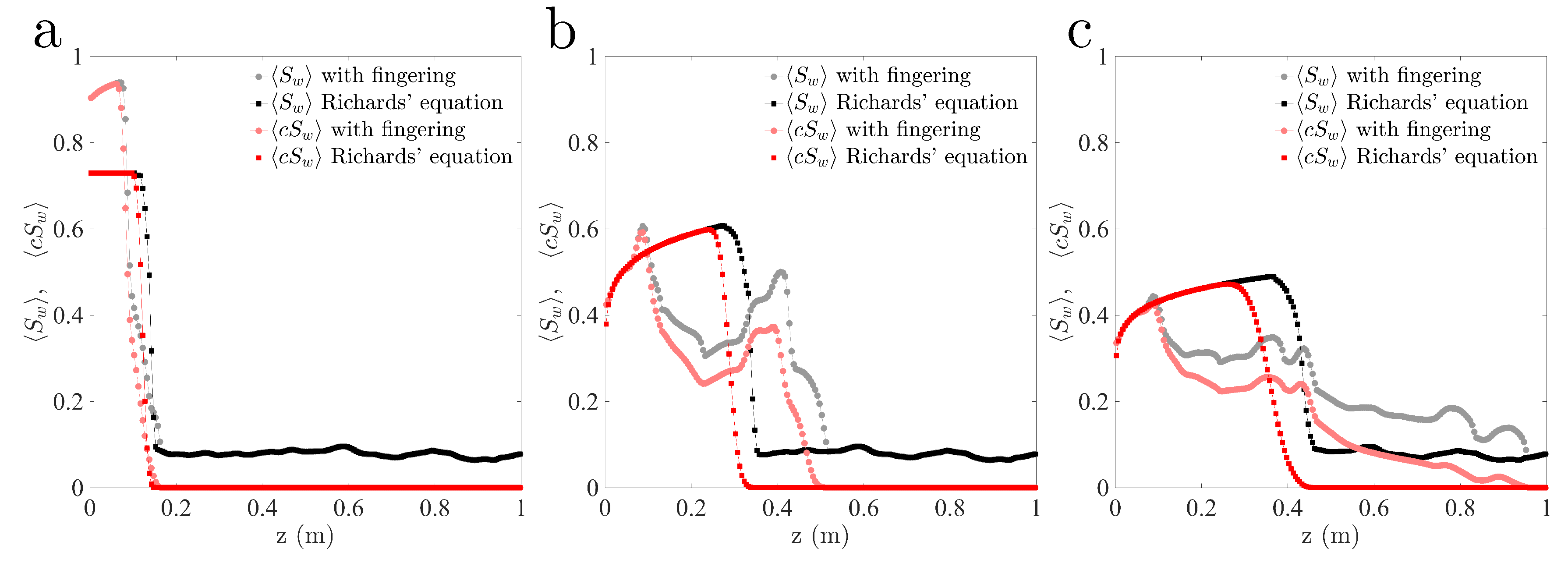
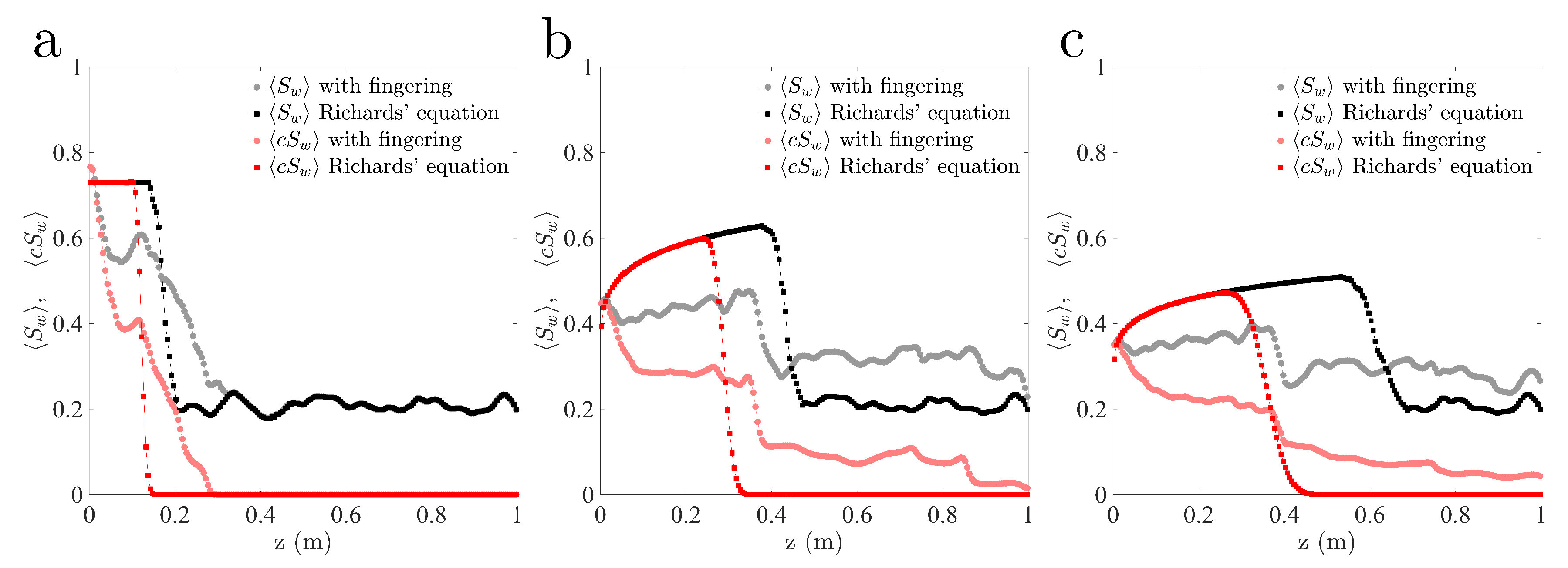
For these simulations using the Richards equation and the present second-gradient model, we also plot the x-averaged vertical profiles of water saturation and solute concentration, and (Figure 22 and Figure 24), at the same time levels as the snapshots shown in Figure 21 and Figure 23. The simulations using the Richards equation are quasi-1D, in the sense that compact infiltration fronts leads to water saturations and concentrations through the soil column that could be predicted from 1D simulations. The profiles of fingered infiltration are markedly different, with earlier breakthrough and strong dispersion, which arise from inherently two-dimensional flow structures.
5. Conclusions
In this paper, we have studied preferential solute transport in the vadose zone, by simulating coupled unsaturated flow and advection–diffusion of a passive tracer. The patterns of preferential flow and solute transport and dilution into the ambient preexisting soil water are controlled by the spatial patterns of the distribution of initial pore water. We control the latter by generating random correlated fields with multi-Gaussian statistics. The flow model is based on a thermodynamic description that extends Richards’ equation to allow for unstable wetting fronts and the formation of gravity fingers during infiltration. The initial water saturation fields with spatial correlation are characterized by a maximum saturation (the minimum saturation is held at 0.01), and the correlation lengths. With these randomly correlated fields we aim at resembling the initial state of the soil after several cycles of infiltration and redistribution prior to the simulated infiltration pulse. We consider isotropic random fields, with equal horizontal and vertical correlation lengths, as well as anisotropic fields, with correlation structures that either favor vertical correlation (resembling a pattern of previous fingered flow) or horizontal (resembling a pattern of previous redistribution leading to water lenses). Unstable infiltration, leading to fingering, and the presence of water pockets in the soil, determines the flow and solute mixing patterns during infiltration and redistribution of the infiltrating saltwater.
An important factor in solute transport in unsaturated flow through soil with some initial water saturation is that the water and solute fronts may travel at different speeds. We explain and characterize this phenomenon in 1D constant-rate infiltration and solute transport (Section 3), and then verify that it is also a property of multidimensional transport (Section 4.6).
Our main findings and conclusions are as follows:
- To the best of our knowledge, these are the first numerical simulations of solute transport during unstable infiltration into soil. We show that the patterns of water flow and solute transport arising from unstable infiltration are very different from those obtained using Richards’ equation, which predicts compact, stable front of water saturation and solute concentration.
- The initial water content and its spatial distribution play a key role in the patterns of water infiltration and solute transport in unsaturated coarse soil. The structure of initial freshwater saturation controls solute transport through two mechanisms: (1) the interplay between the fingering instability and the increased conductivity at the wet patches; (2) the lateral dilution of solute into the ambient water. The extent to which the former mechanism controls transport is related to the anisotropy of the initial water saturation field and to the maximum saturations at the water pockets. Isotropic distributions of low initial water saturation lead to the classical straight, downward-moving fingers, with finger sizes and spacing controlled by the internal hydrodynamic length scales. Isotropic fields with large saturation lead to complex infiltration patterns, with finger meandering and efficient solute dilution into the ambient water. Anisotropic fields with preferentially vertical correlation, combined with the fingering instability, promote focused transport and reduce mixing to the extent of lateral dilution due to solute diffusion/dispersion. Water pockets of lenticular shape thicken the finger size and induce lateral mixing of the solute. Lateral mixing becomes very efficient as the horizontal correlation length increases.
- The effective diffusivity/dispersivity of solute is particularly important for solute dilution in dry soils, or in those where the initial water saturation field induces flow focusing (vertical correlation). When the initial saturation field leads to complex infiltration patterns (the presence of water lenses or isotropic fields with large saturation), the flow field is complex and enhances mixing, leading to more efficient dilution.
- The integrated solute fluxes at the outlet (bottom of the domain) are consistent with the one-dimensional prediction of a delayed arrival of the solute when the soil is initially wet.
Our simulations show that hydrodynamic instabilities are essential to understand the travel times of solutes and pollutants, as well as their mass fluxes towards groundwater bodies. The flow patterns resulting from the interplay between fingering instabilities and initial soil moisture suggest that early breakthrough and tailing of water and solute fluxes should be expected for infiltration into sandy soil, with little dilution of the solute with the resident water, at least for mildly wet soils. The mixing and transport behavior may be amenable to modeling using non-Fickian theories of transport, including mobile–immobile approaches, Continuous Time Random Walk (CTRW) descriptions, or transport models based on the fractional advection–dispersion equation (fADE). This work offors insights into the behavior of infiltration in natural systems, including the design and optimization of irrigation systems, the transport of contaminants through the vadose zone and into groundwater bodies, and better understanding on natural markers such as radionucleids, mixing and reactions in heterogeneous soils at the Darcy and field scales.
Author Contributions
Investigation L.C.-F., M.J.S.-N., X.F. and R.J. All authors have read and agreed to the published version of the manuscript.
Funding
Funding for this research was provided by Spanish Ministry of Economy and Competitiveness under grant CTM2014-54312-P (to L.C.-F.), by the Abdul Latif Jameel World Water and Food Security Lab (J-WAFS) at MIT (to R.J.), by the MIT International Science and Technology Initiatives (MISTI), through a Seed Fund grant (to R.J. and L.C.-F.), and by the Miller Fellowship for Basic Research in Science (to X.F.).
Conflicts of Interest
The authors declare no conflict of interest. The funders had no role in the design of the study; in the collection, analyses, or interpretation of data; in the writing of the manuscript, or in the decision to publish the results.
References
- Nielsen, D.R.; van Genuchten, M.T.; Biggar, J.W. Water Flow and Solute Transport Processes in the Unsaturated Zone. Water Resour. Res. 1986, 22, 89S–108S. [Google Scholar] [CrossRef]
- Candela, L.; Caballero, J.; Ronen, D. Glyphosate transport through weathered granite soils under irrigated and non-irrigated conditions—Barcelona, Spain. Sci. Total Environ. 2010, 408, 2509–2516. [Google Scholar] [CrossRef]
- Botros, F.E.; Onsoy, Y.S.; Ginn, T.R.; Harter, T. Richards Equation-Based Modeling to Estimate Flow and Nitrate Transport in a Deep Alluvial Vadose Zone. Vadose Zone J. 2012, 11, 4–20. [Google Scholar] [CrossRef] [Green Version]
- Silber, A.; Israeli, Y.; Elingold, I.; Levi, M.; Levkovitch, I.; Russo, D.; Assouline, S. Irrigation with desalinated water: A step toward increasing water saving and crop yields. Water Resour. Res. 2015, 51, 450–464. [Google Scholar] [CrossRef]
- Valdes-Abellan, J.; Jiménez-Martínez, J.; Candela, L.; Jacques, D.; Kohfahl, C.; Tamoh, K. Reactive transport modelling to infer changes in soil hydraulic properties induced by non-conventional water irrigation. J. Hydrol. 2017, 549, 114–124. [Google Scholar] [CrossRef] [Green Version]
- Zhuang, J.; Tyner, J.S.; Perfect, E. Colloid transport and remobilization in porous media during infiltration and drainage. J. Hydrol. 2009, 377, 112–117. [Google Scholar] [CrossRef]
- Torkzaban, S.; Hassanizadeh, S.; Schijven, J.F.; de Bruin, A.M.; de Roda Husman, A.M. Virus transport in saturated and unsaturated sand columns. Vadose Zone J. 2006, 5, 877–885. [Google Scholar] [CrossRef] [Green Version]
- Zhang, Q.; Hassanizadeh, S.M.; Raoof, A.; van Genuchten, M.T.; Roels, S.M. Modeling Virus Transport and Remobilization during Transient Partially Saturated Flow. Vadose Zone J. 2012, 11. [Google Scholar] [CrossRef]
- Jiménez-Martínez, J.; de Anna, P.; Tabuteau, H.; Turuban, R.; Borgne, T.L.; Méheust, Y. Pore-scale mechanisms for the enhancement of mixing in unsaturated porous media and implications for chemical reactions. Geophys. Res. Lett. 2015, 42, 5316–5324. [Google Scholar] [CrossRef] [Green Version]
- Jiménez-Martínez, J.; Borgne, T.L.; Tabuteau, H.; Méheust, Y. Impact of saturation on dispersion and mixing in porous media: Photobleaching pulse injection experiments and shear-enhanced mixing model. Water Resour. Res. 2017, 53, 1457–1472. [Google Scholar] [CrossRef] [Green Version]
- Jiménez-Martínez, J.; Porter, M.L.; Hyman, J.D.; Carey, J.W.; Viswanathan, H.S. Mixing in a three-phase system: Enhanced production of oil-wet reservoirs by CO2 injection. Geophys. Res. Lett. 2016, 43, 196–205. [Google Scholar] [CrossRef]
- Russo, D.; Zaidel, J.; Laufer, A. Numerical analysis of flow and transport in a three–dimensional partially saturated heterogeneous soil. Water Resour. Res. 1998, 34, 1451–1468. [Google Scholar] [CrossRef]
- Starr, J.L.; Parlange, J.Y.; Frink, C.R. Water and chloride movement through a layered field soil. Soil Sci. Soc. Am. J. 1994, 50, 1384–1390. [Google Scholar] [CrossRef]
- Steenhuis, T.S.; Parlange, J.Y.; Andreini, M.S. A Numerical Model for Preferential Solute Movement in Structured Soils. Geoderma 1990, 46, 193–208. [Google Scholar] [CrossRef]
- Snow, V.O.; Clothier, B.E.; Scotter, D.R.; White, R.E. Solute transport in a layered field soil: Experiments and modelling using the convection-dispersion approach. J. Contaminant Hydrol. 1994, 16, 339–358. [Google Scholar] [CrossRef]
- Koestel, J.; Larsbo, M. Imaging and quantification of preferential solute transport in soil macropores. Water Resour. Res. 2014, 50, 4357–4378. [Google Scholar] [CrossRef]
- Jiménez-Martínez, J.; Tamoh, K.; Candela, L.; Elorza, F.; Hunkeler, D. Multiphase Transport of Tritium in Unsaturated Porous Media—Bare and Vegetated Soils. Math. Geosci. 2012, 44, 187–208. [Google Scholar] [CrossRef] [Green Version]
- Russo, D. Alternating irrigation water quality as a method to control solute concentrations and mass fluxes below irrigated fields: A numerical study. Water Resour. Res. 2016, 52, 3440–3456. [Google Scholar] [CrossRef]
- Russo, D. Effect of pulse release date and soil characteristics on solute transport in a combined vadose zone-groundwater flow system: Insights from numerical simulations. Water Resour. Res. 2011, 47, W05532. [Google Scholar] [CrossRef] [Green Version]
- Richards, L.A. Capillary conduction of liquids through porous mediums. Physics 1931, 1, 318–333. [Google Scholar] [CrossRef]
- Horton, R.E. The role of infiltration in the hydrologic cycle. Trans. Am. Geophys. Union 1933, 14, 446–460. [Google Scholar] [CrossRef]
- Philip, J.R. The theory of infiltration 1. The infiltration equation and its solution. Soil Sci. 1957, 83, 345–357. [Google Scholar] [CrossRef]
- Philip, J.R. Theory of infiltration. In Advances in Hydroscience; Chow, V.T., Ed.; Academic Press: New York, NY, USA, 1969; pp. 215–296. [Google Scholar]
- Jiménez-Martínez, J.; Skaggs, T.; van Genuchten, M.; Candela, L. A root zone modelling approach to estimating groundwater recharge from irrigated areas. J. Hydrol. 2009, 367, 138–149. [Google Scholar] [CrossRef]
- Jiménez-Martínez, J.; Candela, L.; Molinero, J.; Tamoh, K. Groundwater recharge in irrigated semi-arid areas: quantitative hydrological modelling and sensitivity analysis. Hydrogeol. J. 2010, 18, 1811–1824. [Google Scholar] [CrossRef]
- Šimůnek, J.; Jarvis, N.J.; van Genuchten, M.T.; Gärdenäs, A. Review and comparison of models for describing non-equilibrium and preferential flow and transport in the vadose zone. J. Hydrol. 2003, 272, 14–35. [Google Scholar] [CrossRef]
- Russo, D.; Laufer, A.; Gerstl, Z.; Ronen, D.; Weisbrod, N.; Zentner, E. On the mechanism of field-scale solute transport: Insights from numerical simulations and field observations. Water Resour. Res. 2014, 50, 7484–7504. [Google Scholar] [CrossRef]
- Šimůnek, J.; van Genuchten, M.T. Modeling Nonequilibrium Flow and Transport Processes Using HYDRUS. Vadose Zone J. 2008, 7, 782–797. [Google Scholar] [CrossRef] [Green Version]
- Raoof, A.; Hassanizadeh, S.M.; Leijnse, A. Upscaling Transport of Adsorbing Solutes in Porous Media: Pore-Network Modeling. Vadose Zone J. 2010, 9, 624–636. [Google Scholar] [CrossRef]
- Raoof, A.; Hassanizadeh, S.M. Saturation-dependent solute dispersivity in porous media: Pore-scale processes. Water Resour. Res. 2013, 49, 1943–1951. [Google Scholar] [CrossRef]
- de Vries, E.T.; Raoof, A.; van Genuchten, M.T. Multiscale modelling of dual-porosity porous media; a computational pore-scale study for flow and solute transport. Adv. Water Resour. 2017, 105, 82–95. [Google Scholar] [CrossRef]
- Szymkiewicz, A.; Gumuła-Kawęcka, A.; Potrykus, D.; Jaworska-Szulc, B.; Pruszkowska-Caceres, M.; Gorczewska-Langner, W. Estimation of Conservative Contaminant Travel Time through Vadose Zone Based on Transient and Steady Flow Approaches. Water 2018, 10, 1417. [Google Scholar] [CrossRef] [Green Version]
- Hill, D.E.; Parlange, J.Y. Wetting front instability in layered soils. Soil Sci. Soc. Am. J. 1972, 36, 697–702. [Google Scholar] [CrossRef]
- Glass, R.J.; Parlange, J.Y.; Steenhuis, T.S. Wetting front instability, 2. Experimental determination of relationships between system parameters and two-dimensional unstable flow field behaviour in initially dry porous media. Water Resour. Res. 1989, 25, 1195–1207. [Google Scholar] [CrossRef]
- Ritsema, C.J.; Dekker, L.W.; Nieber, J.L.; Steenhuis, T.S. Modeling and field evidence of finger formation and finger recurrence in a water repellent sandy soil. Water Resour. Res. 1998, 34, 555–567. [Google Scholar] [CrossRef] [Green Version]
- DiCarlo, D.A. Stability of gravity-driven multiphase flow in porous media: 40 years of advancements. Water Resour. Res. 2013, 49, 4531–4544. [Google Scholar] [CrossRef]
- Xiong, Y. Flow of water in porous media with saturation overshoot: A review. J. Hydrol. 2014, 510, 353–362. [Google Scholar] [CrossRef]
- Glass, R.J.; Oosting, G.H.; Steenhuis, T.S. Preferential solute transport in layered homogeneous sands as a consequence of wetting front instability. J. Hydrol. 1989, 110, 87–105. [Google Scholar] [CrossRef]
- Muskat, M.; Meres, M.W. The flow of heterogeneous fluids through porous media. Physics 1936, 7, 346–363. [Google Scholar] [CrossRef]
- Muskat, M. Physical Principles of Oil Production; McGraw-Hill: New York, NY, USA, 1949. [Google Scholar]
- Bear, J. Dynamics of Fluids in Porous Media; Elsevier: New York, NY, USA, 1972. [Google Scholar]
- Cueto-Felgueroso, L.; Juanes, R. Nonlocal interface dynamics and pattern formation in gravity-driven unsaturated flow through porous media. Phys. Rev. Lett. 2008, 101, 244504. [Google Scholar] [CrossRef] [Green Version]
- Cueto-Felgueroso, L.; Juanes, R. A phase-field model of unsaturated flow. Water Resour. Res. 2009, 45, W10409. [Google Scholar] [CrossRef]
- Sciarra, G. Phase field modeling of partially saturated deformable porous media. J. Mech. Phys. Solids 2016, 94, 230–256. [Google Scholar] [CrossRef] [Green Version]
- Beljadid, A.; Cueto-Felgueroso, L.; Juanes, R. A continuum model of unstable infiltration in porous media endowed with an entropy function. Adv. Water Resour. 2019. in review. [Google Scholar]
- Leverett, M.C. Capillary behavior of porous solids. Petrol. Trans. AIME 1941, 142, 152–169. [Google Scholar] [CrossRef]
- Aavatsmark, I. Capillary energy and the entropy condition for the Buckley-Leverett equation. In Current Progress in Hyperbolic Systems: Riemann Problems and Computations; Contemporary Mathematics; Lindquist, W.B., Ed.; American Mathematical Society: Providence, RI, USA, 1989; Volume 100, pp. 21–25. [Google Scholar]
- Aavatsmark, I. Kapillarenergie als Entropiefunktion. Z. Angew. Math. Mech. 1989, 69, 319–327. [Google Scholar] [CrossRef]
- COMSOL. COMSOL Multiphysics Structural Mechanics Module User’s Guide v5.2a; Comsol: Stockholm, Sweden, 2016. [Google Scholar]
- Brooks, R.H.; Corey, A.T. Properties of porous media affecting fluid flow. J. Irrig. Drain. Div. Proc. Am. Soc. Civ. Eng. 1966, IR2, 61–88. [Google Scholar]
- van Genuchten, M.T. A closed-form equation for predicting the hydraulic conductivity of unsaturated soils. Soil Sci. Soc. Am. J. 1980, 44, 892–898. [Google Scholar] [CrossRef] [Green Version]
- Gelhar, L.W.; Axness, C.L. Three-Dimensional Stochastic Analysis of Macrodispersion in Aquifers. Water Resour. Res. 1983, 19, 161–180. [Google Scholar] [CrossRef]
Figure 1.
Schematic of 1D simulations of coupled unsaturated flow and transport in a soil column. (a) We simulate constant-rate infiltration into soil with initial freshwater saturation. The infiltrating water has a constant solute concentration. (b) The capillary pressure–saturation curve (Leverett’s J function) and relative permeability curves used in this study.

Figure 2.
Solute and water front speeds in constant-rate infiltration into soil with initial fresh water saturation (Equations (29) and (30)). The water front speed is given by the slope of the secant line joining the relative mobilities of the initial and inflow saturations (blue and red dots, respectively), while the solute front speed is given by the slope of the secant line from zero to the inflow relative mobility.

Figure 3.
One-dimensional profiles of solute transport during infiltration. For the same constant flux ratio = , we show profiles for three initial saturations, , at time t = 30 s. (a) For = , (b) = , and (c) = . Black (resp. blue) vertical dotted lines correspond to the water (solute) front positions predicted by Equations (29) and (30). Red (resp. blue) dots indicate the left-state (resp. right-state) water saturations, (resp. ) used to illustrate the different front velocities in Figure 2.

Figure 4.
One-dimensional profiles of solute transport during infiltration. For the same constant flux ratio = , we show profiles for three initial saturations, , at time t = 520 s. (a) For = , (b) = , and (c) = . Black (resp. blue) vertical dotted lines correspond to the water (solute) front positions predicted by Equations (29) and (30).

Figure 5.
Two-dimensional problem set-up. (a) We simulate coupled unsaturated flow and solute transport during infiltration into soil with an initial distribution of fresh water. We simulate a pulse infiltration of water with a given solute concentration, as constant water flux at the top boundary for a short time period of 180 s. (b,c) We study the impact of initial soil moisture distribution on the patterns of water flow and transport, and on the solute flux at the bottom of the domain. We couple unsaturated flow with he advection–dispersion equation, to compute the evolution of (b) water saturation (the fraction of pore volume occupied by water) and (c) solute concentration.

Figure 6.
Characteristics of isotropic initial saturation fields. (a–d) Maps of initial saturation, which are random isotropic fields characterized by the maximum initial saturation, , and correlation lengths, and . The minimum initial saturation is the same in all cases, . Here we show sample fields with = = cm, and (a) = , (b) = , (c) = , (d) = . (e) Probability density functions of initial saturation for the saturation fields shown in panels (a–d).

Figure 7.
Characteristics of anisotropic initial saturation fields. (a–c) Maps of initial saturation, which are random fields characterized by the maximum initial saturation, , and correlation lengths, and . The minimum initial saturation is the same in all cases, = . Here we show sample fields with = , and correlation lengths (a) = = cm, (b) = cm, = cm, (c) = cm, = cm. (d) Probability density functions of initial saturation for the saturation fields shown in panels (a–c).

Figure 8.
Sample 2D simulations of unstable infiltration and solute transport in soil with random initial saturation. We simulate the transport of a solute deposited at the soil surface by a short water pulse. We consider constant solute concentration at the top ( = 1 kg/m). The infiltration pulse is modeled as a constant water flux along the top boundary during a period of 180 s. The initial saturation field is isotropic, with maximum saturation = , and correlation lengths = = cm. (a–d) Maps of water saturation, , at times 100 s, 300 s, 1500 s and 15,000 s. (e–h) Maps of net solute concentration, , at the same time levels.

Figure 9.
Sample 2D simulations of unstable infiltration and solute transport in soil with random initial saturation. We simulate the transport of a solute deposited at the soil surface by a short water pulse. We consider constant solute concentration at the top ( = 1 kg/m). The infiltration pulse is modeled as a constant water flux along the top boundary during a period of 180 s. The initial saturation field is isotropic, with maximum saturation = , and correlation lengths cm. (a–d) Maps of water saturation, , at times 100 s, 300 s, 1500 s and 15,000 s. (e–h) Maps of net solute concentration, , at the same time levels.

Figure 10.
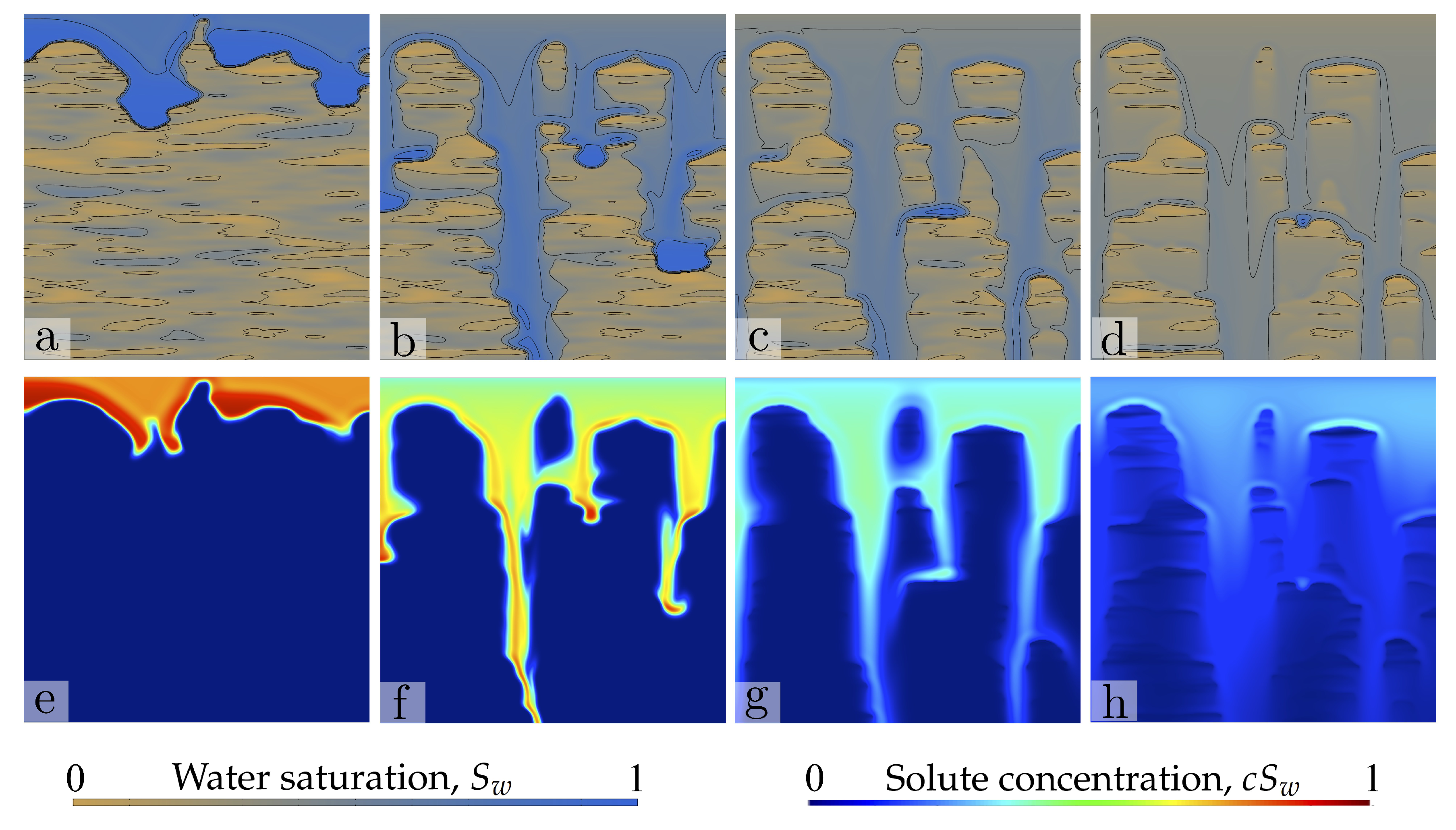
Sample 2D simulations of unstable infiltration and solute transport in soil with random initial saturation. We simulate the transport of a solute deposited at the soil surface by a short water pulse. We consider constant solute concentration at the top ( = 1 kg/m). The infiltration pulse is modeled as a constant water flux along the top boundary during a period of 180 s. The initial saturation field is anisotropic, with maximum saturation = , and correlation lengths = cm, cm. (a–d) Maps of water saturation, , at times 100 s, 300 s, 1500 s and 15,000 s. (e–h) Maps of net solute concentration, , at the same time levels.
Figure 10.
Sample 2D simulations of unstable infiltration and solute transport in soil with random initial saturation. We simulate the transport of a solute deposited at the soil surface by a short water pulse. We consider constant solute concentration at the top ( = 1 kg/m). The infiltration pulse is modeled as a constant water flux along the top boundary during a period of 180 s. The initial saturation field is anisotropic, with maximum saturation = , and correlation lengths = cm, cm. (a–d) Maps of water saturation, , at times 100 s, 300 s, 1500 s and 15,000 s. (e–h) Maps of net solute concentration, , at the same time levels.

Figure 11.
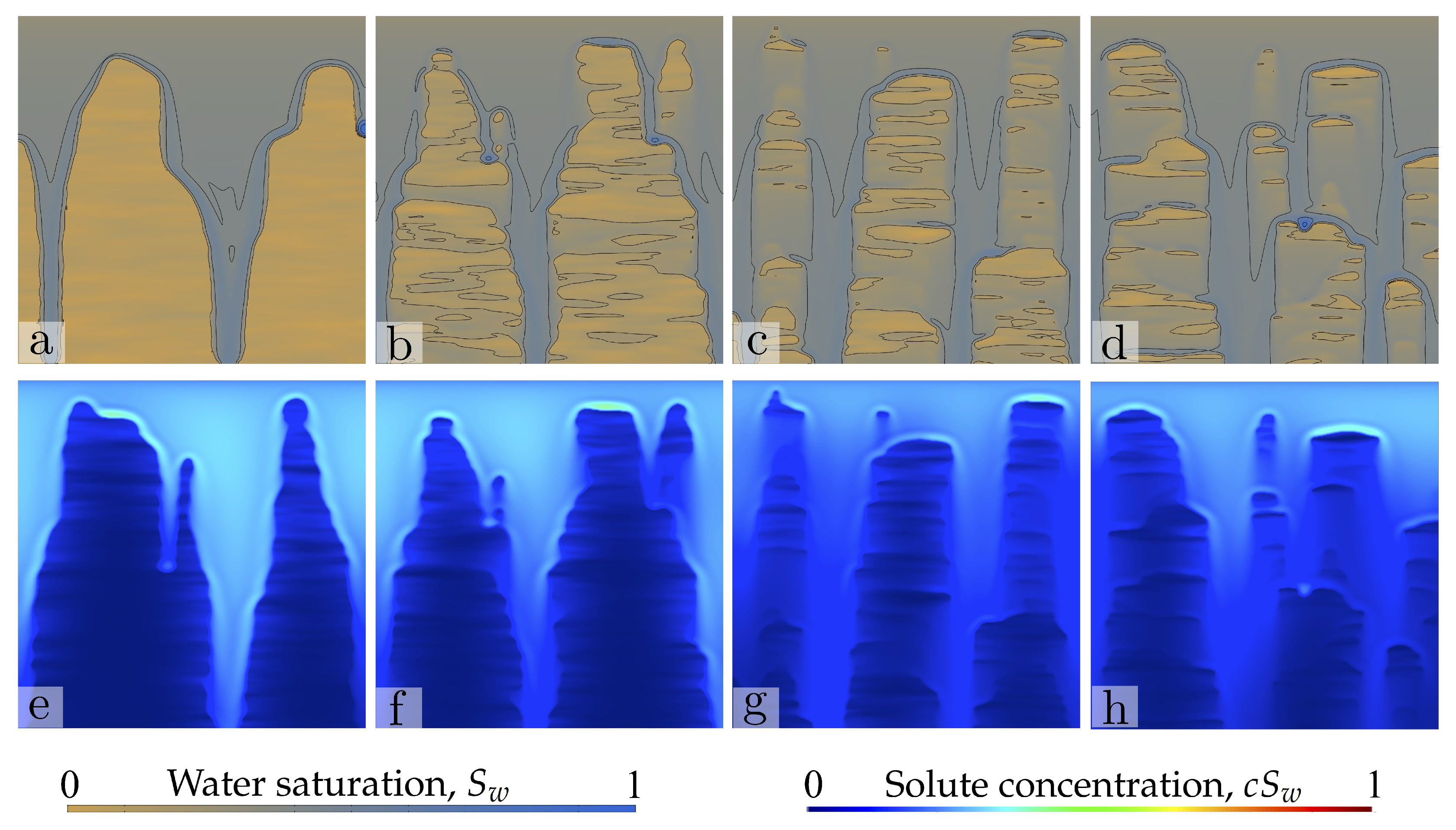
Sample 2D simulations of unstable infiltration and solute transport in soil with random initial saturation. We simulate the transport of a solute deposited at the soil surface by a short water pulse. We consider constant solute concentration at the top ( = 1 kg/m). The infiltration pulse is modeled as a constant water flux along the top boundary during a period of 180 s. The initial saturation field is anisotropic, with maximum saturation = , and correlation lengths = cm, = cm. (a–d) Maps of water saturation, , at times 100 s, 300 s, 1500 s and 15,000 s. (e–h) Maps of net solute concentration, , at the same time levels.
Figure 11.
Sample 2D simulations of unstable infiltration and solute transport in soil with random initial saturation. We simulate the transport of a solute deposited at the soil surface by a short water pulse. We consider constant solute concentration at the top ( = 1 kg/m). The infiltration pulse is modeled as a constant water flux along the top boundary during a period of 180 s. The initial saturation field is anisotropic, with maximum saturation = , and correlation lengths = cm, = cm. (a–d) Maps of water saturation, , at times 100 s, 300 s, 1500 s and 15,000 s. (e–h) Maps of net solute concentration, , at the same time levels.

Figure 12.
Sample 2D simulations of unstable infiltration and solute transport in soil with random initial saturation. We simulate the transport of a solute deposited at the soil surface by a short water pulse. We consider constant solute concentration at the top ( = 1 kg/m). The infiltration pulse is modeled as a constant water flux along the top boundary during a period of 180 s. The initial saturation field is anisotropic, with maximum saturation = , and correlation lengths = cm, = cm. (a–d) Maps of water saturation, , at times 100 s, 300 s, 1500 s and 15,000 s. (e–h) Maps of net solute concentration, , at the same time levels.

Figure 13.
Sample 2D simulations of unstable infiltration and solute transport in soil with random initial saturation. We simulate the transport of a solute deposited at the soil surface by a short water pulse. We consider constant solute concentration at the top ( = 1 kg/m). The infiltration pulse is modeled as a constant water flux along the top boundary during a period of 180 s. The initial saturation field is anisotropic, with maximum saturation = , and correlation lengths = cm, = cm. (a–d) Maps of water saturation, , at times 100 s, 300 s, 1500 s and 15,000 s. (e–h) Maps of net solute concentration, , at the same time levels.

Figure 14.
Influence of the spatial structure of the initial saturation field on solute transport in unstable infiltration. We simulate the transport of a solute deposited at the soil surface by a short water pulse. We consider constant solute concentration at the top ( = 1 kg/m). The infiltration pulse is modeled as a constant water flux along the top boundary during a period of 180 s. The initial saturation field is anisotropic, with maximum saturation = . (a–c) Maps of water saturation, , at time 1500 s for an initial saturation field with correlation lengths (a) = cm, = cm, (b) = cm, = cm, (c) = cm, = cm. (d–f) Maps of net solute concentration, , at the same time.

Figure 15.
Influence of the spatial structure of the initial saturation field on solute transport in unstable infiltration. We simulate the transport of a solute deposited at the soil surface by a short water pulse. We consider constant solute concentration at the top ( = 1 kg/m). The infiltration pulse is modeled as a constant water flux along the top boundary during a period of 180 s. The initial saturation field is anisotropic, with correlation length = cm, = , and several values of the maximum saturation. (a–d) Maps of water saturation, , at time 1500 s for an initial saturation field with maximum saturations (a) = , (b) = , (c) = , (d) = . (e–h) Maps of net solute concentration, , at the same time.

Figure 16.
Influence of solute diffusivity on the mixing and dilution of a solute transported by unstable water infiltration into soil. Here we show the maps of water saturation, , and solute concentration in the pore water, c, at time 1500 s, for five different isotropic initial saturation fields, with maximum saturation = , , , , (distributed along columns), and three different solute diffusivities/dispersivities, = m/s, = m/s, and = m/s (along rows). Lower diffusivities lead to focusing of the solute transport along the preferential paths created by the infiltrating water fingers, with little dilution into the ambient freshwater.

Figure 17.
Integrated solute flux at the bottom outlet section. (a) Evolution of solute flux for isotropic initial saturation field, = = cm, diffusivity = 2· m/s, and three different maximum saturations = . (b) Evolution of solute flux for isotropic initial saturation field, = = cm, diffusivity = m/s, and three different maximum saturations = . (c) Evolution of solute flux for isotropic initial saturation field, = = cm, diffusivity = m/s, and three different maximum saturations = .

Figure 18.
Time evolution of the probability density fuction (pdf) of solute concentration, , for isotropic initial saturation fields, = = cm, for the same diffusivity, = m/s, and four maximum initial saturations, (a) = , (b) = , (c) = , (d) = .
Figure 18.
Time evolution of the probability density fuction (pdf) of solute concentration, , for isotropic initial saturation fields, = = cm, for the same diffusivity, = m/s, and four maximum initial saturations, (a) = , (b) = , (c) = , (d) = .

Figure 19.
Time evolution of the probability density fuction (pdf) of water saturation, , for anisotropic initial saturation fields, = cm, = cm, for four maximum initial saturations, (a) = , (b) = , (c) = , (d) = .
Figure 19.
Time evolution of the probability density fuction (pdf) of water saturation, , for anisotropic initial saturation fields, = cm, = cm, for four maximum initial saturations, (a) = , (b) = , (c) = , (d) = .

Figure 20.
Comparison between water and solute breakthrough curves for an infiltration pulse into soil with heterogeneous intial saturation. We plot the evolution of integrated fluxes (water, black solid line, and solute, blue solid line), and two snapshots of water saturation (with contours of solute concentration at the same time level), for isotropic random initial saturation fields ( = = cm), and (a) small initial saturation, = ; and (b) large initial saturation, = .

Figure 21.
Solute transport in stable and unstable infiltration fronts. We compare simulations using the Richards equation (panels (a,c,e)), with the present simulations including fingering instability (panels (b,d,f)). Here we show snapshots of the water saturation field and solute concentration contours, at times , and 1500 s, for low intial saturation ( = ), with equal spatial correlation lengths, = = cm.

Figure 22.
Profiles of water saturation and solute concentration, averaged along the x-direction, and , corresponding to the snapshots shown in Figure 21: (a) , for low intial saturation (, with equal spatial correlation lengths, = = cm); (b) , for low intial saturation (, with equal spatial correlation, lengths, = = cm); (c) , for low intial saturation (, with equal spatial correlation lengths, = = cm).

Figure 23.
Solute transport in stable and unstable infiltration fronts. We compare simulations using the Richards equation (panels (a,c,e)), with the present simulations including fingering instability (panels (b,d,f)). Here we show snapshots of the water saturation field and solute concentration contours, at times , and 1500 s, for low intial saturation ( = ), with equal spatial correlation lengths, = = cm.

Figure 24.
Profiles of water saturation and solute concentration, averaged along the x-direction, and , corresponding to the snapshots shown in Figure 23: (a) , for low intial saturation (, with equal spatial correlation lengths, = = cm); (b) , for low intial saturation (, with equal spatial correlation, lengths, = = cm); (c) , for low intial saturation (, with equal spatial correlation lengths, = = cm).


Table 1.
Summary of model parameters and constitutive definitions.
| Name | Value | Unit | Description |
|---|---|---|---|
| 0.3 | – | Soil porosity | |
| 1000 | kg/m | Water density | |
| 0.001 | Pa·s | Water viscosity | |
| g | 9.81 | m/s | Acceleration of gravity |
| 0.01 | – | Minimum initial water saturation | |
| – | Maximum initial water saturation | ||
| [0.8,6.4] | cm | Horizontal correlation length | |
| [0.8,12.8] | cm | Vertical correlation length | |
| m | Capillary height | ||
| 40 | cm/min | Saturated hydraulic conductivity | |
| – | Effective water saturation | ||
| 0.1 | – | Irreducible water saturation | |
| – | Flux ratio (top boundary) | ||
| – | Relative permeability function | ||
| J | – | Leverett J-function | |
| m | Gradient energy multiplier | ||
| m | Characteristic gradient energy length | ||
| a | 7 | – | Exponent of relative permeability function |
| 10 | – | Parameter of the Leverett J-function | |
| 40 | – | Parameter of the Leverett J-function | |
| 1 | – | Parameter of the Leverett J-function | |
| 2· | m/s | Effective solute diffusivity/dispersivity |
© 2020 by the authors. Licensee MDPI, Basel, Switzerland. This article is an open access article distributed under the terms and conditions of the Creative Commons Attribution (CC BY) license (http://creativecommons.org/licenses/by/4.0/).
Share and Cite
MDPI and ACS Style
Cueto-Felgueroso, L.; Suarez-Navarro, M.J.; Fu, X.; Juanes, R. Interplay between Fingering Instabilities and Initial Soil Moisture in Solute Transport through the Vadose Zone. Water 2020, 12, 917. https://doi.org/10.3390/w12030917
AMA Style
Cueto-Felgueroso L, Suarez-Navarro MJ, Fu X, Juanes R. Interplay between Fingering Instabilities and Initial Soil Moisture in Solute Transport through the Vadose Zone. Water. 2020; 12(3):917. https://doi.org/10.3390/w12030917
Chicago/Turabian StyleCueto-Felgueroso, Luis, María José Suarez-Navarro, Xiaojing Fu, and Ruben Juanes. 2020. "Interplay between Fingering Instabilities and Initial Soil Moisture in Solute Transport through the Vadose Zone" Water 12, no. 3: 917. https://doi.org/10.3390/w12030917
Note that from the first issue of 2016, this journal uses article numbers instead of page numbers. See further details here.