Hydraulic Conductivity Estimation Using Low-Flow Purging Data Elaboration in Contaminated Sites


Department of Civil, Building and Environmental Engineering (DICEA), Sapienza University of Rome, 00185 Rome, Italy
*
Author to whom correspondence should be addressed.
Water 2020, 12(3), 898; https://doi.org/10.3390/w12030898
Submission received: 6 February 2020
/
Revised: 16 March 2020
/
Accepted: 18 March 2020
/
Published: 22 March 2020
(This article belongs to the Special Issue Advances in Groundwater and Surface Water Monitoring and Management)
Abstract
:Hydrogeological characterization is required when investigating contaminated sites, and hydraulic conductivity is an important parameter that needs to be estimated. Before groundwater sampling, well water level values are measured during low-flow purging to check the correct driving of the activity. However, these data are generally considered only as an indicator of an adequate well purging. In this paper, water levels and purging flow rates were considered to estimate hydraulic conductivity values in an alluvial aquifer, and the obtained results were compared with traditional hydraulic conductivity test results carried on in the same area. To test the applicability of this method, data coming from 59 wells located in the alluvial aquifer of Malagrotta waste disposal site, a large area of 160 ha near Rome, were analyzed and processed. Hydraulic conductivity values were estimated by applying the Dupuit’s hypothesis for steady-state radial flow in an unconfined aquifer, as these are the hydraulic conditions in pumping wells for remediation purposes. This study aims to show that low-flow purging procedures in monitoring wells—carried out before sampling for groundwater characterization—represent an easy and inexpensive method for soil hydraulic conductivity estimation with good feasibility, if correctly carried on.
1. Introduction
Pumping tests are widely used to obtain the estimation of groundwater flow parameters, which are necessary in planning or engineering applications to predict flow and design aquifer extraction or recharge systems [1].
In the context of site contamination, both academically and in work practice, it is widely accepted that well purging procedures are necessary to collect representative samples for groundwater characterization [2,3,4,5].
The groundwater sampling procedure aims to collect water samples that represent the total mobile organic and inorganic contaminants transported through the subsurface under ambient flow conditions, with minimal physical and chemical alterations from sampling operations [4]. In this framework, bailers often can’t achieve a correct well purging, whereas high-flow purging produces large volumes of potentially contaminated water, resulting in depletion of quality groundwater samples with higher associated costs in terms of transport and treatment.
Low-flow has been identified as the best well purging procedure due to documented, consistent performance in diverse hydrogeological settings for virtually all analytes of interest [5]. In particular, the reduction of water volumes purged overcomes problems related to its disposal, a theme that often generates many difficulties during working activities [5].
Low-flow rates are typically in the order of 0.1–0.5 L/min, even if some coarse-textured formations have been successfully sampled in this manner at flow rates of 1 L/min [6]. To start the sampling, it is necessary to use a multiparametric probe to verify the chemical–physical parameters stabilization related to the drawdown stabilization.
Even in low-permeability wells where drawdown may be significant, collecting samples after indicator parameters (and drawdown) have stabilized yields representative results. This proves that it is not the degree of drawdown but rather the stabilization which matters when collecting representative samples [2,4].
In particular, a recent numerical model used to optimize groundwater sampling showed that dissolved oxygen (DO) stabilization is the best indicator of purging process completion and that higher drawdown does not necessarily render lower sampling representativeness [7]. In fact, the above mentioned indicator parameter is the factor which guarantees reaching of drawdown stabilization, with hydraulic conditions which are very close to the natural ones. In these conditions, hydraulic conductivity values could be the most reliable. It is therefore clear that low-flow technique is extremely useful for water sample representativeness and the overall efficacy of monitoring activities.
As previously mentioned, the purge operation is a preparing activity that is required when sampling groundwater in potentially contaminated sites, and is mandatory in these situations. At the same time, in any ascertained contamination case, detailed knowledge of the aquifer hydraulic conductivity is essential because of its relationship with contaminant diffusion and its key role in site remediation planning and safety measures. This is especially true in terms of remediation timeframes, due to the presence of contaminated low permeability layers and lenses in mixed soils [8]. On the contrary, in common practice after sampling procedures, during a subsequent phase of deployment, slug testing is usually performed to obtain hydraulic parameters estimation for groundwater flow characterization [1,9].
In this research, low flow purging technique which can be used for environmental characterization of a site, has also been considered for hydraulic conductivity estimation. Even if vertical flows are reported in wells with screens between 3 and 10 m in length during low-flow purging and sampling (which can also influence purge duration [10,11]), it is a common assumption that low pump rates capture primarily lateral inflow (horizontal laminar flow) through the screened interval [2,12,13,14]. Hence, this paper aims to show the application of steady-state pumping flow and drawdown data, obtained during low-flow purging procedures for environmental groundwater characterization, to estimate hydraulic conductivity in the alluvial deposit of the Malagrotta waste disposal site in the western part of Rome.
Hydraulic conductivity has been assessed using data from 59 monitoring wells and referred to two different campaigns for a total amount of about 100 values. Results obtained in seven monitoring well tests have been compared with slug test results and carried out in the same wells, despite slug tests being extremely sensitive to altered well conditions. Failure to account for vertical anisotropy and the effective screen length may introduce considerable error in the hydraulic conductivity estimation, whereas pumping tests are unaffected by these uncertainties [15].
Such a proposed method could be helpful for site characterization and remediation avoiding, where possible, additional slug testing and reducing effort with costs associated with conducting enhanced site investigations and providing results that better represent the real hydraulic conditions.
2. Geological and Hydrogeological Framework of the Study Area
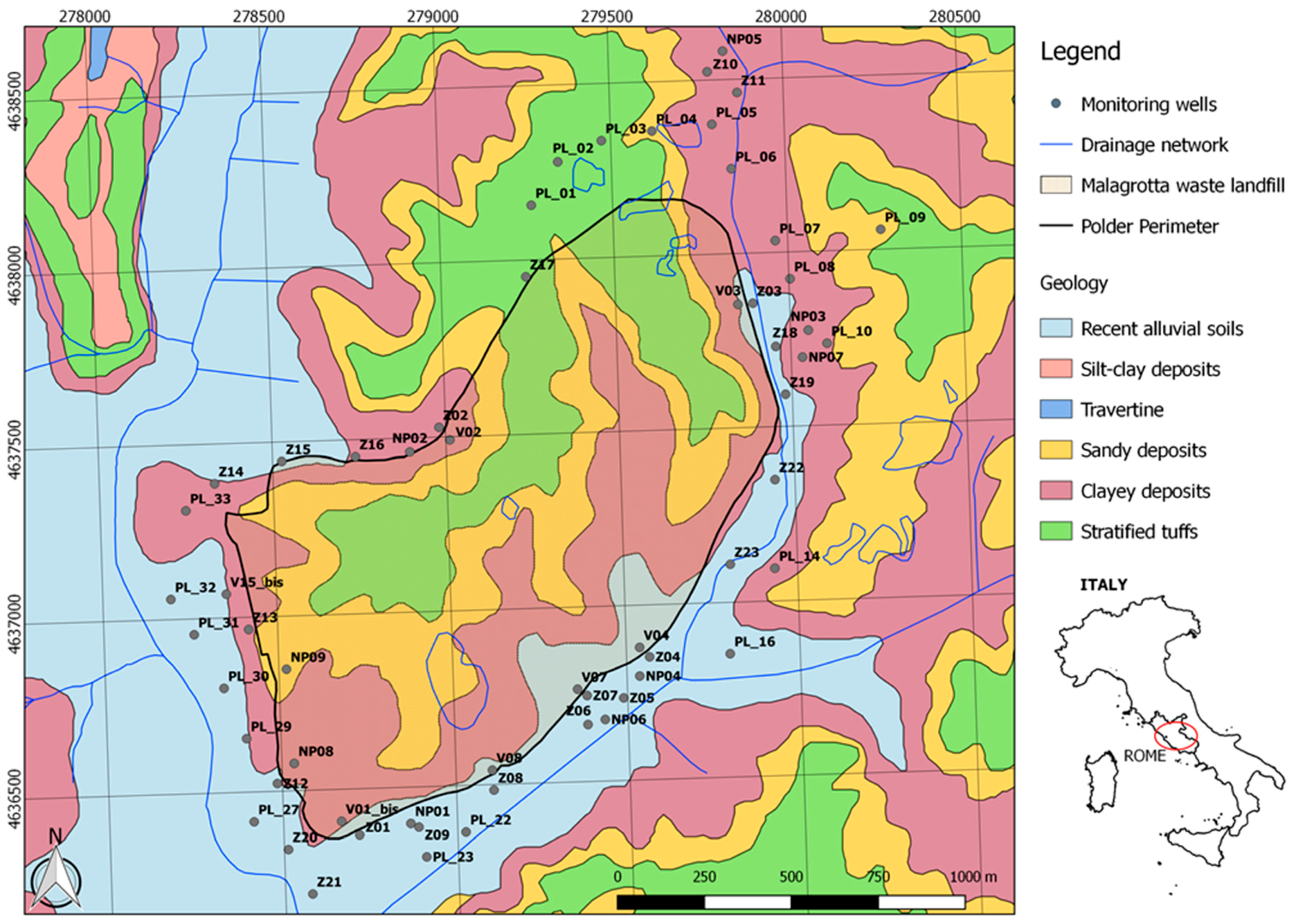
Rome’s municipal waste disposal site, Malagrotta, is located in the western part of Rome City, outside of the “Grande Raccordo Anulare” (GRA), a ring-shaped orbital motorway encircling the city. It is drained by the Galeria Streamlet tributary on the right bank of the Tiber River (Figure 1). It is a hilly area, a few hundred meters wide, with tops reaching a maximum height of 65–70 m a.s.l. (meters above sea level) and covering an area of about 160 ha.
The geology is mostly related to the presence of sediments belonging to the Ponte Galeria Formation (Middle Pleistocene Period). Local stratigraphy consists of an over-thickened basement of Plio–Pleistocene compact grey/blue silty clays. In the area of the landfill, overtly rusted clays and intercalated layers of sands, gravels, and silts are generally present [16,17].
Human activities have had a remarkable impact on this area, and they have produced remarkable changes on its original morphology. One example of the impact of human activities is the mining of gravel and sand related to construction works since 1950 [18,19].
More specifically, the stratigraphy from top to bottom is as follows:
- Gravelly soils: Marine and delta deposits, mainly coarse-grained (gravels and sands), with intercalating fine-grained materials layers and lenses (silts and clays);
- basement clays: Fine-grained marine deposits formed by clays with hydraulic conductivity in the order of 10−9 m/s.
On top of the reliefs, above the marine deposits, volcanic soils (muddy tuffs and tuffs) outcrop.
The contact surface between gravelly soils and the underlying clays basement is furrowed by depressions engraved by an ancient hydrographic network. The bottom of depressions created in the quarries is partially filled by heterogeneous non-thickened materials coming from the excavation sites and from the residues of the extraction activities.
The thickness of the alluvial soils is variable and can be in the order of tens of meters, as shown in the available stratigraphy of the study area. The permeability property of alluvial soils allows for the presence of a large aquifer, in which groundwater flows above the clay bottom boundary.
The static water level (SWL) measurements indicate that the water table ranges from 16 m a.s.l. and 25 m a.s.l. The main aquifer has a wide extension with general flow coming from northeast to southwest. The hydrogeological properties of the area are related to the stratigraphic overlap of gravels and sands on the grey/blue clay layers with very low permeability. Interbedded clayey levels sometimes sustain perched aquifers [20].
3. Materials and Methods
Low-flow purging procedure aims to collect groundwater samples which can be representative of the total mobile organic and inorganic loads transported through groundwater flow, with minimum physical and chemical alterations from sampling operations [4]. The aim of a low-flow purging process is to remove enough water from the well screen zone, in order to collect a sample that is representative of the aquifer conditions nearby the well.
According to this procedure, in the environmental monitoring network of Malagrotta landfill, the low-flow purging technique involved 59 monitoring wells, spread over the landfill area (Figure 1), along two groundwater sampling campaigns and was carried out in spring 2018 and summer 2018 (Table S1). Depth to water was measured before purging started and was then continuously recorded during the procedure using a heron water level meter instrument.
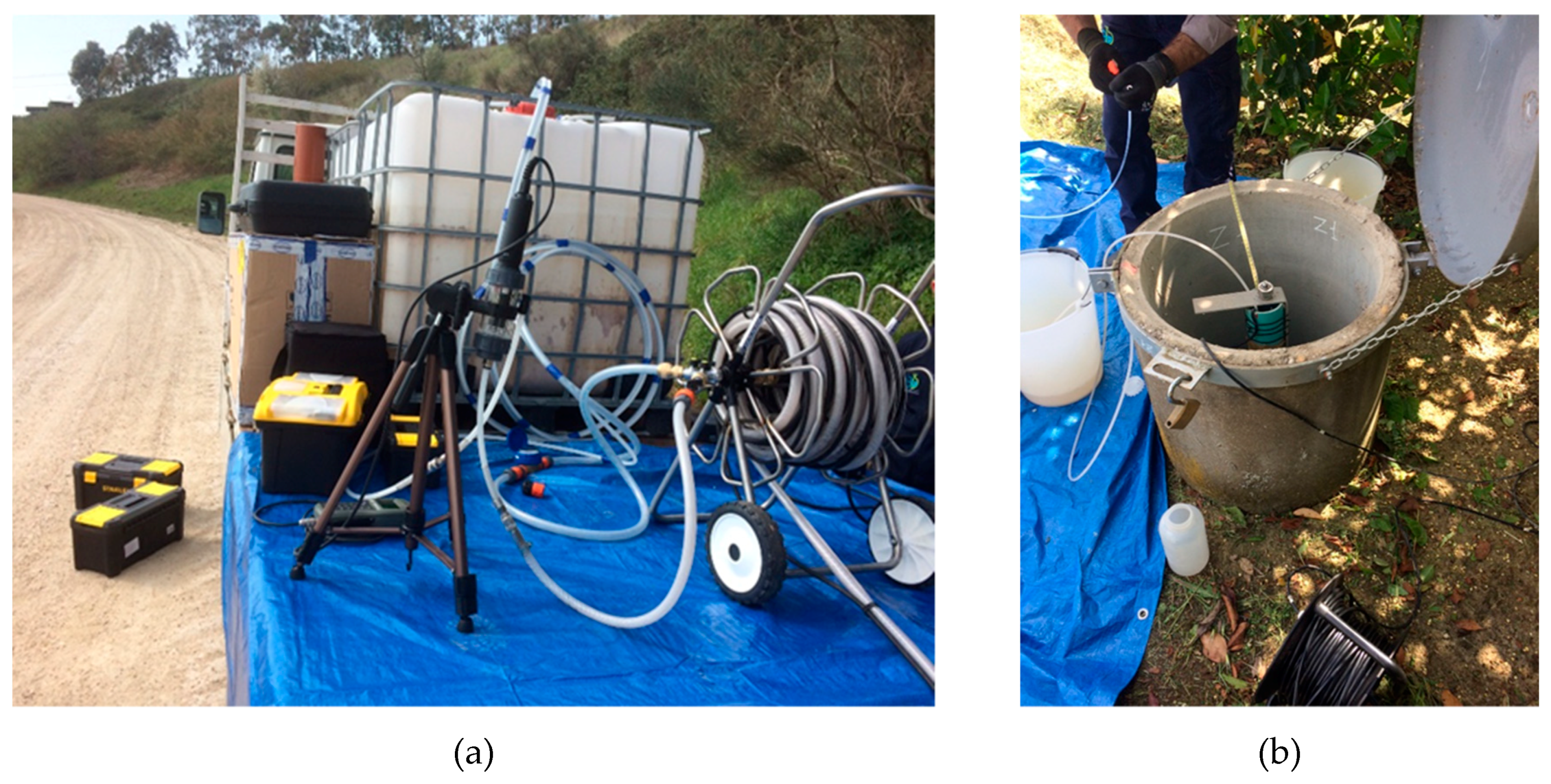
Monitoring well purging was carried out using a Grundfos Redi-Flo 2 submersible pump, with a flow rate ranging from 0.4 to 1 L/min. There was an exception for one well, where a rate of 1.4 L/min was set for operational needs. This low flow rate range was applied to minimize drawdown within the well with formation and mobilization of solids. The stabilization of groundwater chemical–physical parameters was done using a probe HI7629829/4-Hanna instrument. This allowed for the end of purging activities and the beginning of water sampling. A flow cell enclosed the probe during sample collection and field monitoring, preventing air from contacting the sample prior to the reading (Figure 2).
4. Theory
During low-flow purging, flow rates are low enough (<1 L/min) to minimize disturbance of well hydraulics (e.g., mixing, excessive screen intake velocity, screen dewatering, and turbidity) [2]. Moreover, all the monitoring wells taken into account in this study were fully penetrating and the water sample collection occurred after drawdown stabilization.
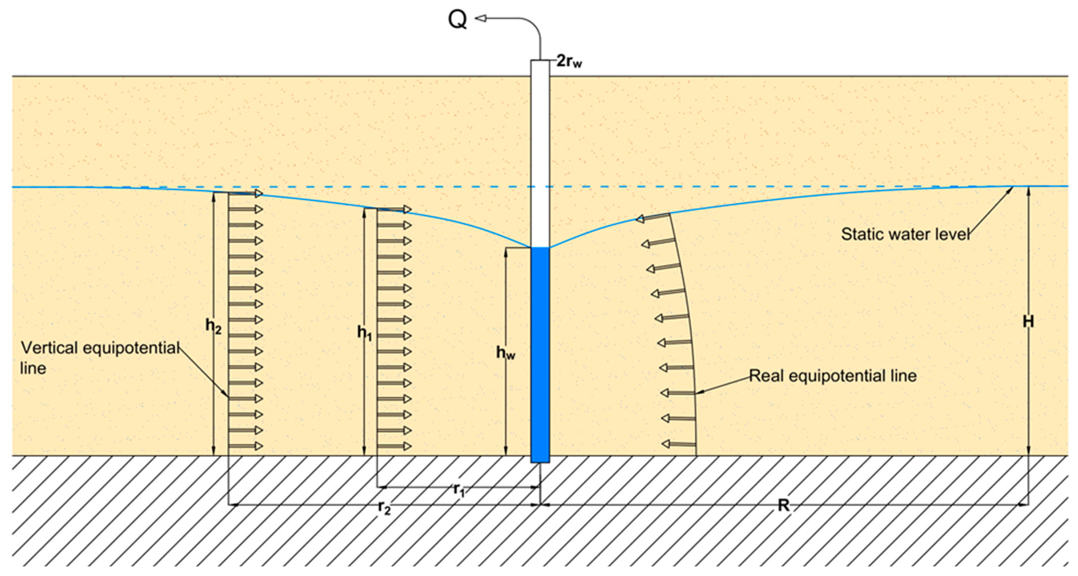
In such conditions, the vertical flow component is negligible compared to the horizontal one (vertical equipotential lines) and water is assumed to move horizontally through the well screen length (Figure 3). These conditions allow the application of the Dupuit’s hypothesis for steady-state radial flow in an unconfined aquifer [21] according to the formula:
where:
- Q = low-flow pumping rate (m3/s);
- K = aquifer hydraulic conductivity (m/s);
- R = influence radius (m);
- rw = radius of the monitoring well (m);
- H = undisturbed water column in the monitoring well (m);
- hw = steady-state water column in the monitoring well (m).
Solving Equation (1) for K gives:
Q and rw are previously known, whereas H and hw are measured respectively before and during the purging and sampling procedure. All monitoring wells penetrate the entire saturated thickness of the aquifer, according to Dupuit’s assumptions (1863).
The influence radius R, defined in Dupuit’s hypothesis as the distance from the well where drawdown is negligible, is considered steady after drawdown stabilization is achieved [22]. R depends on the aquifer hydraulic conductivity, and it increases as K increases. There are many empirical formulas that provide an estimation of the influence radius R. Among them, one of the most used is the Sichardt formula [23]:
Figure 4 is the graphical representation of Sichardt’s formula and shows the variability of R with drawdown (H − hw) for different values of hydraulic conductivity (K).
Sichardt’s formula applied with too much high drawdown values can lead to unreasonable results. R values lower than 30 m and higher than 5000 m should also be considered with caution. The value 3000 is a constant used when pumping is carried out in a single well. This constant ranges from 1500 to 3000 relating to the pumping system (single or multi-well) [23,24]. However, this parameter is irrelevant when estimating K, as results affect its variability (1500–3000 m) only by 1%–2%.
Nevertheless, considering the different case of low-flow purging and according to drawdowns observed during the monitoring campaigns, R values lower than 30 m have also been considered.
Considering that in an alluvial deposit the hydraulic conductivity K ranges from 10−7–10−6 m/s to 10−3–10−2 m/s and that drawdown values for low-flow purging are usually lower than the normal pumping rate for groundwater exploitation, an iterative procedure was set up in order to obtain the hydraulic conductivity value K.
In this research, for all the wells of the monitoring network rw is a constant and equal to 0.04 m.
Considering Equations (2) and (3), K is a function of R, which is a function of K again:
where H and hw are measured and Q and R have been fixed.
For this reason, the following iterative procedure has been imposed for the resolution of the Equation (4):
More specifically, Equation (5) is equal to:
According to previous studies [23,24], 30 m has been adopted as the first value (R = R0) in the iterative procedure (Figure 4).
In Equation (6), Sichardt’s formula has been properly modified considering a minimum threshold of R = 5 × rw in the case of very low drawdowns. In the procedure set, this change was necessary in order to obtain consistent values of R, which should take into account both well diameter and well losses.
Moreover, according to Yihdego’s experience (2017), the well radius rw may be large in comparison to R. In such cases, rw should be added to the Equation (3) for the determination of R [25].
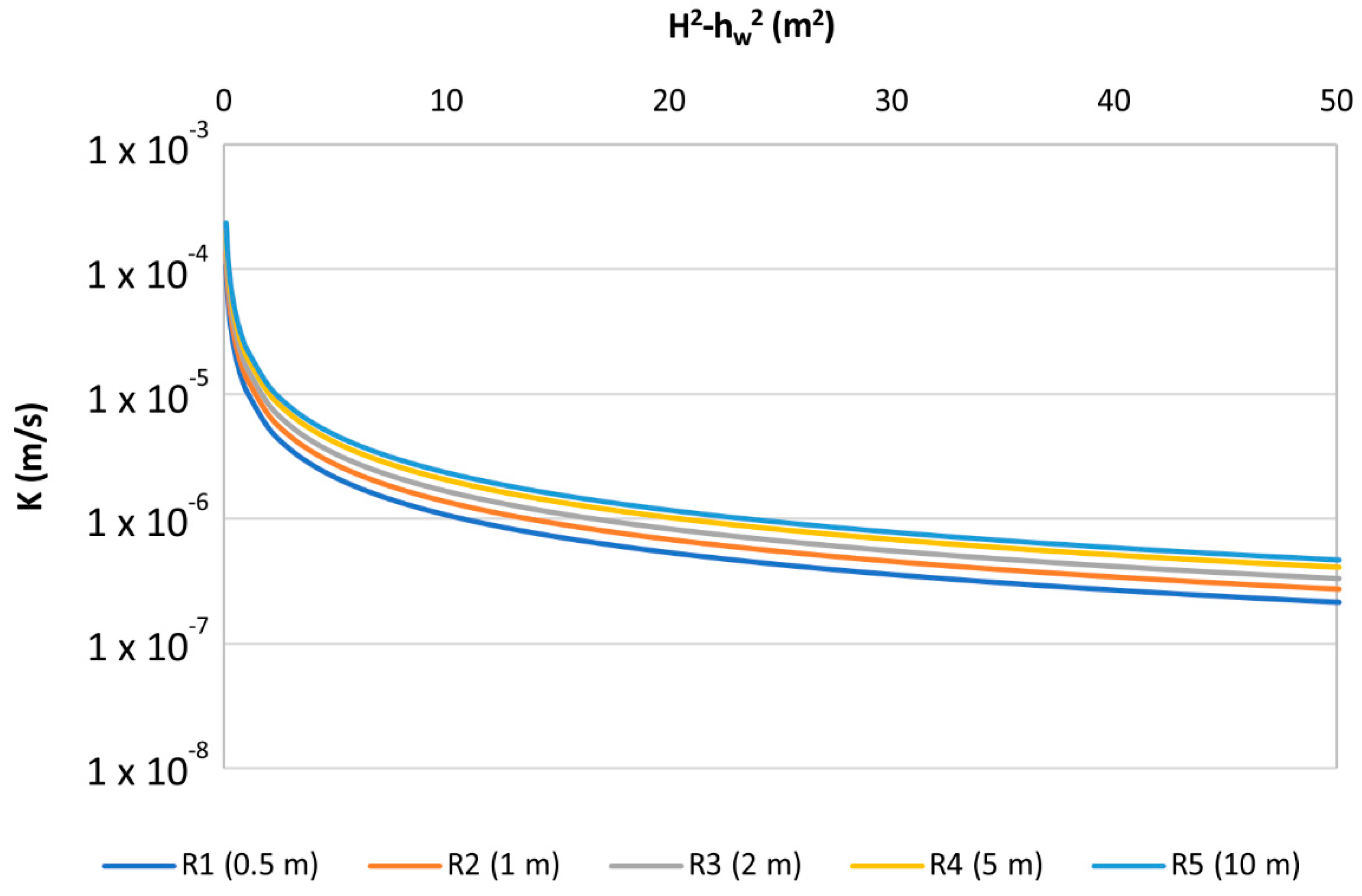
In addition, a sensitivity analysis of this parameter was carried out showing that the variability of hydraulic conductivity (K), due to the influence radius R, was very low if compared to the variation related to the term (H2 − hw2), as represented in Figure 5. The term H2 − hw2, which may be also written as (2H − Δh)Δh, is related both to the water column H, both to the drawdown Δh.
In this study, applying the abovementioned procedure, Ri and Ki values were obtained for data coming from the Malagrotta landfill area purging activities. The observed convergence of the iterative procedure was very rapid, requiring few iterations (up to 5 or 6) to reach an error ε < 0.01.
Results are presented further in the results section.
5. Results and Discussion
Low-flow purging data was used to calculate the hydraulic conductivity (K) using the water table measurements. All the monitoring wells penetrated the entire saturated thickness of the aquifer according to Dupuit assumptions [21]. In Figure 6 hydraulic conductivity values (m/s) come from the elaboration of low-flow purging data which was collected during two different campaigns, and refers to the 59 monitoring wells located in the study area. For further information about low-flow purging that was carried out, see the supplementary material (Table S1 and Table S2 show the following for each well: Depth of well, flowrates imposed, drawdowns measured, radius of influence and hydraulic conductivity obtained).
The hydraulic conductivity values coming from the first campaign dataset (spring 2018) were validated and were compared to those obtained in the second campaign (summer 2018) for each well. A single dataset, although useful, does not allow the identification of possible outliers due to errors that may occur during monitoring activities carried out in situ.
The term (H2 − hw2) in Equation (2) is related to the drawdown and to the thickness of the saturated layer (static water column H). When the measured drawdown is null the method cannot be applied because K would be infinite. This simply highlights that specific local hydraulic conductivity does not allow for the detection of appreciable drawdown in the application range of low-flow purging techniques. In these instances, a higher flow rate should be set. For this reason, in all cases where the drawdown was equal to zero, the hydraulic conductivity was estimated as higher than a threshold (>1.00 × 10⁻⁴ m/s).
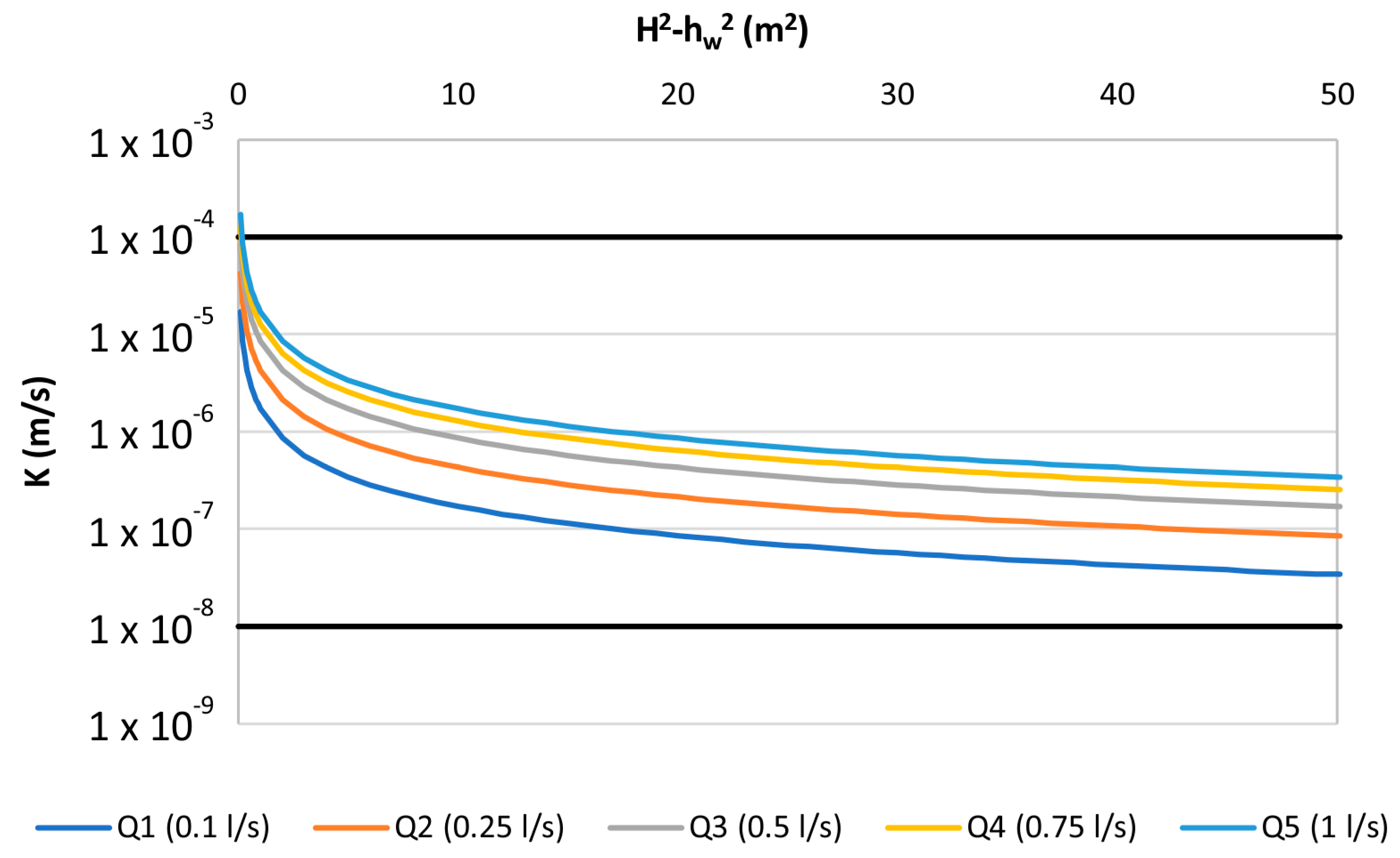
The threshold was chosen to be equal to the same order of magnitude related to the maximum value estimated for a drawdown (~1 cm) which is close to the operator accuracy. The comparison between the two estimated values obtained for the PL04 well shows the soundness of this choice (see Table S1). In fact, the estimated value in the first campaign (H = hw), was confirmed by the second campaign, in which lowering of the water table with the same flow rate (0.8 L/min) was recorded. In the same way, the method has a lower limit (1.00 × 10⁻⁸ m/s) for the hydraulic conductivity estimation as shown in Figure 7. As the flow rate varies in the range of low-flow conditions, the estimated hydraulic conductivity related to the variation of the term H2-hw2 remains within the range previously defined (1.00 × 10⁻⁸ m/s–1.00 × 10−4 m/s).
For estimated values within the range of 1.00 × 10⁻⁸ m/s–1.00 × 10−7 m/s, drawdowns observed are remarkable and higher than 2 m. This suggests that the lower limit of the methodology might be higher (1.00 × 10⁻⁷ m/s). Hopefully further site investigations will allow for a better definition of this aspect.
As shown in Figure 8, the monitoring wells of the Malagrotta landfill are distributed along the polder perimeter. Orange squared points represent wells where slug tests have been performed. Hydraulic conductivity values obtained with the proposed method generally matched between spring 2018 (first campaign) and summer 2018 (second campaign).
Hydraulic conductivity in the area ranged from a minimum of 2.5 × 10⁻⁸ m/s (Z04) to a maximum of 1.00 × 10⁻⁴ m/s. These values, shown in Table S1 and Figure 6, are strongly representative of the soil type characterizing the site under study. In fact, for alluvial deposits, various literature data confirmed K values ranging from 10−7 m/s to 10−2 m/s [26]. Results show the high soil heterogeneity of the study area which is typical of waste disposal sites because in Italy they are usually designed in previous quarry mining areas. Some areas present very different hydraulic conductivity values even if the monitoring wells are very close to each other.
The accuracy of the results is highlighted by the comparison between the values obtained from both purging campaigns for each monitoring well.
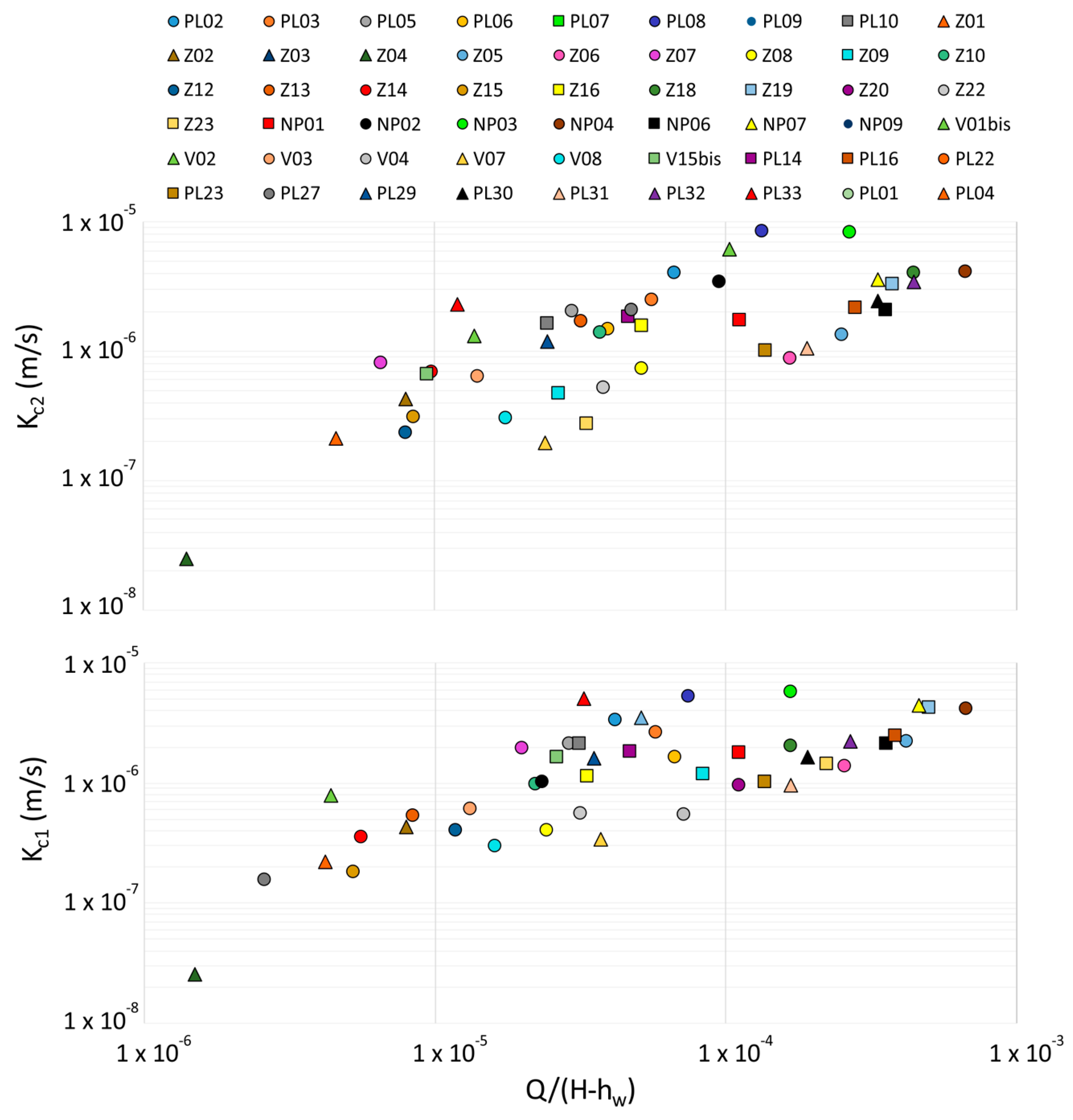
Values are strongly correlated, generally showing the same order of magnitude. In this regard, a scatter plot of estimated K values is shown in Figure 9. This figure shows wells with values obtained for both campaigns, i.e., for 52 monitoring wells, excluding those out of range (>1.0 × 10⁻⁴ m/s).
To assess the reliability of the proposed method, the Pearson index calculated for the two datasets is equal to 0.86, confirming a good correlation between the results obtained in the two purging campaigns (KC1 and KC2).
ρXY is a measure of the linear correlation between two variables X and Y, expressed as the covariance of the two variables divided by the product of their standard deviations (ρXY = σXY/σXσY).
Four classes related to different correlation degrees have been defined in order to quantify the number of wells in which K values have high correlation. Classes are as follows:
- Low correlation for |KC1 − KC2| > 1 order of magnitude (o.m.);
- Medium correlation for 0.5 < |KC1 − KC2| < 1 o.m;
- High correlation for 0.25 < |KC1 − KC2| < 0.5 o.m;
- Very high correlation for |KC1 − KC2| < 0.25 o.m.
About 65% of the wells showed a high correlation between the two datasets, whereas only about 2% showed a low correlation.
Comparison between the hydraulic conductivity estimated values and soil texture properties from stratigraphic reports referred to some of these wells and confirms the soundness of results from application of our proposed method. Starting from the available stratigraphy, two geological cross-sections were set up which are represented in the map (Figure 8). These cross sections (CS_01 and CS_02) are shown in Figure 10 and Figure 11 shows a comparison between the estimated K values for the two campaigns in the wells present in the geological sections. Each well crosses the entire saturated thickness of the aquifer. With regard to CS_01 in the NP08 well, it had the lowest hydraulic conductivity value (2.8 × 10⁻⁷ m/s) because of the presence of a significant thickness of Havana plio-pleistocene silty clay formation along the well screen. In the NP01 well, the presence of the alternation of silty sands and gravel—a more permeable soil—lead to different hydraulic conductivity values. For the NP09 well, with data related only to the second purging campaign, the highest hydraulic conductivity value was estimated (1.7 × 10⁻⁵ m/s). This result is in agreement with the soil type found (green sands with gravel and pebbles includes), which is more permeable than the others. Furthermore, from the comparison between stratigraphy info in CS_02 and the estimated hydraulic conductivity values obtained for wells NP08, V01bis, and NP01, similar considerations came out, confirming positive representativeness of the results. In fact, in V01bis, a value of intermediate hydraulic conductivity was estimated according to the type of soil found in this point (called alternation of sandy and clay silts).
The obtained K is a weighted average value of the different layers along the well screen as the horizontal hydraulic conductivity of the aquifer is expressed by the following equation:
Ht is the total thickness whereas hi is each layer’s thickness.
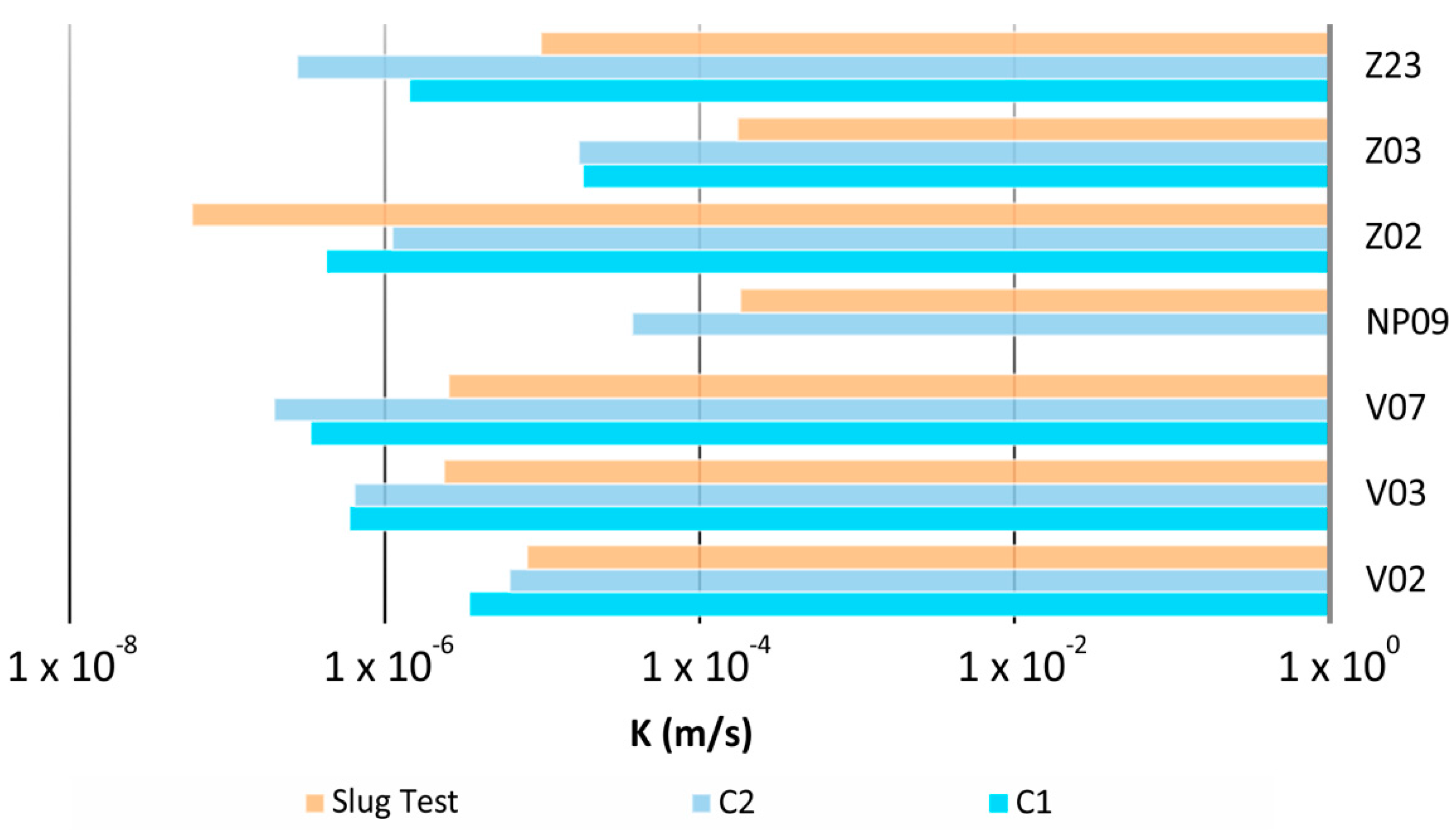
Slug test results referred to seven monitoring wells were compared with hydraulic conductivity values from the application of the proposed method (Figure 12). As previously described [27] slug tests consist of a single-well test carried out in a transitory regime, whose purpose is to determine the hydraulic conductivity of the aquifer in the immediate vicinity of the well. In fact, response to the abrupt variation of the water level introduced and the consequent value of hydraulic conductivity were strongly influenced by local hydraulic conditions.
Moreover, the slug test is meant to overestimate conductivity, particularly in an unconfined aquifer [15].
Tests were carried out on February 21–22, 2013 in wells V02, V03, V07 and NP09 inside the polder and in wells Z02, Z03, and Z23 outside the perimeter of the landfill using the Kansas Geological Survey (KGS) model for data analysis. The KGS model is a semi analytical solution for slug tests performed in confined and unconfined aquifers [28]. Examined results (Figure 12) show that in V03, V07, NP09, Z03, V02, and Z23 wells, K values estimated by the proposed method and slug test results were slightly lower, except in well Z02 where they differ more than one order of magnitude. Z02 is a well largely screened across the water table, whereas the KGS model was developed mainly for wells screened below the water table, accounting for elastic storability, anisotropy, partial penetration, and skin effects [29]. Skin effects of wells can influence the magnitude of hydraulic conductivity values calculated from slug tests, which refers to a disturbed zone around the well due to well drilling and installation or emplacement of a filter pack around the well [30]. Although the KGS model solution cited in this case study [27] takes into account several correctional factors such as skin effect, the general insensitivity of slug tests in wells screened across the water table to elastic storage mechanisms limits its use in this setting.
Thus, the recognition that a test is affected by a low K well skin effect can often only be based on a K estimate that is deemed too low for the interpreted stratigraphy [31]. Moreover, the KGS method is more rigorous and requires a large number of data on the construction parameters of the well which are often difficult to find [32]. This was the case for the Z wells in this study, as they are the oldest ones in the area.
On the contrary, if the steady-state, low-flow drawdown can be accurately measured, one can avoid complex analysis [9] related to slug test transient state. Low-flow purging data can provide a base for the estimation of hydraulic conductivity, especially for alluvial soil in contaminated sites.
6. Conclusions
This study aimed to propose an effective and reliable method for aquifer hydraulic conductivity (K) estimation using data coming from low-flow purging activities inside environmental monitoring procedures. The study area is located in the alluvial deposit of the ex-waste disposal site in Malagrotta (municipality of Rome), where there is a large monitoring network for environmental groundwater characterization (59 wells). Two low-flow purging campaigns were carried out in spring and summer 2018 to collect representative water samples. Collected data provided about 100 hydraulic conductivity estimations.
The method, based on the Dupuit’s Theory for steady-state radial flow in an unconfined aquifer, was applied to obtain hydraulic conductivity estimated values for all the monitoring wells, starting from the following assumptions:
- The chemical-physical parameters stabilization is coincident with the drawdown stabilization;
- During low-flow purging, flow rates are low enough (<1 L/min) to minimize disturbance of well hydraulics [2] and water is assumed to move horizontally through the well screen length.
Previous studies [23] suggest that values of the influence radius (R) lower than 30 m need to be considered with caution, but a sensitivity analysis carried out on this parameter showed its limited influence on final results. Moreover, considering the different case of low-flow purging and according to drawdowns observed during the monitoring campaigns, R values lower than 30 m were also considered.
An iterative procedure has been set up in order to obtain the hydraulic conductivity value K. The observed convergence of the iterative procedure was very rapid, requiring just a few iterations (up to five or six) to reach an error ε < 0.01. Hydraulic conductivity values, obtained for the study area, ranged from 3.95 × 10⁻⁸ m/s to 1.00 × 10⁻⁴ m/s. This latter value is a threshold, chosen when no drawdown has been measured during the purging procedures. In these cases, the specific high soil hydraulic conductivity did not allow for the application range of low-flow purging technique to detect a sensitive drawdown. For this reason, the proposed method turned out to be valid for a range of hydraulic conductivity from 1.00 × 10⁻⁸ m/s to 1.00 × 10⁻⁴ m/s. The range is very consistent with sandy texture of the alluvial deposits, highlighting the effectiveness of the method’s applicability for this type of hydrogeological settings.
Estimated K values in each well generally showed the same order of magnitude for both campaigns. In particular, the Pearson index calculated for the two monitoring campaigns was equal to 0.86, showing a high reliability of the estimations obtained. Hydraulic conductivity values, obtained with the proposed method, have been compared with slug test results obtained by the KGS model [28] and conducted in 2014 on seven monitoring wells. Results show that in V03, V07, NP09, Z03, V02, and Z23 wells, K values estimated by the proposed method and slug test results are similar even if slightly underestimated, except to Z02 well where they differ to almost two orders of magnitude. For this well, screened across the water table, the KGS model may have led to a misleading hydraulic conductivity estimation. On the contrary, as stated by Robbins et al. [9], if the steady-state, low-flow drawdown can be accurately measured one can avoid complex analysis related to slug test transient state. Moreover, the slug test is supposed to overestimate the conductivity, particularly in an unconfined aquifer [15].
These results show that low-flow purging data can provide a sound hydraulic conductivity estimation methodology for alluvial deposit, as groundwater monitoring activities with low-flow purging and sampling procedures are necessary in any potential site contamination case. The procedure proposed in this study can provide important groundwater flow information at a very low cost. In comparison with other kinds of hydraulic conductivity field estimation, this method allows one to obtain a better spatial representation of K parameter distribution, giving reliable knowledge of hydrogeological settings in very hydrogeological heterogeneous soils. In spite of their more detailed punctual characterization, other methods are usually more expensive but not as representative at the scale of potentially contaminated areas of interest. The best recommendation is to ensure that a steady state has been achieved in the well to control the chemical-physical stabilization and to measure flowrates and drawdowns. With these conditions respected, the proposed method can be very helpful by reducing operative timeframes, effort, and costs associated with additional site investigations such as slug tests.
Supplementary Materials
The following are available online at https://www.mdpi.com/2073-4441/12/3/898/s1, Table S1: Low-flow hydraulic conductivity values K estimated in Malagrotta landfill during monitoring campaign 1 (KC1) and monitoring campaign 2 (KC2), Table S2: Low-flow Radius of Influence values R estimated in Malagrotta landfill during monitoring campaign 1 (RC1) and monitoring campaign 2 (RC2).
Author Contributions
Conceptualization, G.S.; methodology, G.S., S.I., F.M.D.F.; validation, G.S., S.I. and F.M.D.F.; investigation, S.I. and F.M.D.F.; data curation S.I. and F.M.D.F.; writing—original draft preparation S.I. and F.M.D.F.; writing—review and editing, G.S. and F.F.; supervision, G.S. and F.F.; project administration, G.S. All authors have read and agreed to the published version of the manuscript.
Funding
This research received no external funding.
Acknowledgments
The authors thank Lab Ambiente & Sicurezza srl team for their support in collecting data.
Conflicts of Interest
The authors declare no conflict of interest.
References
- Mishra, P.K.; Kuhlman, K.L. Unconfined Aquifer Flow Theory: From Dupuit to Present. Adv. Hydrogeol. 2013, 9, 185–202. [Google Scholar] [CrossRef] [Green Version]
- Barcelona, M.J.; Varljen, M.D.; Puls, R.; Kaminski, D. Ground water purging and sampling methods: Hystory vs. Hysteria. Ground Water Monit. Remediat. 2005, 25, 52–62. [Google Scholar] [CrossRef]
- Dąbrowska, D.; Witkowski, A.; Sołtysiak, M. Representativeness of the groundwater monitoring results in the context of its methodology: Case study of a municipal landfill complex in Poland. Environ. Earth Sci. 2018, 77, 1–23. [Google Scholar] [CrossRef] [Green Version]
- EPA—Environmental Protection Agency. Low Stress (Low Flow) Purging and Sampling Procedure for the Collection of Groundwater Samples from Monitoring Wells; EPA: Washington, DC, USA, 2017.
- ISPRA—Italian Environmental Protection Agency. Manual for Environmental Surveys at Contaminated Sites. 2007; ISBN 88-448-0234-1. Available online: http://www.isprambiente.gov.it/it/pubblicazioni/manuali-e-linee-guida/manuale-per-le-indagini-ambientali-nei-siti (accessed on 4 March 2016).
- EPA—Environmental Protection Agency. Low-Flow (Minimal Drawdown) Ground-Water Sampling Procedures; EPA/540/S-95/504; US Environmental Protection Agency, Office of Research and Development, Office of Solid Waste and Emergency Response: Washington DC, USA, 1996.
- Shengqi, Q.; Hou, D. Optimization of groundwater sampling approach under various hydrogeological conditions using a numerical simulation model. J. Hydrol. 2017, 552, 505–515. [Google Scholar] [CrossRef]
- Tatti, F.; Papini, M.P.; Sappa, G.; Raboni, M.; Arjmand, F.; Viotti, P. Contaminant back-diffusion from low-permeability layers as affected by groundwater velocity: A laboratory investigation by box model and image analysis. Sci. Total Environ. 2018, 622–623, 164–171. [Google Scholar] [CrossRef] [PubMed]
- Robbins, G.A.; Aragon-Jose, A.T.; Romero, A. Determining hydraulic conductivity using pumping data from low-flow sampling. Groundwater 2009, 47, 271–286. [Google Scholar] [CrossRef] [PubMed]
- Harte, P.T. In-well time-of-travel approach to evaluate optimal purge duration during low-flow sampling of monitoring wells. Environ. Earth Sci. 2017, 76, 251. [Google Scholar] [CrossRef]
- McMillan, L.A.; Rivett, M.O.; Tellam, J.H.; Dumble, P.; Sharp, H. Influence of vertical flows in wells on groundwater sampling. J. Contam. Hydrol. 2014, 169, 50–61. [Google Scholar] [CrossRef] [Green Version]
- Britt, S.L. Testing the in-well Horizontal Laminar Flow Assumption with a Sand-Tank Model. Ground Water Monit. Remediat. 2005, 25, 73–81. [Google Scholar] [CrossRef]
- Sevee, J.E.; White, C.A.; Maher, D.J. An analysis of Low-Flow Ground Water Sampling Methodology. Groundw. Monit. Remediat. 2007, 20, 87–93. [Google Scholar] [CrossRef]
- Stone, W.J. Low-flow Ground Water Sampling—Is it a Cure-All? Groundw. Monit. Remediat. 1997, 17, 70–72. [Google Scholar] [CrossRef]
- Butler, J.J.; Healey, J.M. Relationship Between Pumping-test and Slug-Test parameters: Scale Effect or Artifact? Groundwater 1998, 36, 305–313. [Google Scholar] [CrossRef]
- Chiocchini, U.; Chiocchini, M.; Cipriani, N.; Torricini, F. Petrografia delle unità torbiditiche della Marnoso–Arenacea nella alta valle tiberina. Mem. Soc. Geol. Ital. 1986, 35, 57–73. [Google Scholar]
- Ventriglia, U. Idrogeologia Della Provincia di Roma; 1988–1990. Available online: http://www.provincia.rm.it/dipartimentoV/SitoGeologico/PagDefault.asp?idPag=20 (accessed on 20 January 2006).
- Barbieri, M.; Sappa, G.; Vitale, S.; Parisse, B.; Battistel, M. Soil control of trace metals concentrations in landfills: A case study of the largest landfill in Europe, Malagrotta, Rome. J. Geochem. Explor. 2014, 143, 146–154. [Google Scholar] [CrossRef]
- Nigro, A.; Barbieri, M.; Sappa, G. Hydrogeochemical characterization of Municipal Solid Waste landfill. Rend. Online Soc. Geol. Ital. 2015, 35, 304–306. [Google Scholar] [CrossRef]
- Galeotti, L.; Gavasci, R.; Prestininzi, A.; Romagnoli, C. L’impatto delle attività antropiche sulle acque sotterranee nell’area di Malagrotta (Roma). Geol. Appl. Idrogeol. 1990, 25, 219–232. [Google Scholar]
- Dupuit, J. Études Théoriques et Pratiques Sur le Mouvement des Eaux Dans les Canaux Découverts et á Travers les Terraines Perméables, 2nd ed.; Dunod: Paris, France, 1863; p. 304. [Google Scholar]
- Dragoni, W. Some considerations regarding the radius of influence of a pumping well. Hydrogéologie 1998, 3, 21–25. [Google Scholar]
- Cashman, P.M.; Preene, M. Groundwater Lowering in Construction, a Practical Guide; Spon Press: London, UK; New York, NY, USA, 2001. [Google Scholar] [CrossRef]
- Fileccia, A. Some simple procedures for the calculation of the influence radius and well head protection areas (theoretical approach and a field case for a water table aquifer in an alluvial plain). Acque Sotter. Ital. J. Groundw. 2015, 4, 7–23. [Google Scholar] [CrossRef]
- Yihdego, Y. Engineering and enviro-management value of radius of influence estimate from mining excavation. J. Appl. Water Eng. Res. 2017, 6, 329–337. [Google Scholar] [CrossRef]
- Freeze, R.A.; Cherry, J.A. Groundwater; Prentice-Hall Inc.: Englewood Cliffs, NJ, USA, 1979. [Google Scholar]
- Genon, G.; Zanetti, M.C.; Sethi, R. Relazione finale dei tecnici verificatori incaricati per la discarica di Malagrotta. Allegato 2—Determinazione Della Conducibilità Idraulica Mediante Slug Test, Technical Report, 2014; 107–113. [Google Scholar]
- Hyder, Z.; Butler, J.J.; McElwee, C.D.; Wenzhi, L. Slug tests in partially penetrating wells. Water Resour. Res. 1994, 30, 2945–2957. [Google Scholar] [CrossRef] [Green Version]
- Stanford, K.L.; McElwee, C.D. Analyzing Slug Tests in Wells Screened Across the Watertable: A Field Assessment. Nat. Resour. Res. 2000, 9, 111–124. [Google Scholar] [CrossRef]
- Henebry, B.J.; Robbins, G.A. Reducing the Influence of Skin Effect on Hydraulic Conductivity Determinations in Multilevel Samplers Installed with Direct Push Methods. Groundwater 2000, 38, 882–886. [Google Scholar] [CrossRef]
- Butler, J.J. Slug Tests in Wells Screened Across the Water Table: Some Additional Considerations. Groundwater 2014, 52, 311–316. [Google Scholar] [CrossRef] [PubMed]
- Fabbri, P.; Ortombina, M.; Piccinini, L. Estimation of Hydraulic Conductivity Using the Slug Test Method in a Shallow Aquifer in the Venetian Plain (NE, Italy). Acque Sotter. Ital. J. Groundw. 2012, 3, 125–133. [Google Scholar] [CrossRef]
Figure 1.
Geological framework of the study area and monitoring wells location.

Figure 2.
Field instrumentation used during sampling campaigns: (a) Flow cell and probe HI7629829/4-Hanna instruments; (b) Heron water level meter instrument.
Figure 2.
Field instrumentation used during sampling campaigns: (a) Flow cell and probe HI7629829/4-Hanna instruments; (b) Heron water level meter instrument.

Figure 3.
Steady-state radial flow in an unconfined aquifer induced by low-flow pumping in a well (modified from Dupuit, 1863). Q is the purging flowrate, H is the static water column (undisturbed), hw is the steady state water column in the well, rw is the well radius, R is the radius of influence, and hi is a water column at distance ri from the well during low-flow purging.

Figure 4.
Log–log graphical representation of Sichardt’s formula. Influence radius (R) variations with hydraulic conductivity (K) and drawdown (ΔH) (modified from Fileccia, 2005). Rmax and Rmin define the range in this specific application (low-flow purging).
Figure 4.
Log–log graphical representation of Sichardt’s formula. Influence radius (R) variations with hydraulic conductivity (K) and drawdown (ΔH) (modified from Fileccia, 2005). Rmax and Rmin define the range in this specific application (low-flow purging).

Figure 5.
(H2 − hw2) term vs. hydraulic conductivity (K) scatter plot with different influence radius R values (Dupuit’s Theory). H is the static water column (undisturbed) and hw is the steady state water column.
Figure 5.
(H2 − hw2) term vs. hydraulic conductivity (K) scatter plot with different influence radius R values (Dupuit’s Theory). H is the static water column (undisturbed) and hw is the steady state water column.

Figure 6.
Hydraulic conductivity (K) values estimated by low-flow purging in the Malagrotta landfill. KC1 and KC2 are the hydraulic conductivity values estimated for monitoring campaign 1 and 2, respectively. Q is the flow-rate imposed and H-hw the drawdown measured.
Figure 6.
Hydraulic conductivity (K) values estimated by low-flow purging in the Malagrotta landfill. KC1 and KC2 are the hydraulic conductivity values estimated for monitoring campaign 1 and 2, respectively. Q is the flow-rate imposed and H-hw the drawdown measured.

Figure 7.
(H2 − hw2) vs K scatter plot at different flow rate values Q. H is the static water column (undisturbed), hw is the steady state water column, and K is the hydraulic conductivity.
Figure 7.
(H2 − hw2) vs K scatter plot at different flow rate values Q. H is the static water column (undisturbed), hw is the steady state water column, and K is the hydraulic conductivity.

Figure 8.
Malagrotta landfill map showing the monitoring wells. CS_01 and CS_02 are two geological cross sections reconstructed.
Figure 8.
Malagrotta landfill map showing the monitoring wells. CS_01 and CS_02 are two geological cross sections reconstructed.

Figure 9.
Scatter plot of estimated hydraulic conductivity values from the two purge campaigns (a) and correlation degree statistics (b). KC1 and KC2 are the hydraulic conductivity values estimated for monitoring campaign 1 and 2, respectively. ρxy is the Pearson correlation index calculated for the two datasets.

Figure 10.
Geological cross-sections related to Figure 7 (cross sections 1 and 2).
Figure 10.
Geological cross-sections related to Figure 7 (cross sections 1 and 2).

Figure 11.
Comparison between the hydraulic conductivity values (K) in the two purge campaigns, for wells related to the geological cross sections 1 and 2 (a,b).
Figure 11.
Comparison between the hydraulic conductivity values (K) in the two purge campaigns, for wells related to the geological cross sections 1 and 2 (a,b).

Figure 12.
Comparison between the hydraulic conductivity values (K) obtained with low-flow purging during the two monitoring campaigns (C1 and C2) and values obtained with slug tests.
Figure 12.
Comparison between the hydraulic conductivity values (K) obtained with low-flow purging during the two monitoring campaigns (C1 and C2) and values obtained with slug tests.

© 2020 by the authors. Licensee MDPI, Basel, Switzerland. This article is an open access article distributed under the terms and conditions of the Creative Commons Attribution (CC BY) license (http://creativecommons.org/licenses/by/4.0/).
Share and Cite
MDPI and ACS Style
De Filippi, F.M.; Iacurto, S.; Ferranti, F.; Sappa, G. Hydraulic Conductivity Estimation Using Low-Flow Purging Data Elaboration in Contaminated Sites. Water 2020, 12, 898. https://doi.org/10.3390/w12030898
AMA Style
De Filippi FM, Iacurto S, Ferranti F, Sappa G. Hydraulic Conductivity Estimation Using Low-Flow Purging Data Elaboration in Contaminated Sites. Water. 2020; 12(3):898. https://doi.org/10.3390/w12030898
Chicago/Turabian StyleDe Filippi, Francesco Maria, Silvia Iacurto, Flavia Ferranti, and Giuseppe Sappa. 2020. "Hydraulic Conductivity Estimation Using Low-Flow Purging Data Elaboration in Contaminated Sites" Water 12, no. 3: 898. https://doi.org/10.3390/w12030898
Note that from the first issue of 2016, this journal uses article numbers instead of page numbers. See further details here.