Automatic Surface Water Mapping Using Polarimetric SAR Data for Long-Term Change Detection

1
Department of Earth and Space Science and Engineering, York University, 4700 Keele St., Toronto, ON M3J 1P3, Canada
2
Wildlife Research and Monitoring Section, Ontario Ministry of Natural Resources & Forestry, Trent University, 2140 East Bank Drive, Peterborough, ON K9L 0G2, Canada
*
Author to whom correspondence should be addressed.
Water 2020, 12(3), 872; https://doi.org/10.3390/w12030872
Submission received: 31 January 2020
/
Revised: 11 March 2020
/
Accepted: 13 March 2020
/
Published: 20 March 2020
(This article belongs to the Section Water Quality and Contamination)
Abstract
:Mapping the distribution and persistence of surface water in a timely fashion has broad value for tracking dynamic events like flooding, and for monitoring the effects of climate and human activities on natural resource values and biodiversity. Traditionally, surface water is mapped from optical imagery using semi-automatic approaches. However, this process is time-consuming and the accuracy of results can vary among image interpreters. In recent years, Synthetic Aperture Radar (SAR) images have been increasingly used. Microwave signals sensitive to water content make SAR systems useful for mapping surface water, saturated soils, and flooded vegetation. In this study, a fully automatic method based on robust stepwise thresholding was developed to map and track the change in the extent of surface water using Polarimetric SAR data. The application of this method in both Radarsat-2 and Sentinel-1 data in central Ontario, Canada demonstrates that the developed robust stepwise thresholding approach could facilitate rapid mapping of open water areas with a promising accuracy of over 95%. In addition, the time-series extent of surface water extracted from May 2008 to August 2016 reveals the dynamic nature of surface inundation, and the trend was consistent with the local precipitation data.
1. Introduction
Surface water bodies are the most significant resources on our planet. Human activities, climate, and other environmental changes have strong impacts on the locations and sizes of open water bodies, which in turn can affect surrounding environments, biodiversity, and human wellbeing [1,2,3,4]. Advanced remote sensing technologies provide an excellent opportunity to obtain spatially extensive and temporally repeated data relevant to mapping surface water [5,6,7,8]. With optical imagery, surface water is usually extracted based on the difference in the spectral reflectance between land and water. Water absorbs most of the radiation in near-infrared (NIR) and mid-infrared (MIR), whereas other cover types, such as vegetation, soil, and human infrastructure have a higher reflectance in these spectral ranges. In addition to the direct use of the surface reflectance in multispectral satellite imagery, several indices are commonly employed, including the normalized difference water index (NDWI) that uses the visible wavelength (0.52–0.60 micrometers) and NIR (0.77–0.90 micrometers) and modified normalized difference water index (MNDWI) that uses the visible and Mid-infrared wavelengths (1.55–1.75 micrometers) [9,10]. Despite the values of such metrics, the acquisition of passive optical data depends on weather conditions and solar illumination, which make it a challenge for them to be used in surface water monitoring. For example, flooding usually happens during the heavy rain, which makes it difficult for the optical sensors to obtain data of the earth surface covered by clouds [11].
As an active sensor, Synthetic Aperture Radar (SAR) can collect images day or night, and its microwaves can penetrate through most clouds, rain fields, water vapor, and aerosol layers. In particular, as water has a unique signature in SAR imagery, a calm water body behaves as a specular reflector with respect to the radar wavelength and thus appears as a low-intensity area in SAR images. This contrasts with the higher intensity of the rougher surrounding terrain, characterized by diffuse scattering [12,13,14,15]. However, the contrast is dependent on factors such as polarization and incidence angle of the emitted microwave radiation. For the current Radarsat-2 sensor with an incident angle ranging from 20 degrees to 54 degrees, calm water is considered to be specular reflection, and the backscatter is close to zero [16].
Several studies have been conducted to map surface water with SAR data through the thresholding techniques utilizing the low return signal behavior of open water. Specifically, methods include manually-defined histogram thresholding [17,18], the Otsu’s algorithm [19], radiometric threshold based on a gamma distribution [20,21], and threshold sets based on statistical analysis of the trainings [22,23]. Those approaches are not fully automatic, and some of them require additional processes to generate high accuracy surface water map, such as supervised classification approaches [22,24,25,26], region growing segmentation [20,23,27,28], and machine learning approaches [29,30,31]. Even with their success, these methods require time and human resources and thus are not operational [18,32]. In addition, some methods are incident angle-dependent, as higher incident angle data are selected for their high contrast between surface water and land [27,33]. Although higher accuracy has been achieved, it is not suitable for long term surface water mapping and emergency flood map production as the amount of the data is reduced. A fully automatic and incident angle independent process is thus much needed to support the timely production of surface water mapping.
In this study, a fully automated algorithm is developed to characterize effectively water bodies using Polarimetric C-band SAR data. Surface water extent was mapped through a robust stepwise automatic thresholding (SAT) approach and validated with a manual digitized surface water inventory. The SAT method was also compared with other commonly used approaches for surface water mapping using NDWI and Otsu’s method [34]. To further explore the potential of mapping surface water at a global scale, the algorithm was tested on both Radarsat-2 and Sentinel-1 SAR data. The algorithm was applied on a time series of Radarsat-2 data to map surface inundation dynamics.
2. Materials and Methods
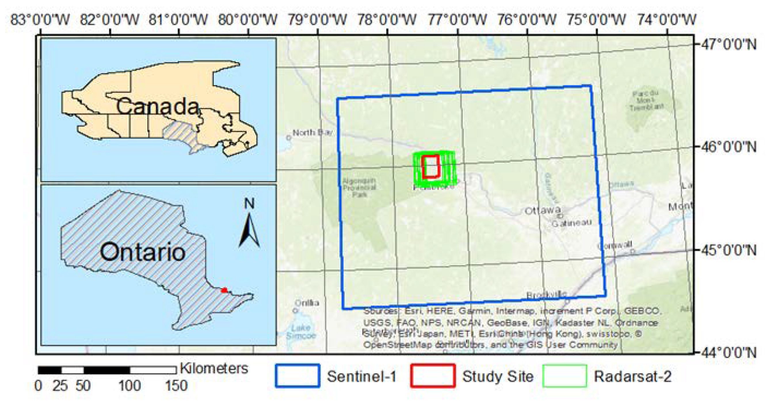
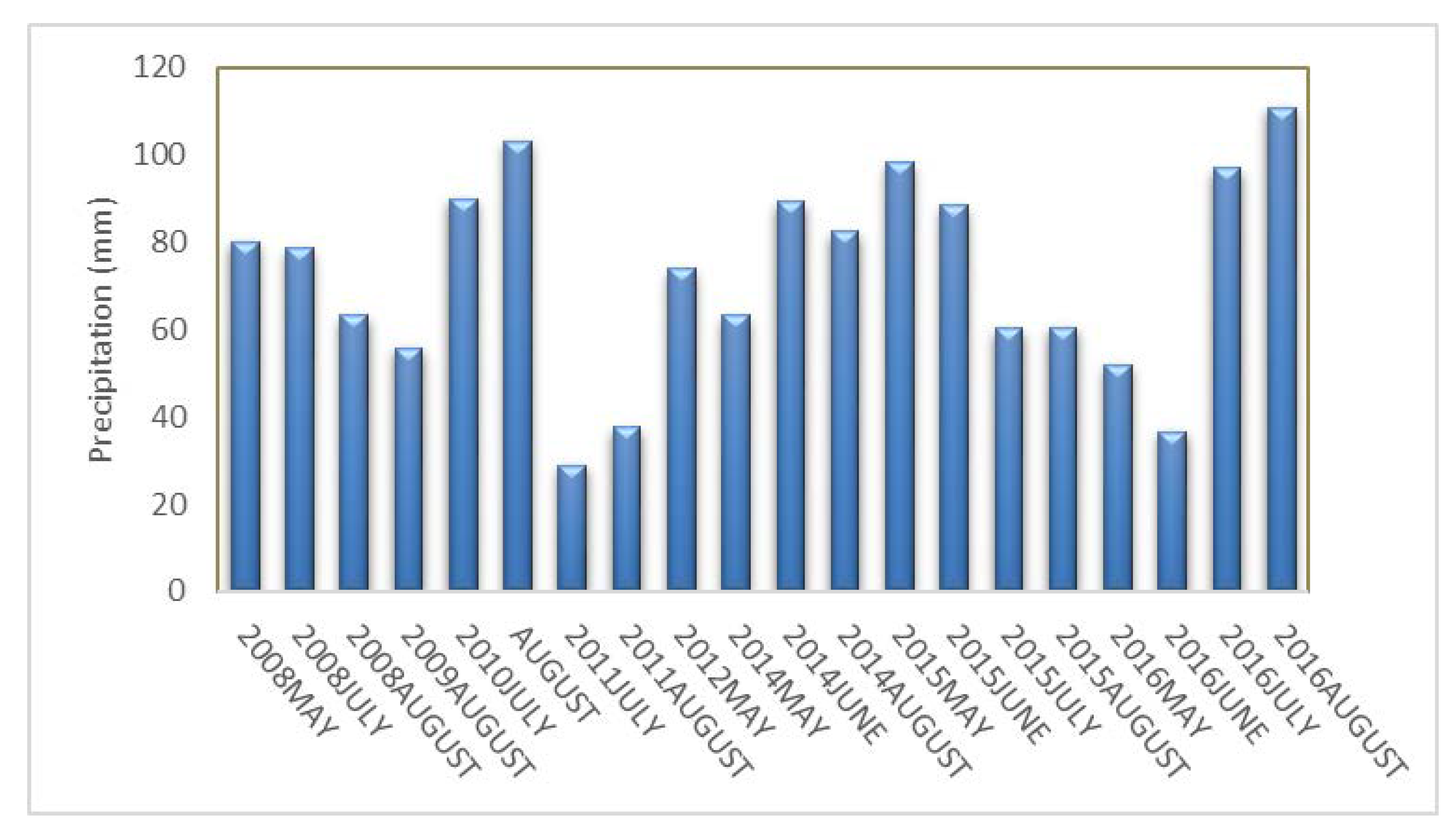
The study area is located in Ontario, Canada (77°28’21" W, 45°59’10" N)(Figure 1) within the Boreal Shield ecoregion, where the climate is generally continental with long cold winters and short warm summers [35]. The historical weather data show the monthly precipitation in the site ranges between 29 mm and 111 mm with the annual temperatures averaged at approximately 4.5 °C. Figure 2 shows the specific precipitation data in the area. Also, the area is within the western portion of black duck breeding range with the southern area covered by deciduous forest and transitioning to the northern boreal forest. The site was selected due to the availability of existing SAR and waterfowl data for individual wetlands, as needed to support initiatives of resources managers conducting wildlife-habitat assessments.
This study utilized a total of 51 scenes of C-band (5.405 GHz) Radarsat-2 Single look complex (SLC) images acquired from May 2008 to August 2016. The images all were acquired from Fine Quad (FQ) polarized mode, with a resolution of 5.2 m and 7.7 m in slant range and azimuth, respectively. Also, images were collected in both descending (acquisition time around 11:30 Coordinated Universal Time (UTC)) and ascending (acquisition time around 23:15 UTC) orbits, and from varies beam mode, including FQ4, FQ9, FQ14, FQ18, FQ23 and FQ28 to maximize the number of scenes for the temporal analysis. (Detailed information about the images is listed in Appendix A.)
Another C-band imager Sentinel-1A with a swath width of 250-km at fine spatial resolution was explored in this study. For algorithm testing, one scene of Dual-polarized (HH/VH) Sentinel-1 SAR data under interferometric wide-swath (IW) mode acquired on 9 June 2016, was first processed to Level-1 ground range detected (GRD), and then downloaded via python download from National Aeronautics and Space Administration Alaska Satellite Facility (NASA/ASF). The spatial resolution was 20.3 m and 22.6 m in slant range and azimuth, respectively, and the incident angle was between 32.9–43.1 degrees.
A digital elevation model (DEM) was employed to perform the terrain correction on the images, as the images were aligned and corrected for elevation interference to ensure that all SAR images were overlaid with each other and with the cartographic files. The DEM used for this purpose was the South Central Ontario Ortho-photography Project (SCOOP) grid (2 m), generated from the stereo imagery collected between April to May 2013.
To cross-validate the surface water mapped by SAR data, one scene of SPOT-7 imagery acquired on 03 May 2016 was also employed. The multispectral satellite imagery has four spectral bands, blue (450–520 nm), green (530–590 nm), red (625–695 nm), and near-infrared (760–890 nm), along with a spatial resolution of 6.6 m. The imagery has been ortho-rectified to be the same georeferenced as the SAR imagery.
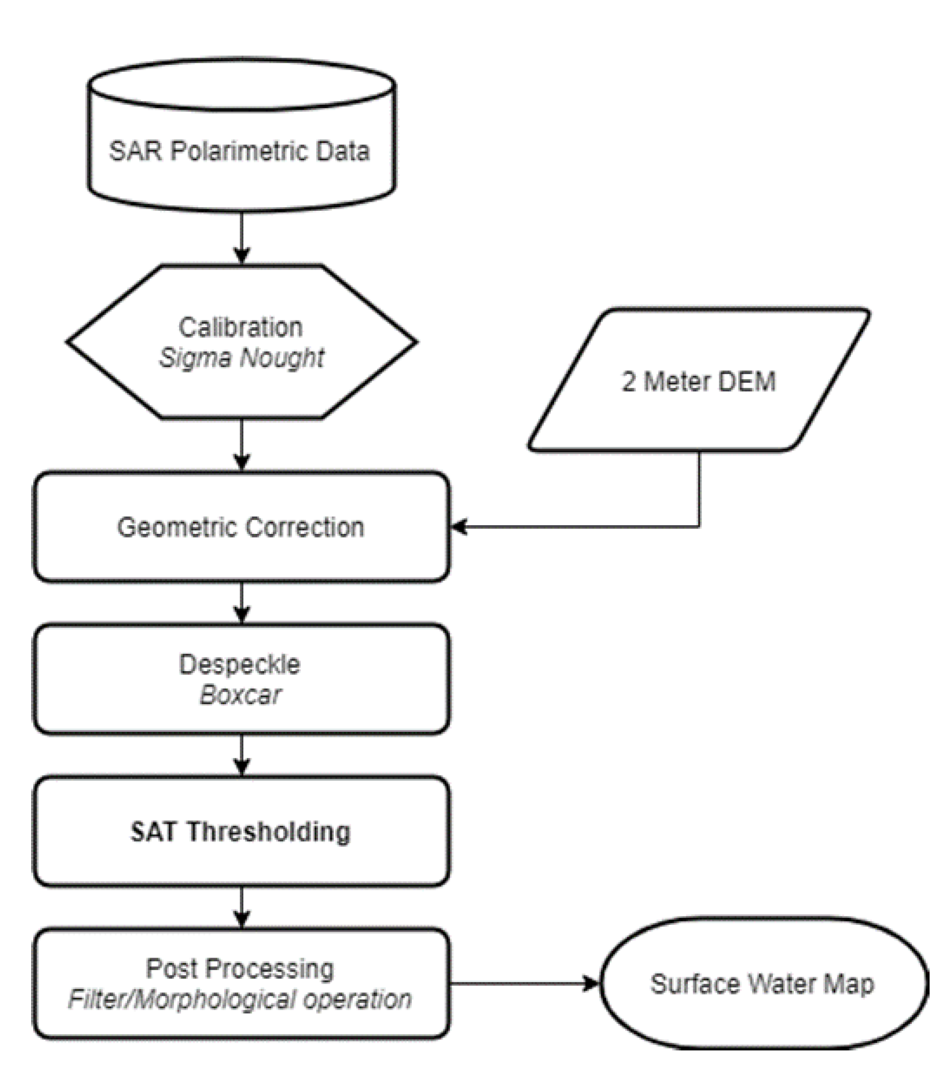
The proposed automatic algorithm consists of three steps: (1) pre-processing of SAR data to generate a backscattering coefficient, georeferenced with a provincial 2m LiDAR derived DEM to correct the relief displacement, and boxcar de-speckle filtering to remove the noise within the data, (2) SAT for generating the water extent map, and (3) post-processing of the image using morphological operations to remove an island within a lake and small misclassified areas (Figure 3). The HH polarization was used in this study as it provides the highest contrast between calming open water and land.
The pixel value of the SAR image was determined by the strength of the radar signal reflected from a unit area on the corresponding location in the scene, the backscatter coefficient β0 was used in calibration to convert the values from the digital number to the reflectivity of the surface objects. Parameter β0 was the radar cross-section per surface unit of the target with respect to the local incident angle. All SAR data were then converted from raw units to power units (decibels).
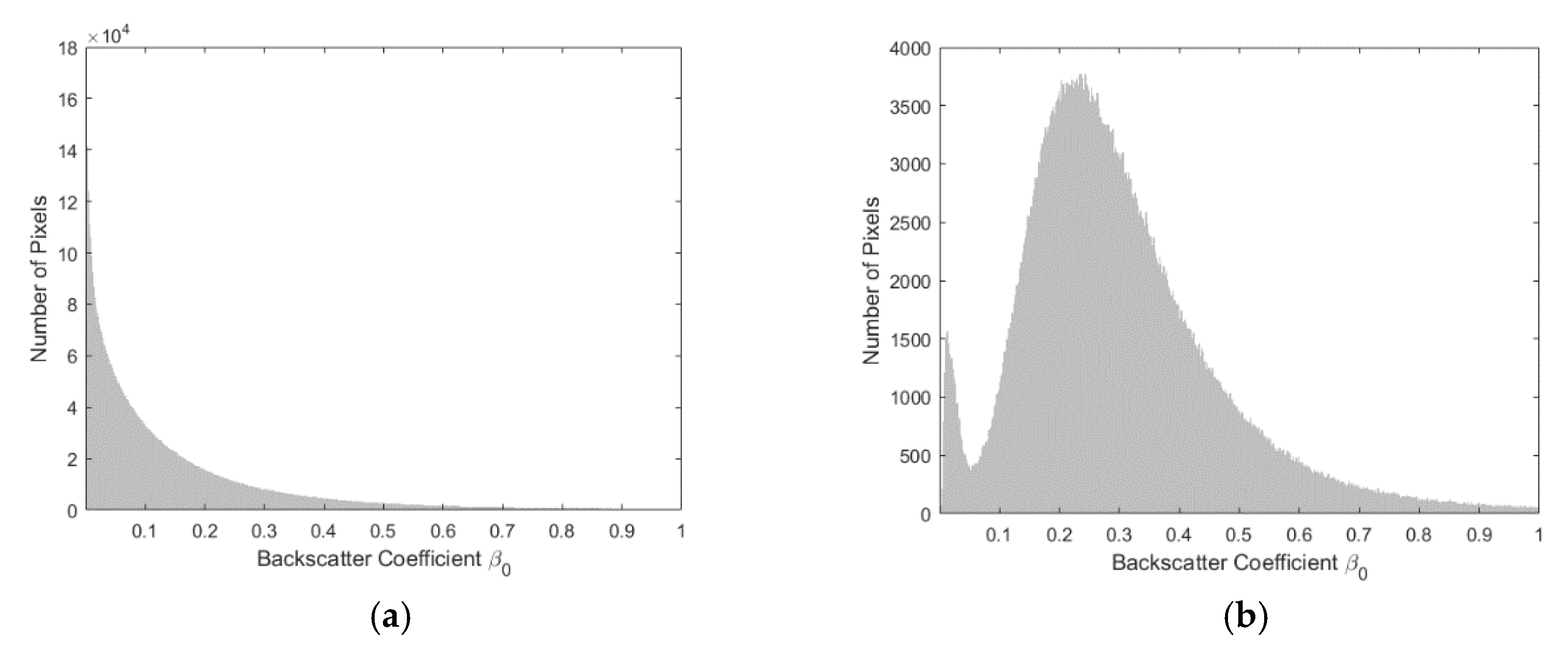
Due to the fact that the speckle effect caused by the coherent radiation used by radar systems was present, the de-speckle filter was employed to remove the salt and pepper noise while preserving edges and textural structures prior to data analysis. In this study, a boxcar filter with a 5-pixel by 5-pixel window was adopted, resulting in a unique valley-hill pattern in the histogram that represented a better distinction between water and non-water bodies, shown in Figure 4. The strategy of detecting the bottom of this valley has been proven to be a good threshold that separates water bodies (low backscattering coefficient) and non-water bodies [36]. Also, this pattern exists in all incidence angle of Radarsat-2 SAR data, not only the higher ones. Thus, the normalization between incident angles is omitted in this study. All the pre-processing procedures were designed as a workflow done automatically with python script utilizing the functions provided by PCI Geomatica.
To automatically determine the threshold value located at the valley (shown in Figure 4b), a step-wise method was developed. Specifically, a set of third-order polynomials was employed to fit the histogram in a manner of moving steps. The reason for this is that the third-order polynomial has the shape that best describes the histogram of backscattering coefficient after boxcar de-speckle, and easier to solve the turning points compared with the higher order polynomials. Also, as the image histogram was rough with notches throughout the curve, using local minimum detection would detect the bottom between any two adjacent notches, and yield multiple results that do not represent the true minimum, i.e., the threshold value. Moreover, due to the roughness of the histogram, using one polynomial to fit the entire histogram would yield a threshold value with significant uncertainty. Therefore, a step-wise polynomial fitting was the best choice to solve the threshold from the bottom of the valley.
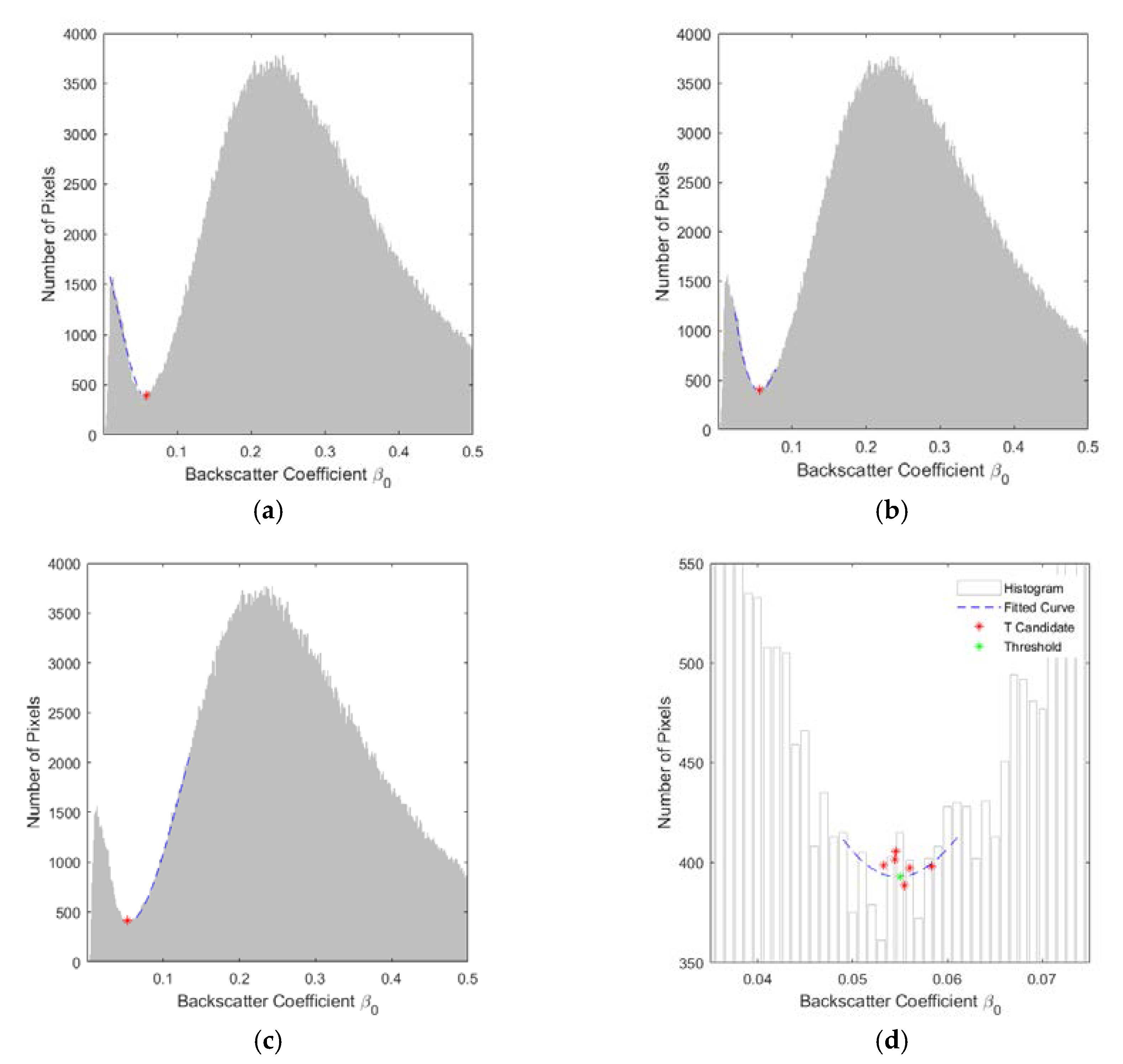
The iterative process started at the minimum value of the backscatter coefficient value. First, a partial histogram was extracted. Second, a third-order polynomial was fitted to the selected histogram. Last, the local minimum (turning point) was solved from the first derivative of the polynomial equal to zero. As the third-order polynomial was used, the smaller value of the solution was extracted and recorded as the threshold candidate (Figure 5a). Meanwhile, the difference between the two turning points are calculated, and 1/10 of the result value is stored as the step size. The process continued, and moved with the calculated step size to the next part of the histogram, another polynomial was fitted, and a second threshold candidate was solved (Figure 5b). The iterative process continued until the solved threshold value moved outside the fitting area of the selected histogram (Figure 5c). Finally, the optimal threshold value was obtained from fitting through the pre-determined candidates (Figure 5d). It is worth mentioning that when the slope of the two sides of the valley is different, i.e., very asymmetric shape, the candidates were scattered along with the histogram rather than clustered at the bottom of the valley. Therefore, fitting through all the candidates instead of simply calculating the average assures the optimal result.
After the threshold was determined, each pixel in the SAR image was classified into either water or land, depending on whether its value was smaller or greater than the threshold, respectively. Post-processing was used to refine the classification result. First, morphologic dilation [37] was performed by filling any holes or gaps that appeared as “islands” inside the big water bodies. A size filter was applied to remove any isolated water regions that were smaller than 3 pixels.
To further test the proposed automatic thresholding method on different sensor types, one scene of Sentinel-1 data from the same area was employed. For sentinel-1 data pre-processing, the Science Toolbox Exploitation Platform (SNAP) Toolkit developed by the European Space Agency was used. The workflow was built to generate the HH intensity image from high-resolution Level-1 ground range detected products, and then the image was pre-processed for geocoding, terrain-flatten, and the signal was corrected to sigma naught backscatter coefficients (β0). The boxcar de-speckle filter with 5 × 5 kernels was used to reduce speckle noise. Terrain flattening and terrain correction was conducted using the recently released Shuttle Radar Topography Mission (STRM) 1 arc-second (approximately 30 m) digital elevation model (DEM) (SRTMGL1).
In addition, the Otsu thresholding method [38], one of the most commonly used automatic image thresholding techniques, was utilized to obtain another surface water map and compared with the one generated with the proposed SAT method. The threshold value was determined through an iterative process that minimizes the within-class variance at the same time it maximizes between-class variances.
To access the binary classification generated by the SAT, both qualitative and quantitative analyses were conducted based on the manually digitized shapefile and 7-m SPOT true color imagery. As the shape and the presence of the wetland can be different between the creation dates, the reference data were visually interpreted using the SPOT imagery.
The last step was to process a total of 51 Radarsat-2 scenes of the overlapping area with the above-mentioned procedure. As the study area has a flat terrain, the displacement introduced by different incident angles was less than one pixel (~7-m) after geo-referencing with the 2-m DEM. Surface water bodies were extracted with the proposed SAT method, and the total area of the delineated surface water extent was calculated and plotted against the precipitation data to conduct the time series analysis.
3. Results
3.1. Surface Water Classification
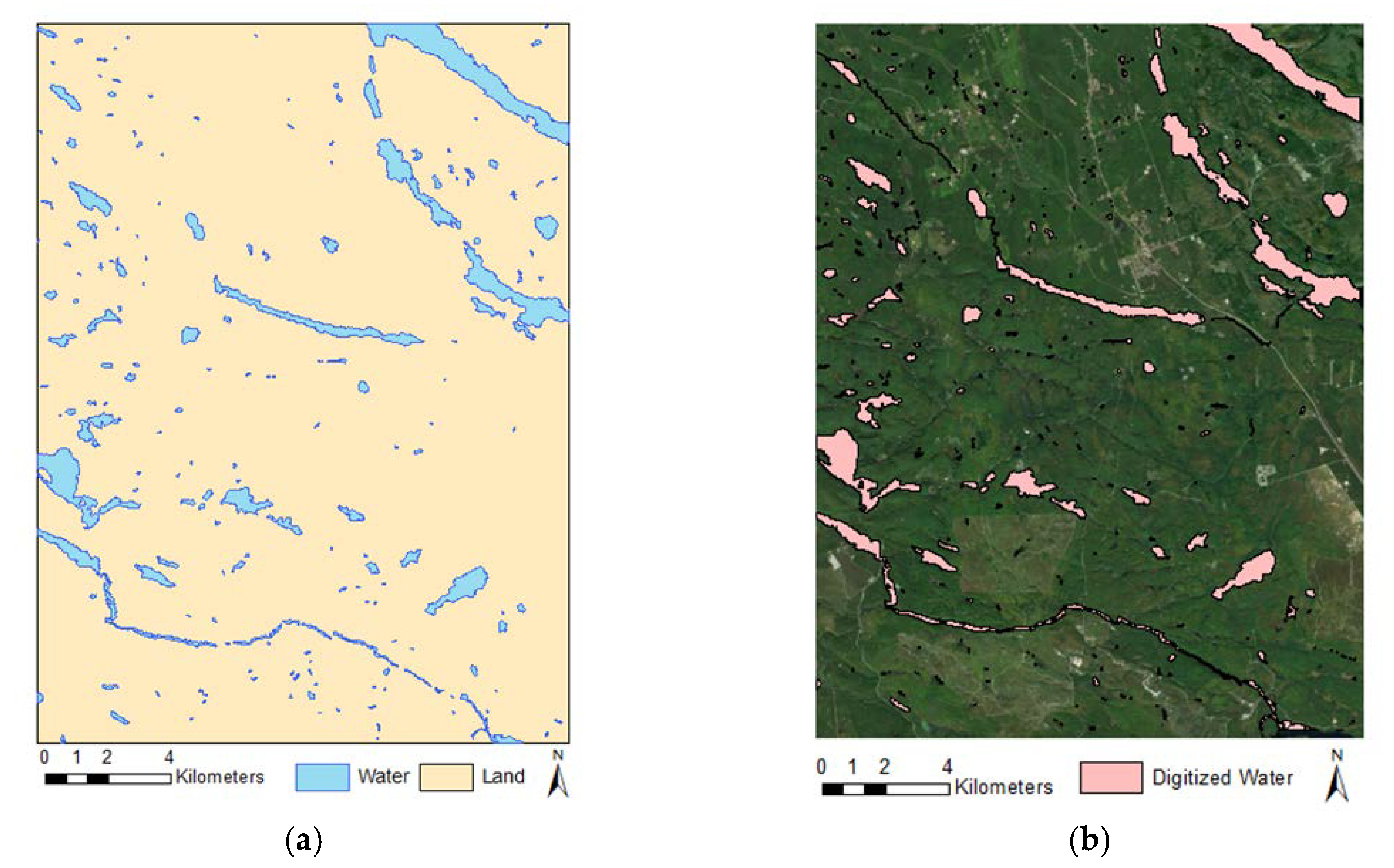
The surface water map generated from proposed SAT method with Radarsat-2 data, acquired on 5 August 2016, is shown in Figure 6a. For comparison, the corresponding manual digitized polygons are shown in Figure 6b. The majority of surface water bodies were successfully identified and extracted, with the kappa coefficient k = 0.9822. A few linear water streams are missing in the classification results as omission errors, and a few commission errors are evident near the bottom of the site, which appears to be inundated water or flooded vegetation falsely identified as open surface water.
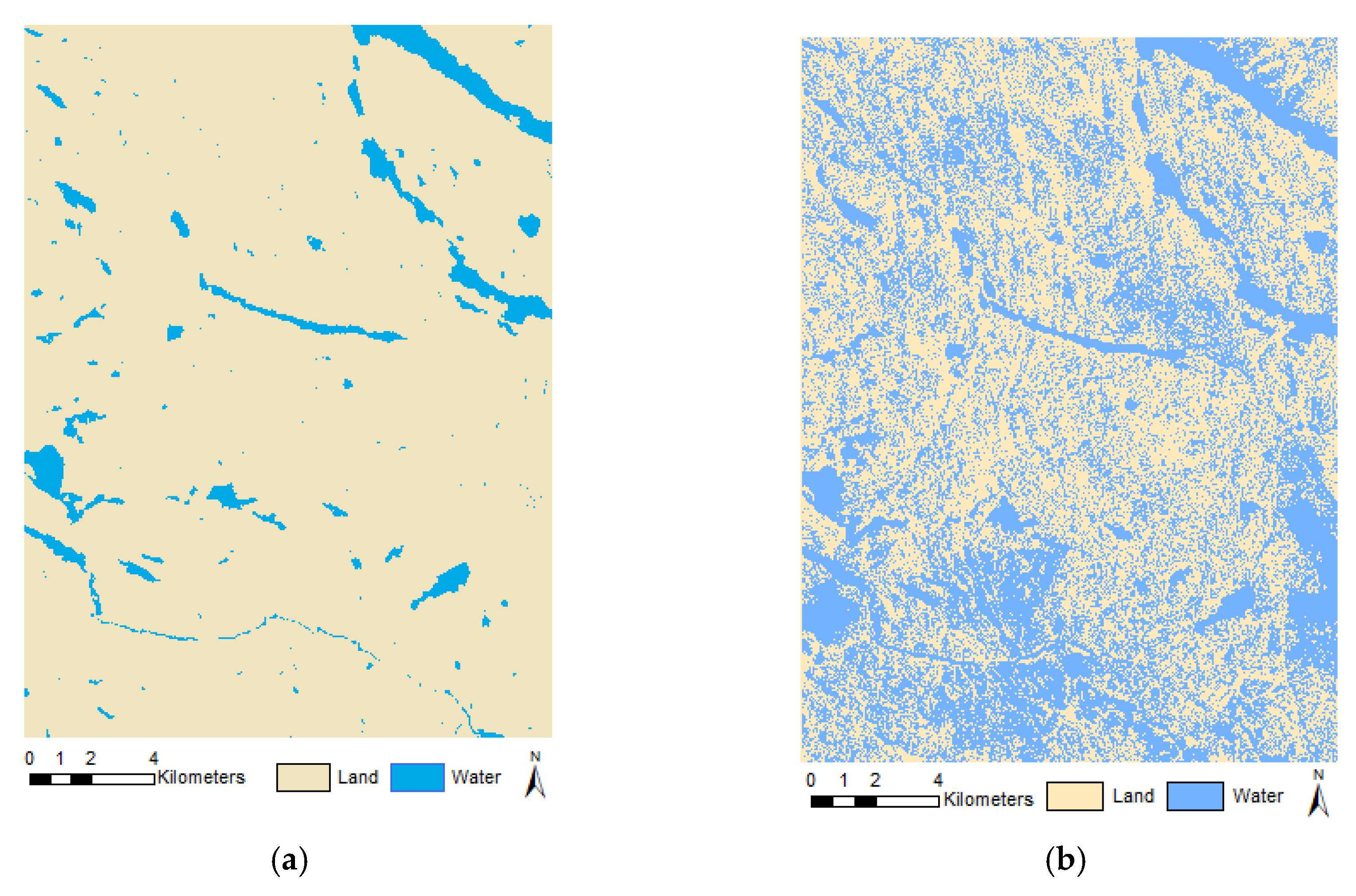
The surface water map generated from Sentinel-1 data with proposed SAT (Figure 7a) is consistent with the manually digitized polygons over large water bodies. Similar to the Radarsat-2 result (Figure 6a), the majority of surface water bodies were successfully identified and extracted with k = 0.9797, while part of the water streams was missing in the classification results as omission errors. On the other hand, the water/land class derived from the same Sentinel-1 data with Otsu thresholding is illustrated in Figure 7b, and the surface water extent was not successfully extracted, with k = −0.7181. Although all water bodies are identified, the majority of the land is falsely classified as water.
3.2. Accuracy Assessment
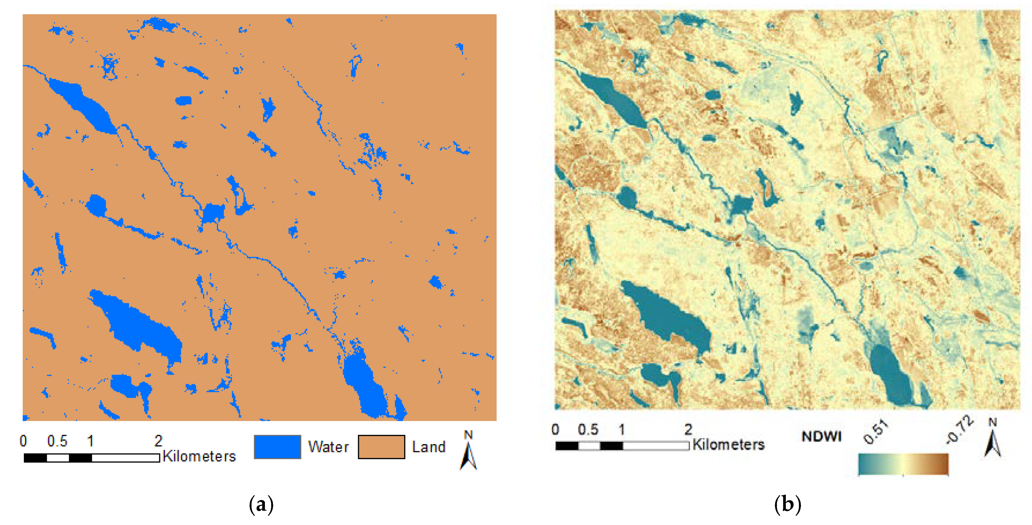
One scene of a high-resolution SPOT multispectral image was chosen to be within the closest date with the Radarsat-2 data for comparison and accuracy assessment. Figure 8a shows the water bodies derived from SPOT NDWI image using Otsu thresholding and illustrates that large size open water bodies, such as the lakes, have been successfully delineated with k = 0.9586. Also, the linear streams which connect the lakes have been differentiated from the land. However, the built-up land features (top left) are falsely identified as surface water objects. The built-up land features have the same positive values as water features in the NDWI image. This is due to the fact that the index is able to efficiently suppress vegetation and soil to negative values, but fails to separate the built-up land background from the positive value range.
To quantitatively evaluate the classification result, a manually digitized shapefile was used to validate the accuracy of classifications and the results are shown in Table 1. As illustrated in Table 1, the overall accuracy for both Radarsat-2 and Sentinel-1 SAR data exceeds over 95%, and SAR water class has higher total accuracy than the one generated from the NDWI image. The water classification of Sentinel-1 data using Otsu’s method has a total accuracy of 60.34%.
For the accuracy of SAR derived water class, the false identification rate is higher than that derived from NDWI image, indicating more land features may have been falsely identified as water (i.e., commission errors were high).
3.3. Time-Series Analysis
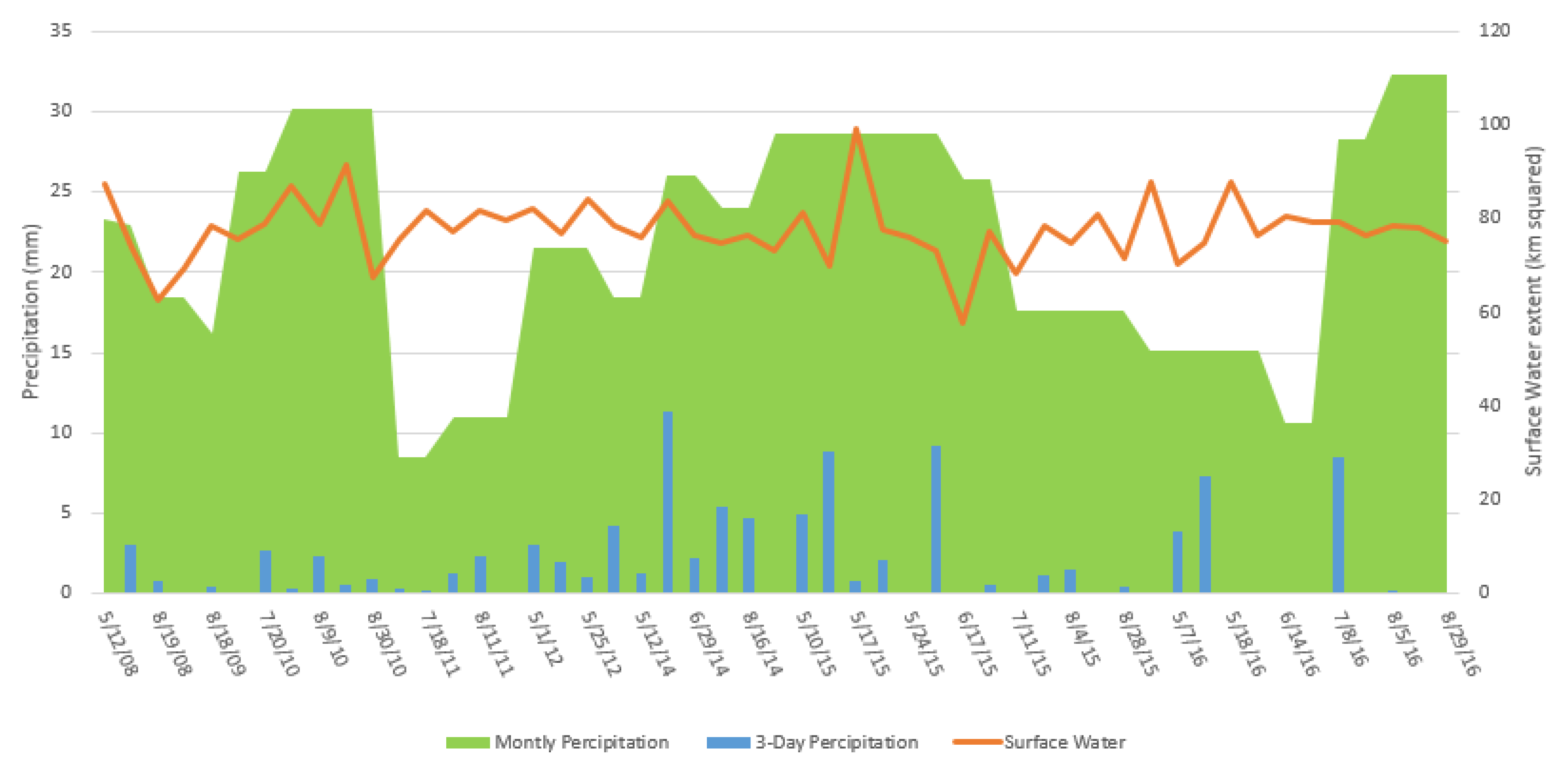
The time-series extent of surface water was extracted using the Radarsat-2 data from May 2008 to August 2016 shows the dynamics of surface water. As shown in Figure 9, the surface water extent generally varies in relation to monthly accumulated precipitation as measured at the local weather station. Decreases in precipitation were associated with a lower area of surface water for several of the observed months (August 2008, May 2014, August 2014, and June 2015). The area of water bodies follows the rate of 3-Day accumulated precipitation reasonably well. In general, the area of water bodies increases after an increase of 3-Day accumulated precipitation and the change in surface water agrees with the change in precipitation. The area of water bodies follows the rate of 3-Day accumulated precipitation reasonably well. In general, the area of water bodies increases after an increase of 3-Day accumulated precipitation and the change in surface water agrees with the change in precipitation.
4. Discussion
For the entire Radarsat-2 dataset (51 scenes), with the average imagery size of 2700 pixels by 3800 pixels, the proposed method computes the series of water maps in 559.26 s on a computer equipped with Intel® i7-6700 3.4 GHz and 16 GB RAM. Among the whole processing time, SAT thresholding takes 248.92 s, post-processing takes 12.95 s, and writing the image file takes 297.39 s.
The proposed SAT thresholding method successfully extracted the majority of surface water bodies. This can also be observed from the histogram (Figure 10), as the proposed method detects the threshold close to the bottom of the valley (indicated by the blue line), while the Otsu’s method locates the threshold near the peak (indicated by the red line). It can be observed that the surface water bodies with the flooded areas only cover a minor portion in the study area, producing a different histogram from the water dominated studies as shown in Martinis et al., 2009 [27], and the Otsu method failed to properly classify the surface water from the SAR data within our study area.
It is worth mentioning that Otsu thresholding is more effective to separate water and non-water classes when the histogram exhibited as a bi-modal histogram, i.e., two distinct objects presented as one maximum for water and one maximum for land. This can be observed in the NDWI image, and Otsu method is able to separate the two classes with an accuracy of 96%. On the other hand, the histogram of boxcar filtered SAR data only has a single modal presented, as shown in Figure 10, using Otsu yield low classification accuracy, around 40%. To better align with the literature, the de-speckle filter employed in Otsu thresholding for SAR data is Lee filter, instead of the boxcar filter used by the proposed method, and the classification accuracy raised to a reasonable 60%.
A variety of factors might complicate the derivation of water surfaces from SAR data. The low backscattering from some bare agriculture fields and radar shadows led to the overestimation of the water extent. As well, some inundated water resulting from heavy precipitation appeared in the SAR data, but was not evident as water in the reference data. For the water surface derived from the NDWI image, the higher commission errors than the omission errors are possibly due to flooded vegetation being classified as water. For the water surface derived from the SAR data, omission errors were observed from smooth objects like pavement and bare soil. Future studies can include additional road masks to reduce the overestimation introduced by roads in urban areas. Omission errors were observed from flooded vegetation close to rivers and lakes (left side of Figure 5b). This finding is consistent with previous studies that have found fully Polarimetric data were preferred for detecting flooded vegetation [25,39]. Furthermore, the Radarsat-2 detected inundated water areas unidentified in the provincial inventory are typically smaller water bodies. Those areas can be a potential breeding area for water birds.
Notably, part of the commission errors may also result from the difference in acquisition time between the spectral image and the SAR image. The reference manual digitized shapefile was generated from interpretation from the recent spectral image, and the actual boundary observed from SAR data did not precisely follow the same edges from the spectral image. Also, the influence of roughening of the water due to wind on the radar backscatter results in diminished water/land contrast, which can affect the classification accuracy. Future study will cooperate with multi-temporal filters [40] and non-local speckle filters [41] to potentially reduce the speckle-noise while the time-sensitive edges are adapted.
5. Conclusions
An automatic surface water extraction algorithm was developed in this study. The result of developed fully automatic SAT method demonstrates the ability to map the dynamics of surface water with promising accuracy. The preprocessing of SAR data and classification is fully automatic utilizing the Geomaticas and the SNAP toolbox and Python packages. The whole process is fully automatic, and the default values that have been encoded are found to be efficient in extracting surface water extent for different scenes. Our findings demonstrate that using an SAT technique can automatically generate the highly accurate surface water extent from C-band SAR data (Radarsat-2 and Sentinel-1) in an efficient and timely manner. Based on the accuracy assessment, 98% of the water bodies have been successfully extracted, and the surface water extent closely follows the boundaries of the main water bodies, such as the lakes and rivers. Omission errors observed from small, linear targets, i.e., streams and river, and commission errors are identified from roads and inundated vegetation. Future study can include local road masks to reduce the overestimation, and test the effects of non-local speckle filter for minimizing the influence of roughening of the water due to wind. Also, it worth mentioning that the proposed method has only been applied to flat terrain, and additional assessments should consider outcomes for rough terrain. Another valuable finding of this study is that time-series results reveal seasonal dynamics of inundation, and show a strong relationship of the response in surface water extent to the changes in precipitation.
Using SAR data thus permits a detailed timely fashioned surface water map for wetland habitat monitoring that was previously missed from inventory data and land classification map. The fully automatic algorithm developed in this study can be implemented in an operational system to generate provincial or national scale, and benefit the long-term water monitoring frameworks for wetland and management. Its ability to track the changes on the surface water will facilitate the habitat assessments for biodiversity dependent on wetlands, such as the effect of temporal variation in wetland habitat availability on breeding American black duck populations and standardized monitoring of change in a wetland habitat.
Author Contributions
Conceptualization, B.H. and G.S.B.; methodology, W.Z.; software, W.Z.; validation, B.H. and W.Z.; formal analysis, W.Z.; investigation, B.H.; resources, G.S.B.; data curation, G.S.B.; writing—original draft preparation, W.Z.; writing—review and editing, B.H. and G.S.B.; supervision, B.H. and G.S.B. All authors have read and agree to the published version of the manuscript.
Funding
This research was funded by Natural Sciences and Engineering Research Council (NSERC) via the discovery grant to B.H.
Acknowledgments
The authors gratefully acknowledge Russ Weeber of Canadian Wildlife Service for his help in accessing the Radarsat-2 data through the Canadian Space Agency.
Conflicts of Interest
The authors declare no conflict of interest.
Appendix A

Table A1.
Summary of Radarsat-2 data acquired over the study sites from May 2008 to August 2016.
| Acquisition Time | Image Mode | Incident Angle (°) | Resolution (m) (range × azimuth) | Polarization | Direction | |
|---|---|---|---|---|---|---|
| Near | Far | |||||
| 12 May 2008 | FQ4 | 22.1 | 24.1 | 5.2 × 7.6 | Quad Pol | Descending |
| 26 July 2008 | FQ18 | 37.4 | 38.9 | 5.2 × 7.6 | Quad Pol | Ascending |
| 19 August 2008 | FQ18 | 37.4 | 38.9 | 5.2 × 7.6 | Quad Pol | Ascending |
| 23 August 2008 | FQ9 | 28 | 29.8 | 5.2 × 7.6 | Quad Pol | Descending |
| 18 August 2009 | FQ9 | 28 | 29.8 | 5.2 × 7.6 | Quad Pol | Descending |
| 16 July 2010 | FQ18 | 37.4 | 38.9 | 5.2 × 7.6 | Quad Pol | Ascending |
| 20 July 2010 | FQ9 | 28 | 29.8 | 5.2 × 7.6 | Quad Pol | Descending |
| 6 August2010 | FQ4 | 22.1 | 24.1 | 5.2 × 7.6 | Quad Pol | Ascending |
| 9 August 2010 | FQ18 | 37.4 | 38.9 | 5.2 × 7.6 | Quad Pol | Ascending |
| 13 August 2010 | FQ9 | 28 | 29.8 | 5.2 × 7.6 | Quad Pol | Descending |
| 30 August 2010 | FQ4 | 22.1 | 24.1 | 5.2 × 7.6 | Quad Pol | Ascending |
| 11 July 2011 | FQ18 | 37.4 | 38.9 | 5.2 × 7.6 | Quad Pol | Ascending |
| 18 July 2011 | FQ14 | 33.4 | 35.1 | 5.2 × 7.6 | Quad Pol | Ascending |
| 4 August 2011 | FQ18 | 37.4 | 38.9 | 5.2 × 7.6 | Quad Pol | Ascending |
| 11 August 2011 | FQ14 | 33.4 | 35.1 | 5.2 × 7.6 | Quad Pol | Ascending |
| 28 August 2011 | FQ18 | 37.4 | 38.9 | 5.2 × 7.6 | Quad Pol | Ascending |
| 1 May 2012 | FQ14 | 33.4 | 35.1 | 5.2 × 7.6 | Quad Pol | Ascending |
| 18 May 2012 | FQ18 | 37.4 | 38.9 | 5.2 × 7.6 | Quad Pol | Ascending |
| 25 May 2012 | FQ14 | 33.4 | 35.1 | 5.2 × 7.6 | Quad Pol | Ascending |
| 9 May 2014 | FQ23 | 41.9 | 43.3 | 5.2 × 7.6 | Quad Pol | Descending |
| 12 May 2014 | FQ9 | 28 | 29.8 | 5.2 × 7.6 | Quad Pol | Descending |
| 25 June 2014 | FQ18 | 37.4 | 38.9 | 5.2 × 7.6 | Quad Pol | Ascending |
| 29 June 2014 | FQ9 | 28 | 29.8 | 5.2 × 7.6 | Quad Pol | Descending |
| 12 August 2014 | FQ18 | 37.4 | 38.9 | 5.2 × 7.6 | Quad Pol | Ascending |
| 16 August 2014 | FQ9 | 28 | 29.8 | 5.2 × 7.6 | Quad Pol | Descending |
| 7 May 2015 | FQ9 | 28 | 29.8 | 5.2 × 7.6 | Quad Pol | Descending |
| 10 May 2015 | FQ14 | 33.4 | 35.1 | 5.2 × 7.6 | Quad Pol | Ascending |
| 13 May 2015 | FQ28 | 46 | 47.2 | 5.2 × 7.6 | Quad Pol | Ascending |
| 17 May 2015 | FQ9 | 28 | 29.8 | 5.2 × 7.6 | Quad Pol | Ascending |
| 20 May 2015 | FQ23 | 41.9 | 43.3 | 5.2 × 7.6 | Quad Pol | Ascending |
| 24 May 2015 | FQ4 | 22.1 | 24.1 | 5.2 × 7.6 | Quad Pol | Ascending |
| 27 May 2015 | FQ18 | 37.4 | 38.9 | 5.2 × 7.6 | Quad Pol | Ascending |
| 17 June 2015 | FQ4 | 22.1 | 24.1 | 5.2 × 7.6 | Quad Pol | Ascending |
| 24 June 2015 | FQ9 | 28 | 29.8 | 5.2 × 7.6 | Quad Pol | Descending |
| 11 July 2015 | FQ4 | 22.1 | 24.1 | 5.2 × 7.6 | Quad Pol | Ascending |
| 14 July 2015 | FQ18 | 37.4 | 38.9 | 5.2 × 7.6 | Quad Pol | Ascending |
| 4 August 2015 | FQ4 | 22.1 | 24.1 | 5.2 × 7.6 | Quad Pol | Ascending |
| 7 August 2015 | FQ18 | 37.4 | 38.9 | 5.2 × 7.6 | Quad Pol | Ascending |
| 28 August 2015 | FQ4 | 22.1 | 24.1 | 5.2 × 7.6 | Quad Pol | Ascending |
| 5 May 2016 | FQ28 | 46 | 47.2 | 5.2 × 7.6 | Quad Pol | Descending |
| 7 May 2016 | FQ28 | 46 | 47.2 | 5.2 × 7.6 | Quad Pol | Ascending |
| 14 May 2016 | FQ23 | 41.9 | 43.3 | 5.2 × 7.6 | Quad Pol | Ascending |
| 18 May 2016 | FQ4 | 22.1 | 24.1 | 5.2 × 7.6 | Quad Pol | Descending |
| 525 May 2016 | FQ9 | 28 | 29.8 | 5.2 × 7.6 | Quad Pol | Descending |
| 14 June 2016 | FQ18 | 37.4 | 38.9 | 5.2 × 7.6 | Quad Pol | Ascending |
| 18 June 2016 | FQ9 | 28 | 29.8 | 5.2 × 7.6 | Quad Pol | Descending |
| 8 July 2016 | FQ18 | 37.4 | 38.9 | 5.2 × 7.6 | Quad Pol | Ascending |
| 12 July 2016 | FQ9 | 28 | 29.8 | 5.2 × 7.6 | Quad Pol | Descending |
| 5 August 2016 | FQ9 | 28 | 29.8 | 5.2 × 7.6 | Quad Pol | Descending |
| 25 August 2016 | FQ18 | 37.4 | 38.9 | 5.2 × 7.6 | Quad Pol | Ascending |
| 29 August 2016 | FQ9 | 28 | 29.8 | 5.2 × 7.6 | Quad Pol | Descending |
References
- Vörösmarty, C.J. Global Water Resources: Vulnerability from Climate Change and Population Growth. Science 2000, 289, 284–288. [Google Scholar] [CrossRef] [Green Version]
- Nilsson, C.; Reidy, C.A.; Dynesius, M.; Revenga, C. Fragmentation and flow regulation of the world’s large river systems. Science 2005, 308, 405–408. [Google Scholar] [CrossRef] [Green Version]
- Downing, J.A.; Prairie, Y.; Cole, J.J.; Duarte, C.M.; Tranvik, L.; Striegl, R.G.; McDowell, W.H.; Kortelainen, P.; Caraco, N.F.; Melack, J.M. The global abundance and size distribution of lakes, ponds, and impoundments. Limnol. Oceanogr. 2006, 51, 2388–2397. [Google Scholar] [CrossRef] [Green Version]
- Pekel, J.-F.; Cottam, A.; Gorelick, N.; Belward, A.S. High-resolution mapping of global surface water and its long-term changes. Nature 2016, 540, 418–422. [Google Scholar] [CrossRef]
- Sawaya, K.E.; Olmanson, L.G.; Heinert, N.J.; Brezonik, P.L.; Bauer, M.E. Extending satellite remote sensing to local scales: Land and water resource monitoring using high-resolution imagery. Remote Sens. Environ. 2003, 88, 144–156. [Google Scholar] [CrossRef]
- Smith, L.C.; Sheng, Y.; MacDonald, G.M.; Hinzman, L.D. Atmospheric Science: Disappearing Arctic lakes. Science 2005, 308, 1429. [Google Scholar] [CrossRef] [Green Version]
- Yilmaz, K.K.; Adler, R.F.; Tian, Y.; Hong, Y.; Pierce, H.F. Evaluation of a satellite-based global flood monitoring system. Int. J. Remote Sens. 2010, 31, 3763–3782. [Google Scholar] [CrossRef]
- Klein, I.; Dietz, A.J.; Gessner, U.; Galayeva, A.; Myrzakhmetov, A.; Kuenzer, C. Evaluation of seasonal water body extents in Central Asia over thepast 27 years derived from medium-resolution remote sensing data. Int. J. Appl. Earth Obs. Geoinf. 2014, 26, 335–349. [Google Scholar] [CrossRef]
- McFeeters, S.K. The use of the Normalized Difference Water Index (NDWI) in the delineation of open water features. Int. J. Remote Sens. 1996, 17, 1425–1432. [Google Scholar] [CrossRef]
- Xu, H. Modification of normalised difference water index (NDWI) to enhance open water features in remotely sensed imagery. Int. J. Remote Sens. 2006, 27, 3025–3033. [Google Scholar] [CrossRef]
- Silveira, M.; Heleno, S. Separation Between Water and Land in SAR Images Using Region-Based Level Sets. IEEE Geosci. Remote Sens. Lett. 2009, 6, 471–475. [Google Scholar] [CrossRef]
- Zhou, C. Flood monitoring using multi-temporal AVHRR and RADARSAT imagery. Photogramm. Eng. Remote Sens. 2000, 66, 633–638. [Google Scholar]
- Hess, L. Dual-season mapping of wetland inundation and vegetation for the central Amazon basin. Remote Sens. Environ. 2003, 87, 404–428. [Google Scholar] [CrossRef]
- Touzi, R.; Deschamps, A.; Rother, G. Wetland characterization using polarimetric RADARSAT-2 capability. Can. J. Remote Sens. 2007, 33, S56–S67. [Google Scholar] [CrossRef]
- Lane, C.R.; D’Amico, E. Calculating the Ecosystem Service of Water Storage in Isolated Wetlands using LiDAR in North Central Florida, USA. Wetlands 2010, 30, 967–977. [Google Scholar] [CrossRef]
- Geldsetzer, T.; Yackel, J.J. Sea ice type and open water discrimination using dual co-polarized C-band SAR. Can. J. Remote Sens. 2009, 35, 73–84. [Google Scholar] [CrossRef]
- Westerhoff, R.; Kleuskens, M.P.H.; Winsemius, H.C.; Huizinga, H.J.; Brakenridge, G.; Bishop, C. Automated global water mapping based on wide-swath orbital synthetic-aperture radar. Hydrol. Earth Syst. Sci. 2013, 17, 651–663. [Google Scholar] [CrossRef] [Green Version]
- Santoro, M.; Wegmuller, U.; Lamarche, C.; Bontemps, S.; Transon, J.; Arino, O. Strengths and weaknesses of multi-year Envisat ASAR backscatter measurements to map permanent open water bodies at global scale. Remote Sens. Environ. 2015, 171, 185–201. [Google Scholar] [CrossRef]
- Li, J.; Wang, S. An automatic method for mapping inland surface waterbodies with Radarsat-2 imagery. Int. J. Remote Sens. 2015, 36, 1367–1384. [Google Scholar] [CrossRef]
- Matgen, P.; Hostache, R.; Schumann, G.J.-P.; Pfister, L.; Hoffmann, L.; Savenije, H.H.G. Towards an automated SAR-based flood monitoring system: Lessons learned from two case studies. Phys. Chem. Earth 2011, 36, 241–252. [Google Scholar] [CrossRef]
- Liang, J.; Liu, D. A local thresholding approach to flood water delineation using Sentinel-1 SAR imagery. ISPRS J. Photogramm. Remote Sens. 2020, 159, 53–62. [Google Scholar] [CrossRef]
- Hong, S.; Jang, H.; Kim, N.; Sohn, H.-G. Water Area Extraction Using RADARSAT SAR Imagery Combined with Landsat Imagery and Terrain Information. Sensors 2015, 15, 6652–6667. [Google Scholar] [CrossRef]
- Bolanos, S.; Stiff, D.; Brisco, B.; Pietroniro, A. Operational Surface Water Detection and Monitoring Using Radarsat 2. Remote Sens. 2016, 8, 285. [Google Scholar] [CrossRef] [Green Version]
- Brisco, B. Mapping and monitoring surface water and wetlands with synthetic aperture radar. In Remote Sensing of Wetlands: Applications and Advances; CRC Press: Boca Raton, FL, USA, 2015; pp. 119–136. [Google Scholar]
- Morandeira, N.; Grings, F.; Facchinetti, C.; Kandus, P. Mapping Plant Functional Types in Floodplain Wetlands: An Analysis of C-Band Polarimetric SAR Data from RADARSAT-2. Remote Sens. 2016, 8, 174. [Google Scholar] [CrossRef] [Green Version]
- Huang, W.; Devries, B.; Huang, C.; Lang, M.; Jones, J.; Creed, I.F.; Carroll, M.L. Automated Extraction of Surface Water Extent from Sentinel-1 Data. Remote. Sens. 2018, 10, 797. [Google Scholar] [CrossRef] [Green Version]
- Martinis, S.; Twele, A.; Voigt, S. Towards operational near real-time flood detection using a split-based automatic thresholding procedure on high resolution TerraSAR-X data. Nat. Hazards Earth Syst. Sci. 2009, 9, 303–314. [Google Scholar] [CrossRef]
- Manjusree, P.; Kumar, L.P.; Bhatt, C.M.; Rao, G.S.; Bhanumurthy, V. Optimization of threshold ranges for rapid flood inundation mapping by evaluating backscatter profiles of high incidence angle SAR images. Int. J. Disaster Risk Sci. 2012, 3, 113–122. [Google Scholar] [CrossRef] [Green Version]
- Qin, X.; Yang, J.; Li, P.; Sun, W. Research on Water Body Extraction from Gaofen-3 Imagery Based on Polarimetric Decomposition and Machine Learning. In Proceedings of the IGARSS 2019—2019 IEEE International Geoscience and Remote Sensing Symposium, Yokohama, Japan, 28 July–2 August 2019; Volume 6, pp. 6903–6906. [Google Scholar]
- Zhang, P.; Chen, L.; Li, Z.; Xing, J.; Xing, X.; Yuan, Z. Automatic Extraction of Water and Shadow from SAR Images Based on a Multi-Resolution Dense Encoder and Decoder Network. Sensors 2019, 19, 3576. [Google Scholar] [CrossRef] [Green Version]
- Zhou, X.; Liu, X.; Zhang, Z. Automatic Extraction of Lakes on the Qinghai-Tibet Plateau from Sentinel-1 SAR Images. In Proceedings of the 2019 SAR in Big Data Era (BIGSARDATA), Beijing, China, 5–6 August 2019; pp. 1–4. [Google Scholar]
- Zhang, H.K.; Roy, D.P. Using the 500 m MODIS land cover product to derive a consistent continental scale 30 m Landsat land cover classification. Remote Sens. Environ. 2017, 197, 15–34. [Google Scholar] [CrossRef]
- Murfitt, J.; Brown, L.; Howell, S.E.L. Evaluating RADARSAT-2 for the Monitoring of Lake Ice Phenology Events in Mid-Latitudes. Remote Sens. 2018, 10, 1641. [Google Scholar] [CrossRef] [Green Version]
- Du, Z.; Li, W.; Zhou, D.; Tian, L.; Ling, F.; Wang, H.; Gui, Y.; Sun, B. Analysis of Landsat-8 OLI imagery for land surface water mapping. Remote Sens. Lett. 2014, 5, 672–681. [Google Scholar] [CrossRef]
- Marshall, I.B.; Smith, C.A.S.; Selby, C.J. A National Framework for Monitoring and Reporting on Environmental Sustainability in Canada. In Global to Local: Ecological Land Classification; Springer: Dordrecht, The Netherlands, 1996; pp. 25–38. [Google Scholar]
- White, L.; Brisco, B.; Dabboor, M.; Schmitt, A.; Pratt, A. A Collection of SAR Methodologies for Monitoring Wetlands. Remote Sens. 2015, 7, 7615–7645. [Google Scholar] [CrossRef] [Green Version]
- Soille, P. Morphological Image Analysis: Principles and Applications; Springer Science & Business Media: Berlin, Germany, 2013. [Google Scholar]
- Otsu, N. A threshold selection method from gray-level histograms. IEEE Trans. Syst. Man Cybern. 1979, 9, 62–66. [Google Scholar] [CrossRef] [Green Version]
- Brisco, B.; Schmitt, A.; Murnaghan, K.; Kaya, S.; Roth, A. SAR polarimetric change detection for flooded vegetation. Int. J. Digit. Earth 2013, 6, 103–114. [Google Scholar] [CrossRef]
- Quegan, S.; Le Toan, T.; Yu, J.J.; Ribbes, F.; Floury, N. Multitemporal ERS SAR analysis applied to forest mapping. IEEE Trans. Geosci. Remote Sens. 2000, 38, 741–753. [Google Scholar] [CrossRef]
- Deledalle, C.-A.; Denis, L.; Tupin, F.; Reigber, A.; Jager, M. NL-SAR: A Unified Nonlocal Framework for Resolution-Preserving (Pol)(In)SAR Denoising. IEEE Trans. Geosci. Remote Sens. 2014, 53, 2021–2038. [Google Scholar] [CrossRef] [Green Version]
Figure 1.
The geographic location of the study area with the SAR scenes. The red box on the map indicates the location of the study site and the footprint of the Multi-spectral SPOT imagery. The green boxes indicate the frame footprint of Radarsat-2 data. The blue box indicates the frame footprint of the Sentinel-1 SAR data. The right panel uses the World topographic map from Esri, with the sources from Esri, HERE, Garmin, Intermap, increment P Corp., GEBCO, USGS, FAO, NPS, NRCAN, GeoBase, IGN, Kadaster NL, Ordnance Survey, Esri Japan, METI, Esri China (Hong Kong), swisstopo, OpenStreetMap contributors, and the GIS User Community.

Figure 2.
Summary of monthly precipitation of the study area for summer in 2008–2016.

Figure 3.
The workflow of the proposed water-mapping procedure.

Figure 4.
Histograms of HH band. (a) Histogram of original backscattering coefficient in the HH band. (b) Histogram of backscattering coefficient in the HH band after boxcar filtering.
Figure 4.
Histograms of HH band. (a) Histogram of original backscattering coefficient in the HH band. (b) Histogram of backscattering coefficient in the HH band after boxcar filtering.

Figure 5.
Illustration of the automatic histogram threshold generation, where the image histogram was shown as grey color bars, threshold candidates from the step-wise polynomial fitting as shown in red stars, the fitted polynomials were shown in blue curves, and the final threshold was shown in the green star. (a) The first step of threshold candidate generation with a fitted polynomial. (b) Mid-step of threshold candidate generation with a fitted polynomial. (c) Last step of threshold candidate generation with a fitted polynomial. (d) Final threshold generation.

Figure 6.
(a) Open water extent map derived from Radarsat-2 Thresholding. Blue polygons indicated identified surface water and the beige background represented the land. (b) Manually digitized polygons were shown in blue overlaid on true color SPOT imagery.
Figure 6.
(a) Open water extent map derived from Radarsat-2 Thresholding. Blue polygons indicated identified surface water and the beige background represented the land. (b) Manually digitized polygons were shown in blue overlaid on true color SPOT imagery.

Figure 7.
(a) Open water extent map derived from Sentinel-1 using SAT. Blue pixels indicated identified surface water and the beige pixels represented the lands. (b) Open water extent map derived from Sentinel-1 using Otsu Thresholding. Blue pixels indicated identified surface water and the beige pixels represented the lands.

Figure 8.
(a) Open water extent map derived from NDWI Thresholding. Blue polygons indicate identified surface water and the purple background represented land. (b) NDWI result generated from SPOT 7 imagery, where blue to red indicate water index from high to low.
Figure 8.
(a) Open water extent map derived from NDWI Thresholding. Blue polygons indicate identified surface water and the purple background represented land. (b) NDWI result generated from SPOT 7 imagery, where blue to red indicate water index from high to low.

Figure 9.
Time series of Radarsat-2 derived area of surface water extent (km squared), 3-Day precipitation (mm) and monthly precipitation (mm). The area of water was calculated from the time series of classification maps. The 3-Day and monthly accumulated precipitation data were collected by a nearby weather station in Algonquin Park East, Ontario.

Figure 10.
Histogram of Sentinel-1 image with threshold solved by proposed SAT method marked by a blue line, and Otsu threshold value marked by a red line.
Figure 10.
Histogram of Sentinel-1 image with threshold solved by proposed SAT method marked by a blue line, and Otsu threshold value marked by a red line.

Table 1.
The matrix of classification accuracy.
| Dataset (Method) | False Negative (%) | False Positive (%) | Total Accuracy (%) |
|---|---|---|---|
| Radarsat-2 (SAT) | 1.15 | 0.22 | 98.62 |
| Sentinel-1 (SAT) | 1.27 | 0.29 | 99.70 |
| Sentinel-1 (Otsu) | 0.29 | 39.35 | 60.34 |
| NDWI (Otsu) | 3.09 | 0.17 | 96.73 |
© 2020 by the authors. Licensee MDPI, Basel, Switzerland. This article is an open access article distributed under the terms and conditions of the Creative Commons Attribution (CC BY) license (http://creativecommons.org/licenses/by/4.0/).
Share and Cite
MDPI and ACS Style
Zhang, W.; Hu, B.; Brown, G.S. Automatic Surface Water Mapping Using Polarimetric SAR Data for Long-Term Change Detection. Water 2020, 12, 872. https://doi.org/10.3390/w12030872
AMA Style
Zhang W, Hu B, Brown GS. Automatic Surface Water Mapping Using Polarimetric SAR Data for Long-Term Change Detection. Water. 2020; 12(3):872. https://doi.org/10.3390/w12030872
Chicago/Turabian StyleZhang, Wen, Baoxin Hu, and Glen S. Brown. 2020. "Automatic Surface Water Mapping Using Polarimetric SAR Data for Long-Term Change Detection" Water 12, no. 3: 872. https://doi.org/10.3390/w12030872
Note that from the first issue of 2016, this journal uses article numbers instead of page numbers. See further details here.