Thermal Simulation of Rolled Concrete Dams: Influence of the Hydration Model and the Environmental Actions on the Thermal Field


Departamento de Ingeniería Civil: Hidráulica, Energía y Medio Ambiente, Universidad Politécnica de Madrid, 28040 Madrid, Spain
*
Author to whom correspondence should be addressed.
†
These authors contributed equally to this work.
Water 2020, 12(3), 858; https://doi.org/10.3390/w12030858
Submission received: 10 February 2020
/
Revised: 11 March 2020
/
Accepted: 13 March 2020
/
Published: 19 March 2020
(This article belongs to the Special Issue Planning and Management of Hydraulic Infrastructure)
Abstract
:Mathematical models for the simulation of the thermal evolution of roller-compacted concrete (RCC) dams during construction constitute an important tool for preventing excessive temperature rise, which may lead to cracking and losses of functionality. Here, we present a framework for the simulation of the thermal process. We define the boundary conditions of the problem using a careful description that incorporates the main heat exchange mechanisms. We adopt both a non-adiabatic and an adiabatic heat generation model for the simulation of the cement hydration. Our numerical framework lets us study the effect of the adopted heat generation model on the thermal field. Moreover, we study the influence of the weather conditions on the evolution of the hydration, and on the starting date of construction. Our simulations have shown that the hydration model has an important influence over the temperature field during the construction and the heat generation rate. Moreover, the hydration process and the temperature evolution are driven by the weather conditions. Once the next lift is cast, its thermal insulation effect makes the hydration take place under quasi-adiabatic conditions. As expected, dams built in cold months are prone to dissipate more heat than those built in warm seasons.
1. Introduction
Roller-compacted concrete (RCC) dams are especially prone to cracking while relatively new. The RCC technology is economically profitable thanks to the high production rates, which are achieved by the use of high capacity placing and compaction equipment for construction. Moreover, longitudinal joints and pipe cooling techniques are avoided, and transverse joints are kept to a minimum [1]. The high construction velocity, together with the massive nature of the structure, makes the heat released during concrete hydration a key aspect in the design of these structures [2].
The high construction rates of RCC dams may lead to significant temperature rises. Such an increase occurs over the first days after setting when the stiffness of concrete is low and viscous effects are important. As a result, the deformations of concrete associated with the temperature rise produce small thermal stresses. Several months after the beginning of the hydration, stiffness is significantly increased. However, the temperature of the concrete is still relatively high in the core of the dam because the massive nature of the structure does not stimulate the dissipation of the hydration heat. The inner temperature may increase up to the adiabatic temperature rise of the concrete in those points where the reaction occurs under adiabatic conditions. Instead, the hydration heat of the outer areas of the dam dissipates into the atmosphere. Outer concrete is then much cooler than inner concrete. The inner temperature slowly drops, accompanied by a volume reduction which is restricted by the surrounding concrete or the foundation. As a result, thermal tensile stresses appear and may lead to cracking.
Therefore, mathematical thermal models constitute an important tool for preventing excessive temperature gradients which may lead to cracking. Moreover, the expected rise in temperature due to global warming will have consequences on dams in service [3,4], and may increase the cracking risk of RCC dams under construction. Thermal models are composed of three main ingredients. The first one is the Fourier equation [5], which governs the transport of heat through the domain—the dam and a portion of the foundation. The second ingredient is the concrete hydration model, which simulates the release of heat during the chemical reaction of hydration of the cementitious materials. Lastly, the boundary conditions are the third ingredient, which account for the thermal interaction between the dam and the surrounding environment.
Concrete hydration models can be classified into two categories [6]: adiabatic hydration (AH) and non-adiabatic hydration (NAH) models. AH models assume concrete hydrates under adiabatic conditions; i.e., the concrete does not exchange heat with the environment. Some AH models are the exponential [7], with hyperbolic or complex exponential formulae [8]. Typical adiabatic temperature rise curves for different placing temperatures of the concrete are provided by the American Concrete Institute [9,10].
AH models have been widely used to simulate the thermal evolution of concrete dams. Luna and Wu [11] adopted an AH exponential formulation to simulate the evolution of the temperature field during the construction of a RCC gravity dam in the southeast of China. Later, Chen et al. [12] also employed the exponential formulation with the purpose of illustrating a new numerical framework for the simulation of the construction process of RCC dams. The tool was later improved and verified against concrete temperature records [13]. Along the same lines, Noorzaei et al. [14] developed a numerical framework to analyze the temperature and stress evolutions in RCC dams. They adopted the exponential formulation. The code was applied to the Kinta dam (Malaysia) and in subsequent works [15,16]. The AH model was also adopted by Jaafar et al. [6] and Yang et al. [17]. In the latter case, to assess the performance of pipe cooling in arch dams.
Since AH models assume that concrete hydrates under adiabatic conditions, the evolution of the heat generation rate only depends on the placing temperature and time. The shape of the hydration curve is determined with a unique placing temperature in the reported studies. Hence, the evolution of the heat generation rate is given, and it is independent of the weather conditions and concrete temperature. Nevertheless, it is widely known that the hydration reaction is strongly influenced by the weather conditions, which under extreme circumstances can lead to halting of casting operations.
The massive nature of the RCC dams, together with the relatively low thermal conductivity of concrete and the high construction velocity, put concrete hydrate under quasi-adiabatic conditions in the inner parts of the dam. However, the environmental conditions cause the concrete to fail to hydrate under adiabatic conditions in the outer parts of the structure, and consequently, the heat generation rate is altered. Moreover, since concrete is cast in thin lifts of about 30 cm thickness, the hydration of the last lift does not occur under adiabatic conditions until the building of the next layer.
The weakness of the AH models is overcome by the NAH models. This family of models simulates the heat generation as a function of the concrete temperature and hydration degree. Under adiabatic conditions and for a given placing temperature, both AH and NAH models provide the same temperature rise. The formulations of most of the NAH models emerge from the approach of Reinhardt et al. [18]. The heat generation rate is described by the product of two independent functions. One of them accounts for the hydration degree and the other one for the temperature. Some examples of models based on this formulation are those of De Schutter and Taerwe [19], Cervera et al. [20], and Cervera and Garcia-Soriano [21].
The NAH model proposed by Cervera et al. [20] and Cervera and Garcia-Soriano [21] has been used to simulate the thermo-mechanical behavior of the Rialb RCC gravity dam (Spain) during the construction and the first years of operation [22], and to simulate the Urugua-í RCC gravity dam located in Argentina [2,20]. This model has also been used to conduct thermal probabilistic simulations of RCC dams under construction [23]. Azenha [24] adopted the formulation of Reinhardt et al. [18] to compute the thermo-mechanical behavior at the early stages of RCC dams’ lifetimes [24]; that of slabs [25] and the foundations of wind turbines [26]; and that of laboratory-based cubic samples of concrete [27]. The NAH approach incorporates the concrete temperature as an input variable, among others. The weather conditions are then considered when hardening occurs under no-adiabatic conditions. The heat generation rate is not given by an unique evolution, resulting in a widely variety of curves. The concrete temperature rise may considerably differ from the evolution provided by the AH approach, since the exposure of concrete to weather conditions varies during the construction: the last lift built is exposed to weather until the cast of the next lift.
Boundary conditions play a vital role in the simulations. Since the dissipation of the hydration heat depends on their magnitude, reliable methodologies for computing them are of vital importance. Concrete temperature varies due to the heat released during the hydration process and the exchange between the structure and the environment. The exchange is caused by the convection phenomenon, the long wave radiation exchange, the solar energy, and the evaporative cooling. Furthermore, the night radiative cooling should be considered when computing the long wave radiation exchange. Santillan et al. [28] proposed a methodology for computing the heat fluxes in concrete dams, taking into account all the previous phenomena. The methodology was validated by the comparison between the outputs of the models and the recorded data in an arch dam using both numerical [28,29] and analytical approaches [30].
Two types of boundary conditions were imposed in previous studies. In some studies, the temperature of the faces of the dam was set equal to the ambient temperature [12]. In most cases, convection between the faces of the dam and the environment was established with a constant value of the convection coefficient. The ambient temperature was taken as the environmental one [2,11,13,20,31,32], and in some cases, it was increased by some degrees to take into account the solar radiation [6,14,22]. Only a few studies considered all the reported heat exchange mechanisms. Salete and Lancha [33] incorporated all of them, except the night radiative cooling, yet Azenha [24] accounted for all them. Nevertheless, the effects of these heat exchange mechanisms on the hydration reaction have not been assessed so far.
Here, we study the temperature evolution of concrete during the construction of RCC gravity dams. We conduct numerical simulations of the construction process with high temporal and spatial resolution. We adopt both a non-adiabatic hydration formulation and an adiabatic model for concrete hydration. Moreover, our methodology for computing the boundary conditions considers the convection phenomenon, the long wave radiation exchange, the solar energy, and the evaporative cooling. The simulations allow us to characterize and quantify the influence of the hydration model on the temperature fields. Furthermore, the effect of the environmental actions on the hydration process is also assessed. The research queries are, then, how the hydration model and the environmental actions can alter the evolution of the temperature field, and whether such a detailed methodology is necessary or not.
The paper is organized as follows. Section 2 provides the governing equations of our simulation framework. First, we introduce the concrete hydration models. Afterward, we present the methodology for computing the heat fluxes and the initial temperature of the foundation. In the last part of this section, we describe the numerical implementation of the governing equations. The case study where we apply the methodology is described in Section 3. The results of the numerical simulations and their analysis are reported in Section 4. Finally, some conclusions are drawn in Section 5.
2. Methodology
Heat transport through a solid domain with spatial dimensions is governed by the heat diffusion equation or Fourier equation as follows [5]:
where is the density of the solid, c is the specific heat, is the temperature, t is time, k is the thermal conductivity, and Q are the sources or sinks of heat. The boundary conditions simulate the interactions of the solid with the surrounding environment. We impose heat fluxes at dam faces, and temperature at the bottom boundary of the foundation.
In this section, we describe the main ingredients of our numerical framework. We begin with the hydration process, responsible for the term in the Fourier equation. We continue with the description of the methodology to compute the heat fluxes between the dam faces and the surrounding environment. We also introduce the approach to compute the temperature at the bottom part of the foundation. Finally, we present the numerical technique used to solve the Fourier equation.
2.1. Concrete Hydration Models
AH models describe the hydration reaction as a function of the age of concrete. Among the available formulations to simulate the AH temperature rise, the exponential model is often used to simulate the thermal evolution of RCC dams under construction. The adiabatic temperature rise of the concrete in K reads [7,8]
where is the maximum temperature rise under adiabatic conditions in K, is a parameter that accounts for the heat generation rate in day, and is the age of the concrete in days. The cumulative heat generated Q in J/m due to the hydration reaction is provided by
and the heat generation rate in W/m reads
AH models consider that concrete hydrates under adiabatic conditions, and consequently, the reaction is only driven by time. The velocity of the reaction is controlled by the parameter , whose value depends on the initial temperature of concrete. In contrast, NAH models simulate the hydration reaction as a function of the temperature of the concrete and the degree of hydration .
The formulation proposed by Reinhardt et al. [18] states that the heat generation rate may be described by the product of two independent functions. The first function , named normalized heat generation rate, reads
where is the maximum heat generation rate in W/m. accounts for the degree of heat development. The second function reproduces the influence of the temperature of the concrete on the hydration process. It provides the maximum heat generation rate at temperature . is formulated with an Arrhenius-type law as follows
where is a rate constant in W/m, is the apparent activation energy in J/mol, and R is the ideal gas constant in J/(molK). The heat generation rate is then provided by
The degree of hydration, , is the ratio between the amount of cement that has reacted at time t and the initial amount of cement [34]. Since it is not straightforward to measure with experiments, it is approximated by the degree of heat development r [35]. r is the ratio between the heat released until a time t and the total heat released in the hydration reaction :
This formulation of may be differentiated in regard to time to render
2.2. Heat Fluxes
The dam faces in contact with air exchange heat with the surrounding environment by four mechanisms: convection, long wave radiation, solar radiation, and evaporation of water. The total heat flux across a unit area and time in W/m reads
where is the convective heat transfer, is the long wave radiation exchange, is the heat flux generated by the solar radiation, and is the evaporative cooling.
The convective heat transfer between the surface of the concrete and the air in contact with it is modeled by the Newton cooling law:
where is the heat transfer coefficient in W/(mK), is the ambient temperature in K, and is the temperature of the concrete’s surface. We determine with the Kehlbeck equations [36], which read
if the convection is forced, and
if natural. In the above equations is the wind velocity in m/s.
The long wave radiation exchange, , between the surface of the concrete and the air in contact is governed by Stefan–Boltzmann law. A simplified expression for computing is [37]:
being the sky temperature in K, and the radiation exchange coefficient in W/(mK). is given by
where e is the emissivity of the dam surface.
The sky temperature can be approximated to the ambient temperature during the day [24]. However, at night is lower than the ambient one. This phenomenon is called night cooling. We compute with [38]
where is the dew point temperature, which is assessed by the Clausius–Clapeyron equation as function of the relative humidity and the ambient temperature [39].
The heat fluxes due to the solar radiation and the evaporative cooling are computed following the methodology of [28]. The solar radiation generates a heat flux given by
where a is the solar absorptivity of the concrete surface (dimensionless) and is the incident solar radiation on the surface in W/m. is determined from the hourly diffuse and beam components of the solar radiation on a horizontal surface through the Reindl model [40]. The beam component is not considered when the surface is shaded.
The evaporative cooling is heat loss due to the evaporation of the water stored on the surface of the concrete. is computed through
where is the moisture evaporative flux in kg/(ms) and is the latent heat of evaporative water in J/kg. is given by
being the moisture emission coefficient in kg/(msPa), the saturation vapor pressure in Pa, and the relative humidity. The Lewis’ relationship provides as function of the convective heat transfer coefficient, the specific heat capacity of air (1007 J/(kg K)), and the total air pressure P in Pa. It reads [41]
We can use an equivalent air temperature, , which is the temperature that with only the convection mechanism provides the same heat flux as the four described mechanisms [33]. Introducing Equations (12) and (15) into Equation (11) and expressing by the Newton law of cooling using , the following expression is achieved.
The equivalent ambient temperature reads
and the equivalent convection coefficient is then given by
2.3. Foundation Temperature
Kusuda and Achenbach [42] analyzed underground temperature sets from 63 recording stations spread across the United Stated. They found that the earth temperature can be estimated through
where is the temperature of the ground in K at depth z in m and time t in days, is the annual average ground temperature at m, is the annual amplitude of the ground surface temperature at m, is the thermal diffusivity of the ground in m/day, and is the time lag in days.
We infer from Equation (25) that the amplitude of exponentially decreases with depth. At m, the amplitude is almost zero, which means that is approximately equal to . Moreover, can be approximated by the annual average air temperature [42]. Equation (25) also allows us to approximate the initial temperature of the foundation in our simulations.
2.4. Numerical Implementation
The governing Equation (1) is a partial differential equation. We adopt a finite volume scheme on a fixed regular quadrilateral mesh for the spatial discretization and a backward Euler scheme for the time integration. The non-adiabatic hydration model constitutes a source of non-linearity in our problem. We handle the non-linearity with a staggered strategy for updating the involved fields.
We adopt the staggered scheme proposed by Miehe et al. [43], initially used for solving highly nonlinear fracture mechanics problems. The framework has been validated with experimental observations [44]. This strategy has also been successfully applied for solving highly-nonlinear, fluid-driven fracture propagation simulations in elastic [45] and poroelastic solids [46], and results have been compared with analytical solutions [47].
The staggered scheme in the time interval consists of three steps. We assume that all fields are known at time .
- First, is updated with the values of and by using Equation (9).
- Then, is computed with the updated values of and by using Equation (7).
- Finally, is updated with frozen , Equation (1).
This strategy requires small time steps to properly capture the non-linearity of the problem.
3. Case Study
We apply our numerical framework to the construction of a theoretical case study inspired in Enciso dam, a RCC gravity dam. The dam was built on Cidacos river in Spain. The dam axis direction, from upstream to downstream, is north 66 east. The latitude of the dam site is 42.15. The foundation is composed of limonites and sandstones, and a grout curtain provides a supplemental barrier to water flow through the dam foundation. The closest weather station to the dam site is Fitero, about 80 km far from the dam, and provides daily climatic recorded data. These are: air temperature (mean, maximum and time, minimum and time), relative humidity (mean, maximum and time, minimum and time), rainfall, mean wind speed, and global solar insolation. Data sets are available from 1 January 2014, to 31 December 2016. We interpolate data using the piece-wise cubic Hermite interpolating polynomial, which enjoys no overshoots and a shape-preserving aspect [48].
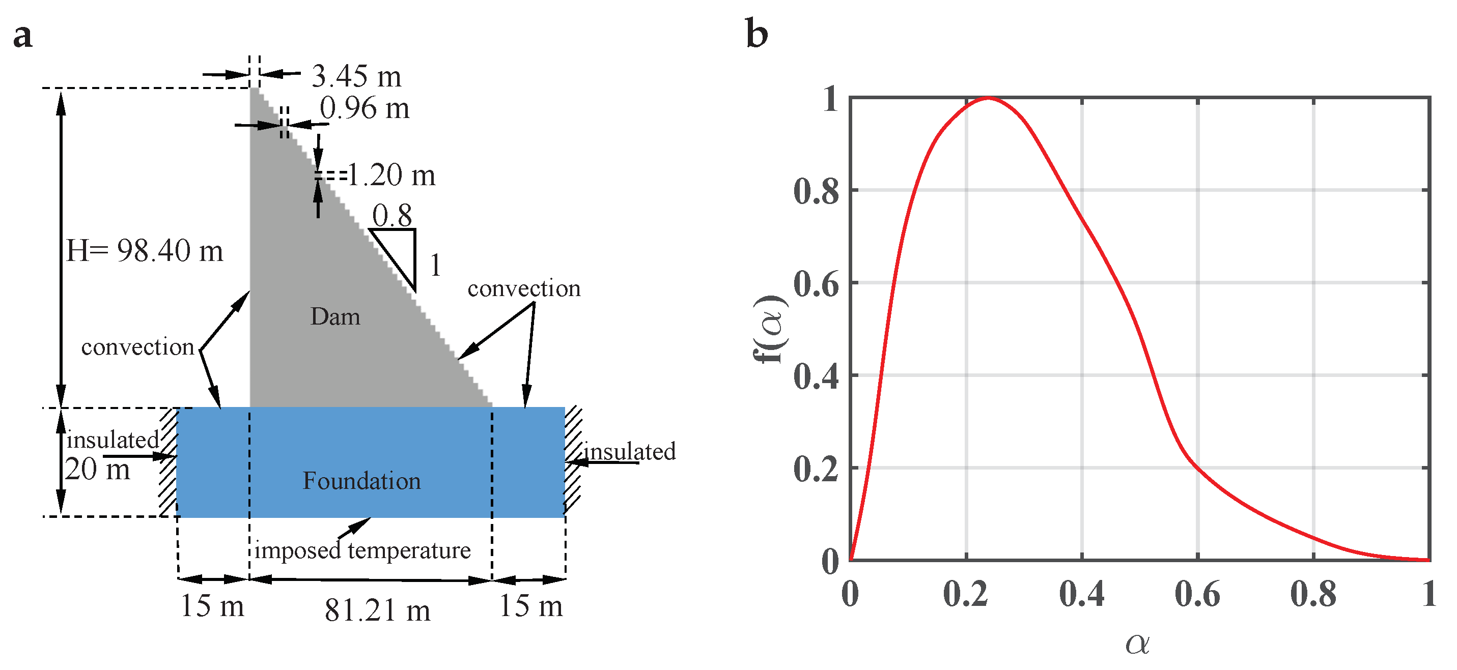
The height of the dam from the foundation to the crest is m; the crest is m in width; the length of the dam at the base is m; and the height and width of the steps are and m respectively. Other dimensions of the dam are included in Figure 1a. We simulate the construction by placing lifts of 30 cm thick every 12 h, at 8 a.m. and 8 p.m. The construction is stopped when the ambient temperature is lower than 2 C or higher than 36 C. Concrete is cooled by replacing part of mixing water by ice. The placing temperature, , is equal to the ambient temperature, , when the latter is between 2 C and 18 C; otherwise, C when is between 18 C and 27 C, and when is between 27 C and 36 C. The concrete curing lasts 14 days, and we simulate it by considering the horizontal surfaces to be humid.
Our domain compromises the dam and a portion of the foundation, Figure 1a. The domain is meshed with squared volumes of size 3 cm. The boundary conditions are: (1) convection at the surfaces in contact with the air at the corresponding equivalent ambient temperature and convection coefficient; (2) no heat flow at the vertical boundaries of the foundation; and (3) imposed temperature at the bottom of the foundation equal to the annual average air temperature. The initial temperature of the foundation is computed with Equation (25). We adopt a time step of 5 min.
The properties of the foundation are: kJ/(mK) and W/(mK). The parameters of the hydration reaction of the concrete are: kJ/(mK), W/(mK), W/m, J/m, and kJ/mol. The normalized heat generation function, , against the degree of hydration, , is represented in Figure 1b. These magnitudes were obtained from laboratory experiments conducted over samples of an RCC dam located in Portugal [24].
We simulated the adiabatic temperature rise with the previous parameters of the NAH for a sample whose initial temperatures were 16 C and 25 C, and we fit the AH exponential model to the simulated data. The best fits were found for s and s, respectively.
4. Results and Discussion
Our methodology is the starting point for the simulation of the thermal evolution in our case study during the construction. The simulations allow us to study the influence of the selection hydration model on the concrete temperature field and on the heat generation rate field. Moreover, the simulation of the hydration reaction with a NAH model lets us study the influence of the environmental actions and the starting date of the construction on the hydration reaction and the concrete temperature evolution.
4.1. Influence of the Hydration Model over the Temperature Field
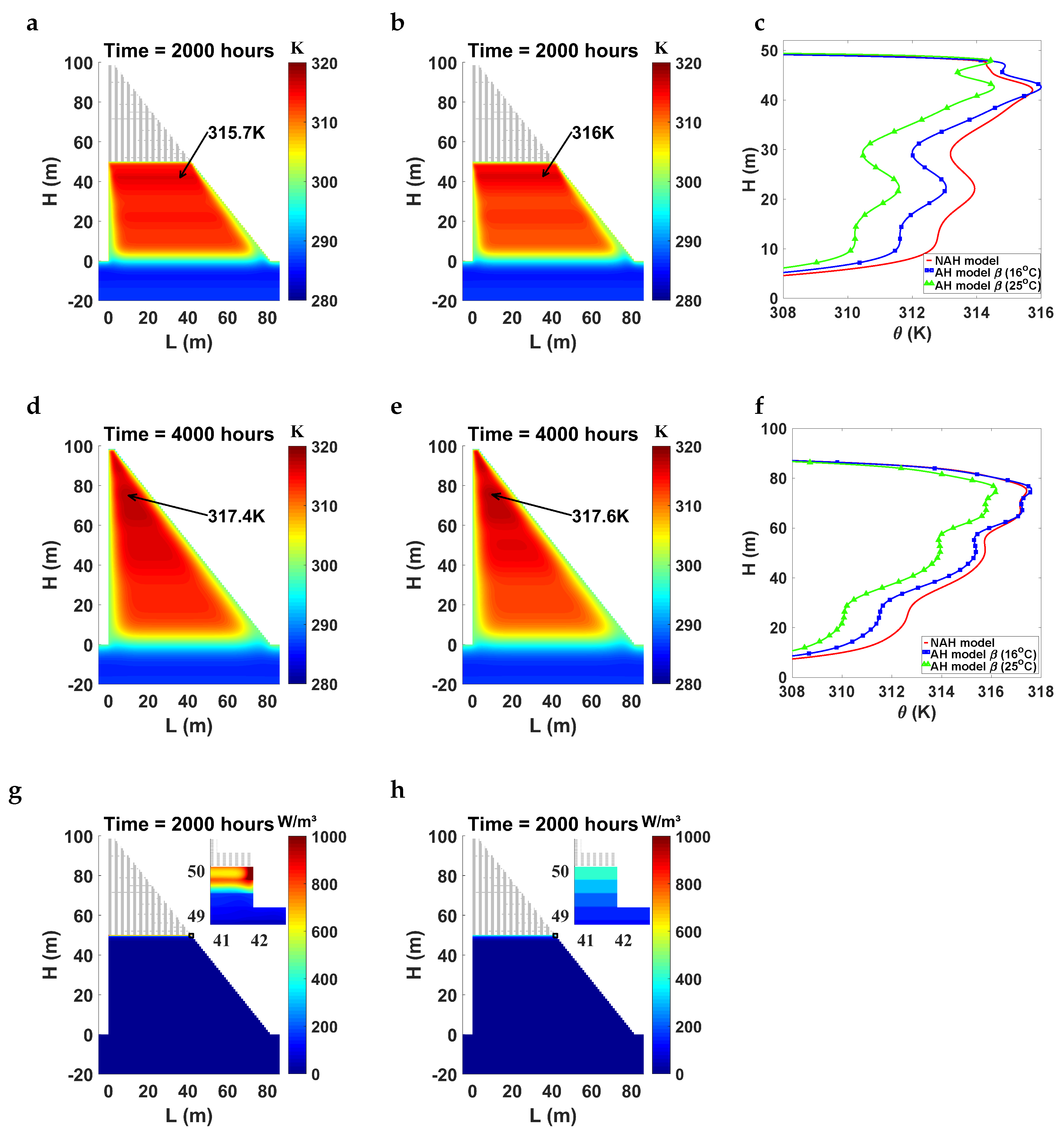
We study the influence of the hydration model on the temperature field by simulating the construction of an RCC dam using three models. The construction starts on 1 April 2014, and lasts 165 days. In the first simulation we adopt a NAH model for the hydration of concrete (first column of Figure 2). In the second simulation we employ an AH model whose -parameter is calibrated for an initial concrete temperature equal to the mean placing temperature, 16 C (second column of Figure 2), and in the third we employ one an AH model with -parameter calibrated for a higher temperature, 25 C. We plot a vertical temperature profile of the dam computed with the three models in the third column of Figure 2.
The temperature fields at mid-height construction time (2000 h) present significant differences between the three simulations. The simulation with the NAH model, Figure 2a, provides higher temperatures in the core of the dam than the ones with the AH model. The NAH model accounts for the effect of the weather conditions on the hydration process, the heat generation rate being higher as the concrete temperature increases. Because the placing temperature of the concrete is relatively low, the generation rate after setting is also low. Then, the hydration reaction slowly evolves for the first 12 h as concrete remains cold because most of the heat is dissipated into the atmosphere. After those 12 h, a new lift is placed and works as a thermal insulation lift; then the temperature of the concrete rises and the heat generation rate also does. As a result, the hydration reaction feeds back itself: as the concrete temperature is higher, the heat generation rate also does and makes the temperature increase.
The simulation with the AH model whose -parameter is calibrated for the mean placing temperature, Figure 2b, provides lower temperatures in the core of the dam than the simulation with the NAH model, Figure 2c. The formulation of the AH model, Equation (4), has the maximum heat generation rate occur at the placing time, i.e., for s, and decrease exponentially with time. Moreover, during the 12 h after pouring concrete, the top surface of the lift is subjected to the environmental actions, and consequently, a significant part of the hydration heat is dissipated into the atmosphere. Furthermore, the relatively low ambient temperature in spring stimulates the dissipation of the heat into the atmosphere.
The simulation with the AH model with the highest -parameter results in lower concrete temperatures in the core of the dam (Figure 2c). The -parameter controls the heat generation rate, and q is higher as the parameter increases. Consequently, more heat is generated for the 12 h after placing, and more heat is dissipated into the environment, resulting in a lower concrete temperature rise.
Once construction has finished (time 4000 h), the core of the dam is hotter than the faces in all the simulations (Figure 2d,e). Nevertheless, the simulation with the NAH model results in higher temperatures than the simulations with the AH model in most parts of the dam; see Figure 2f. The difference accentuates for the AH model with the higher -parameter.
The distribution of the heat generation rate at time 2000 h is highly influenced by the adopted hydration model. The NAH model—Figure 2g—captures the effect of the concrete temperature on the heat generation rate, whereas the AH model does not—Figure 2h—and provides a uniform rate within a given lift. The concrete temperature is also greatly influenced by the environmental actions. At time 2000 h, the last lift was cast at 8 a.m. on June 22, 2014, and the upstream vertical faces were exposed to sunbeams. Therefore, the concrete temperature rises, and the heat generation rate also does, as can be appreciated in the snapshot of Figure 2. The horizontal faces are also exposed to sunbeams, but the evaporation of the curing water cools the concrete and counteracts the effect of the solar radiation.
4.2. Influence of the Weather Conditions on the Evolution of the Hydration Reaction and Concrete Temperature
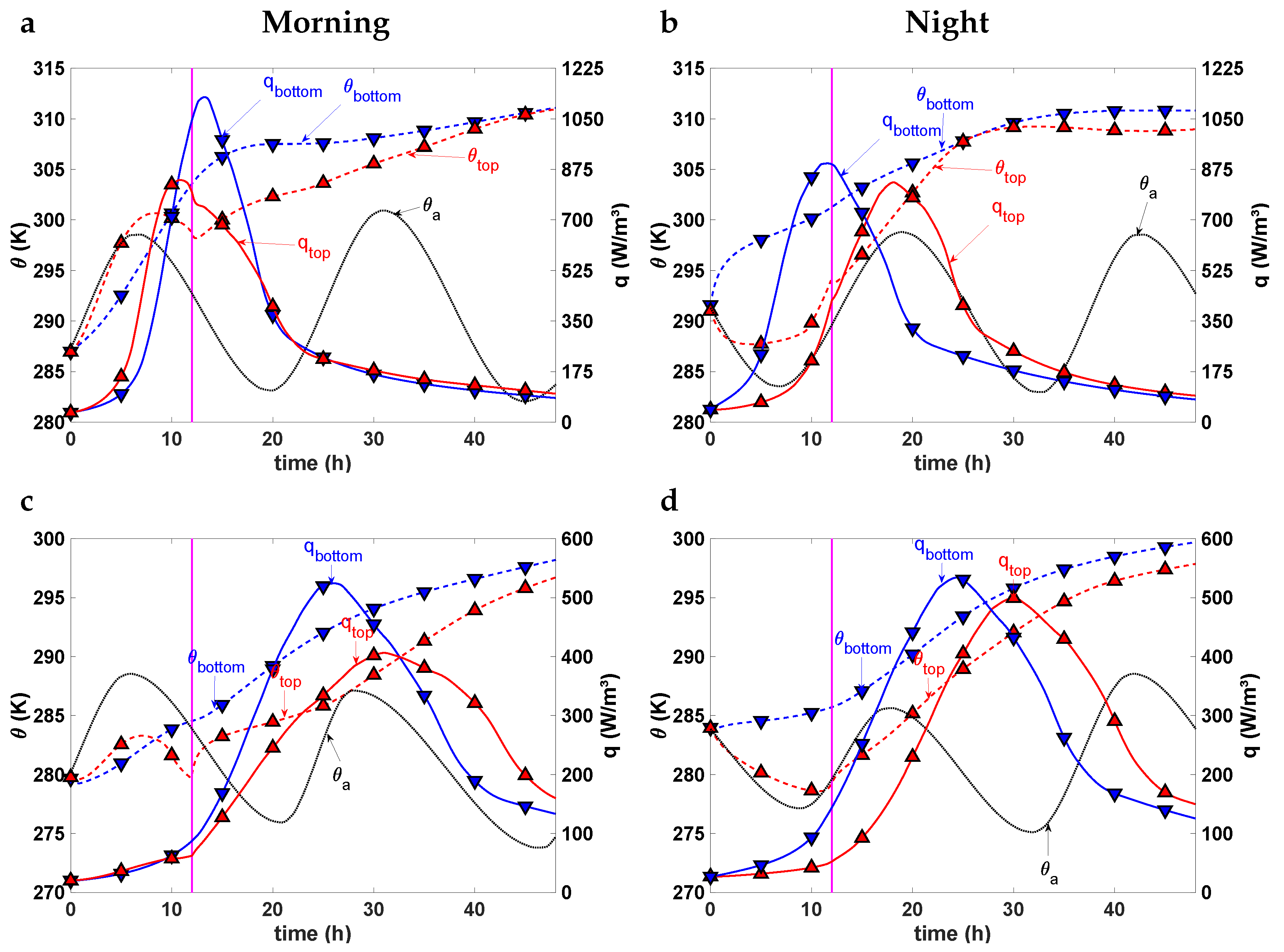
We illustrate the effects of the weather conditions on the evolution of the hydration reaction and the concrete temperature by analyzing the evolution of each variable at several points and under different environmental conditions; see Figure 3. We run two simulations with our case study: in the first one the construction starts on 1 April 2014, and takes place in spring; and in the second simulation it starts on 1 October 2014, and extend s into autumn. We plot the evolutions of several variables at four representative points. Two points are located at the top and the bottom of the lift located at 22.8 m height, which was built on 8 May 2014, at 8 a.m.—in the morning—for the dam built in spring (Figure 3a), and on 7 November 2014, at 8 a.m. for the dam built in autumn (Figure 3c). The other two points are located at the top and bottom of the lift at 21.9 m height, built on 6 May 2014, at 8 p.m.—at night—for the dam construction starting in April, 2014, (Figure 3b), and on 7 November 2014, at 8 a.m. for the dam built in autumn (Figure 3d). The NAH model provides a rich-variety of evolutions of q, in contrast to the AH model, which gives only one evolution. Moreover, q also drives the evolution of , and in turn, the evolution of the mechanical properties.
The evolution of the heat generation rate q—Figure 3—is driven by the environmental conditions and the concrete temperature, , during the first 12 h. During that period, the top surface of the last lift is directly exposed to the weather conditions. Afterward, a new lift is placed and the concrete hydrates under quasi-adiabatic conditions. This situation is not given in those points closed to the dam faces, since concrete hydrates under quasi-isothermal conditions. Several evolution patterns are given, depending on the weather conditions—spring or autumn; casting time of concrete; day or night; and position within the lift, top or bottom.
The heat generation rate for the points of the dam built in spring, cast in the morning, and located in the top of the lift—Figure 3a—evolves following the ambient temperature, . Since q is low during the first five hours, the concrete temperature follows . Afterward, the concrete temperature exceeds the ambient one, as the heat released by the concrete is higher than the heat exchanged with the environment. Nevertheless, the drop in the ambient temperature makes the concrete cool down because the heat released into the environment is more than the generated heat. After 12 h, the next lift is cast and the concrete hydrates under quasi-adiabatic conditions. Although q decreases with time, the concrete temperature increases because the heat does not dissipate into the atmosphere. The evolution of q for the points located in the bottom of the lift is not so influenced by the environmental conditions. The concrete temperature gradually increases with time, since the thermal isolation effect of the mass over the point and the sound weather conditions do not allow the concrete to release all the generated heat.
The evolution of q for the points cast at night—Figure 3b—present a similar evolution to the previous ones. The point in the top follows the ambient temperature: initially decreases due to the low generated heat rate and the decrease in , but afterward the concrete warms thanks to the increase in both q and . This effect is more pronounced for the point in the bottom of the lift due to the thermal isolation of the concrete over it.
The heat generated in the dam built in autumn is also greatly influenced by the weather conditions. The concrete temperature of the points in the top of the lift evolves following the ambient tendency, it increases during the day—Figure 3c—and decreases at night—Figure 3d. Nevertheless, the temperature at the bottom always rises because of the thermal isolation of the concrete. In contrast to the dam built in spring, the heat generation rate is very low during the first 12 h, as the lift is directly exposed to the low ambient temperature that slows down the hydration reaction. Afterward, thanks to the thermal isolation of the new lift, the concrete warms and the reaction accelerates.
4.3. Effect of the Weather Conditions on the q-Peak and Time to Peak
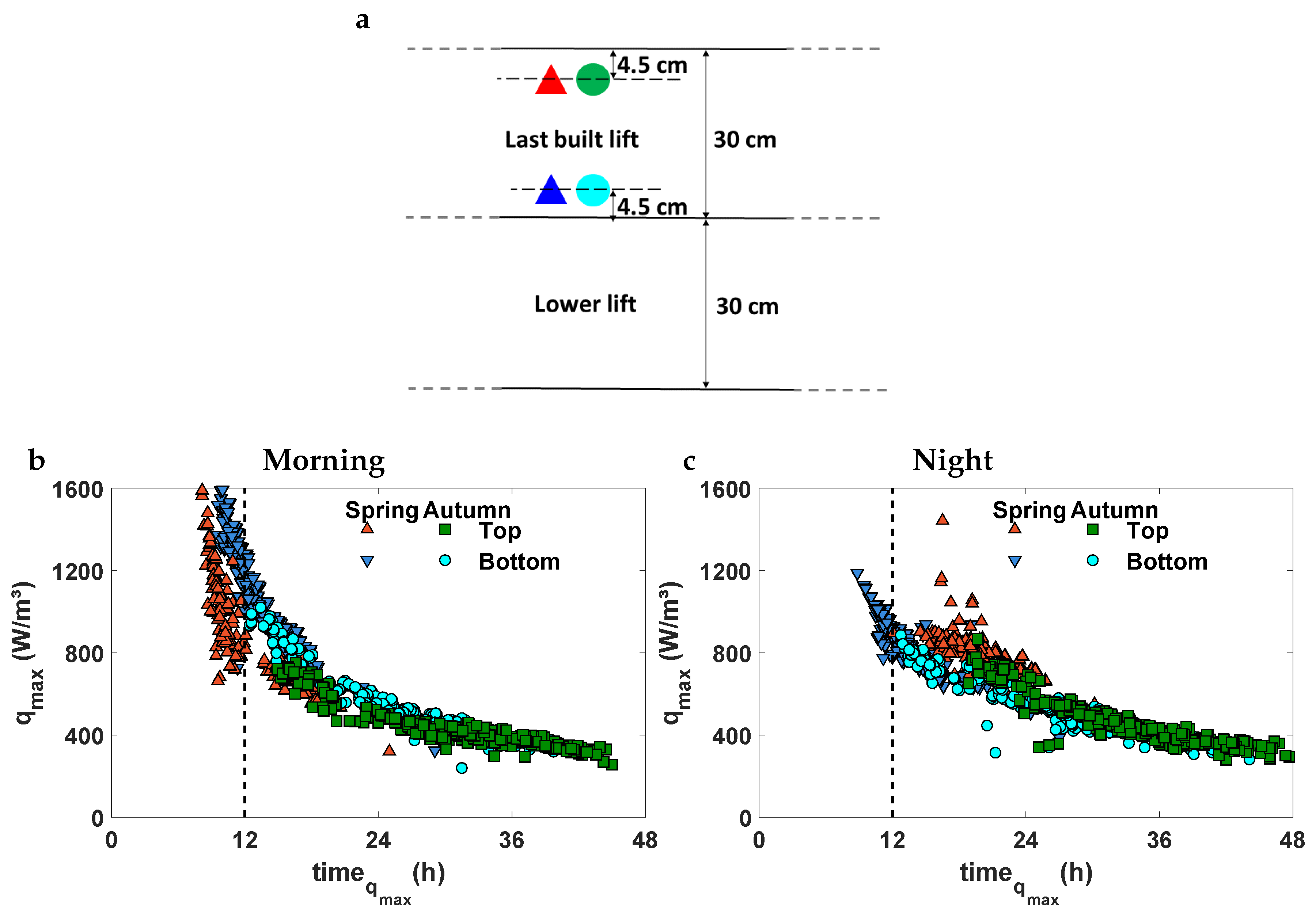
The NAH model provides a rich-variety evolution of q, maximum heat generation rates , and timing of , , in contrast to the AH model, which gives a unique evolution of q. The weather conditions have a direct impact on and , as shown in Figure 4. The lifts cast on spring mornings—Figure 4a—reach higher than the lifts built in autumn. Moreover, most of the peaks in spring are given within the first 12 h after setting the concrete; i.e., before the next lift is built. In contrast, all the peaks in autumn occur after the first 12 h, once the thermal isolation effect of the next lift allows the concrete to warm up.
The lifts set at night present lower values of than those built in the mornings—Figure 4b. The night-time weather conditions make reach lower values. As in the previous case, the lifts built on spring mornings reach higher than the lifts built on autumn mornings. However, the timing of at the top of the lifts delays and peaks is reached after the next lift is cast. Regarding the bottom parts, occurs both before and after casting the next lift in spring, whereas it is given after casting the next lift in autumn.
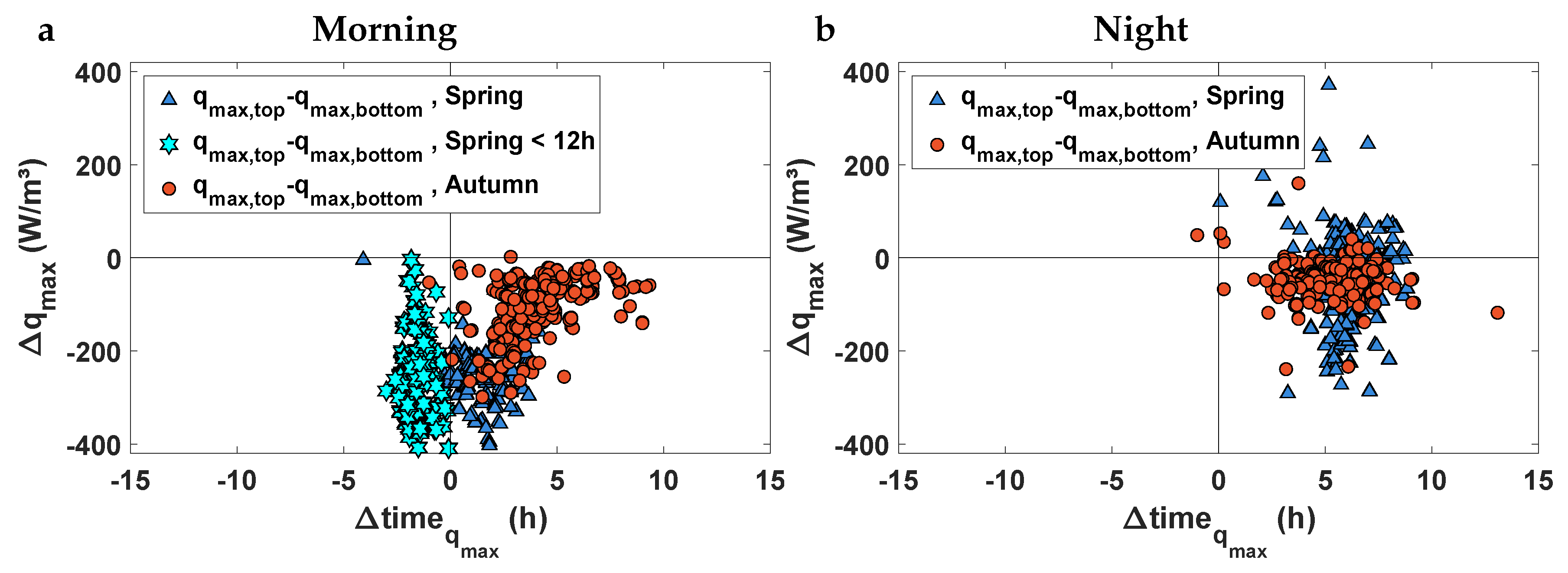
The maximum value of the heat generation rate within every lift for the dam built in spring and lifts placed in the mornings is higher at the bottom than the top—Figure 5a—due to the thermal isolation effect of the top concrete. In the same way, is higher at the top than the bottom—Figure 5a—for those lifts where at the top is lower than 12 h, but is lower at the top than the bottom for those lifts where at the top is higher than 12 h. This behavior comes from the weather conditions: cold days delay the timing of at the top and warm days bring it forward.
The lifts placed at night present a different behavior—Figure 5b. The lifts cast in autumn present in general higher values of and lower at the bottom than at the top. In the case of the lifts disposed in spring, is lower at the bottom than at the top, but no conclusion can be reached regarding .
4.4. Influence of the Boundary Conditions over the Concrete Temperature
We assess the influence of the boundary conditions over the concrete temperature evolution through a new set of simulations. We compute the boundary conditions with a simplified, straightforward methodology that is widely used. The heat exchange between the structure and the environment is boiled down to the convection between the surface of the dam and the air in contact with it. We compare the outputs of several thermal models that incorporate these boundary conditions with the outputs of other models whose boundary conditions are computed with our methodology.
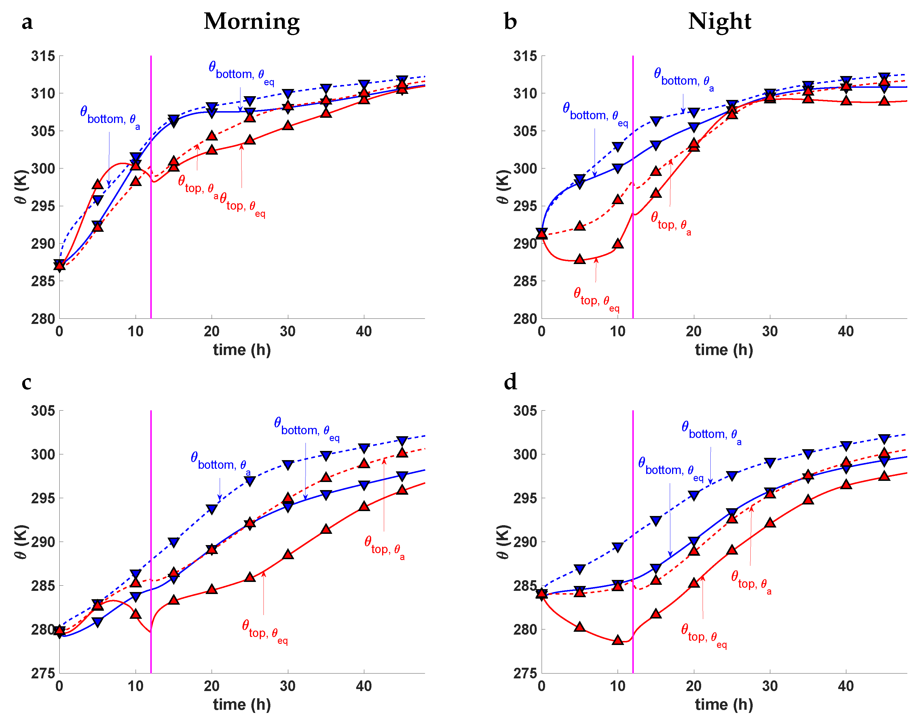
We run two new simulations whose boundary conditions are assessed with the simplified approach: the first simulation corresponds to a dam built in spring, and the second one in autumn. We plot the evolution of the concrete temperature at four representative points. Two points are, respectively, the top and the bottom of the lift at 22.8 m height, built on 8 May 2014, at 8 a.m.—in the morning—of the dam built in spring, Figure 6a; and the same for 7 November 2014, 8 a.m.—the dam built in autumn (Figure 6c). The other two points are located at the top and bottom of the lift at 21.9 m height, built on 6 May 2014, at 8 p.m.—at night—in the dam built in spring, Figure 6b; and the same for 7 November 2014, at 8 a.m.—the dam built in autumn (Figure 6d). We simulate the evolution of with both boundary condition methodologies: our proposal and the simplified methodology.
The evolution of is highly influence by the boundary conditions, especially during the early ages of concrete. In the short term, less than 12 h after casting, both methodologies provide quite different results, whereas in the long term results are similar. Nevertheless, the simplified methodology always results in higher temperature rises. The differences arise from the heat exchange mechanisms: the simplified methodology does not account for the solar radiation, nor the long wave radiation exchange, nor the night cooling effect.
Our methodology provides higher concrete temperatures in the top points cast in the morning of May, Figure 6a, than the outputs provided by the model with the simplified approach. The higher temperature rise is explained by the effect of the solar radiation, which warms the concrete and speeds up the hydration reaction. This effect is not so noticeable in the top point cast in the morning of November, Figure 6c, since solar radiation in autumn is less intense than in spring. Nevertheless, after sunset our model provides lower concrete temperatures than the simplified methodology due to the night cooling effect, which cools down concrete and speeds down the hydration reaction.
The differences in temperatures at the bottom points of the lifts are also noticeable. Since our methodology incorporates the night cooling effect, concrete temperatures on the top surface of the dam are cooler than the outputs provided by the model with the simplified boundary conditions. Once the next lift is cast, the newly poured concrete releases heat to the bottom lift and the hydration reaction speeds down. Consequently, our methodology provides lower temperature rise for the bottom points.
The night cooling has also important effects on the lifts cast at night. The temperature of the top points computed with the model that incorporates our methodology drops at night, whereas the temperature rises in the models with the simplified methodology. This behavior is given in both the dam built in spring, Figure 6b, and the one built in autumn, Figure 6d.
4.5. Effect of the Construction Date on the Thermal Field
The weather conditions during the construction influence the hydration process, and consequently, the temperature field. For this purpose, we simulate the construction of two RCC dams whose constructions start in October, 2014—autumn, and April, 2014—spring, respectively. The construction lasts 165 days for each. We adopt the NAH formulation.
The temperature field for the dam built in spring, Figure 7a,b, is higher or equal at every point compared to the dam built in autumn, Figure 7c,d. Moreover, the hottest areas of the core are in the upper part of the former dam, whereas the hottest areas are in the lower part of the latter one.
In spring, weather becomes warmer with time. As a result, less heat is dissipated, as the placing time is later and concrete temperature after hydration is higher. For this reason, the hottest part of the core is in the upper part of the dam built in spring. Instead, during the fall the weather becomes colder as time advances. The dam is more prone to dissipate heat as the placing time is later. The hottest areas of the core are in the lower part, which was built with warmer weather conditions.
5. Conclusions
We have simulated the thermal evolutions of roller-compacted concrete (RCC) dams under construction. Two important ingredients of our numeral framework are: (1) the heat generation formulation for simulating the hydration reaction of the concrete, and (2) the boundary conditions of the thermal problem.
We have adopted both a non-adiabatic hydration (NAH) model and an adiabatic hydration (AH) model for simulating the hardening of the concrete. The model considers the temperature of the concrete, , and the hydration degree for computing the heat generation rate, q. In contrast, the AH model assumes that concrete hydrates under adiabatic conditions. The evolution of q is only driven by time. Moreover, we have incorporated to the computation of the boundary conditions the following heat flux mechanisms: convection, long wave radiation, solar radiation, and evaporation of water.
Our simulations have shown that the NAH model provides higher temperatures in the concrete than the AH formulation. The AH model assumes that the maximum heat generation rate takes place just after placing the concrete. A large amount of heat is dissipated until the next lift is placed. Then, the new lift works as an thermal insulation and the temperature of the concrete continues rising. In contrast, the simulations with the AH model have evidenced that the hydration reaction is slow after placing the concrete. The concrete progressively warms and q increases. Then, the peak of q does not occur just after placing. Consequently, the amount of heat dissipated before the next lift is placed is, in general, lower than in the simulations with the NAH model.
The weather conditions also affect the hydration reaction. The AH formulation leads to a rich variety of evolutions for q. Both the weather conditions and the insulation provided by the newly placed lifts explain the evolutions. In contrast, the AH model results in a unique evolution for q.
We have adopted a detailed methodology to compute the boundary conditions of the thermal problem. Our methodology captures the main mechanisms that control the heat exchange of the dam with the surroundings. We have compared the outputs of a model with boundary conditions assessed with our methodology with the results of a model with simplified boundary conditions that only account for the convection with the air. In the short term, less than 12 h after casting, our methodology provides higher concrete temperatures in the top points of lifts cast in the mornings due to the solar radiation. Moreover, in the case of top points cast at night, our methodology results in lower temperatures due to the night cooling effect. In the long term, both approaches provide similar temperatures, but our methodology results in slightly lower temperatures compared to the outputs provided by the simplified approach.
We have also confirmed that the starting date of the construction affects both q and . Those dams built in autumn result in lower and delayed peaks for q than those built in spring. Moreover, the temperate field at mid-construction is greater or equivalent at every point for the dams built in spring compared to the ones built in autumn. The position of the hottest area in the core of the dam is also influenced by the weather conditions. The hottest area of those dams built in autumn is located in the lower part of the core, whereas for those built in spring it is in the upper part.
Our simulations have shown that the choice of the hydration model is a key aspect. Results of the thermal simulations may be underestimates if the model is not properly selected. Moreover, our investigation has also illustrated how the weather conditions influence the evolution of the temperature field. Our approach also captures the key controlling mechanisms of the heat exchange between the dam and the surrounding environment and shows promise for simulating and understanding more complex processes in the evolution of the temperatures during the construction of concrete dams.
Author Contributions
Investigation, C.P.-F., D.S., and M.Á.T. All authors have read and agreed to the published version of the manuscript.
Funding
C.P.-F. gratefully acknowledges funding from “Fundación José Entrecanales Ibarra” and “Consejo Social de la Universidad Politécnica de Madrid.”
Acknowledgments
This research was supported by the Ministerio de Economía y Competitividad (Spanish Ministry of Economy and Competitiveness) under grant RTC-2015-3794-5 titled “ACOMBO. Desarrollo de un código de cálculo para el análisis termo-tensodeformacional complejo de las presas bóveda.”
Conflicts of Interest
The authors declare no conflict of interest.
Abbreviations
The following abbreviations are used in this manuscript:
| AH | Adiabatic hydration |
| NAH | Non-adiabatic hydration |
| RCC | Roller-compacted concrete |
References
- U.S. Bureau of Reclamation. Roller-Compacted Concrete: Design and Construction Considerations for Hydraulic Structures; U.S. Dept. of the Interior, Bureau of Reclamation, Technical Service Center: Denver, CO, USA, 2005.
- Cervera, M.; Oliver, J.; Prato, T. Simulation of construction of dams. II: Stress and damage. J. Struct. Eng. 2000, 126, 1062–1069. [Google Scholar] [CrossRef]
- Belmokre, A.; Mihoubi, M.K.; Santillán, D. Analysis of Dam Behavior by Statistical Models: Application of the Random Forest Approach. KSCE J. Civ. Eng. 2019, 23, 4800–4811. [Google Scholar] [CrossRef]
- Santillán, D.; Salete, E.; Toledo, M. A methodology for the assessment of the effect of climate change on the thermal-strain-stress behaviour of structures. Eng. Struct. 2015, 92, 123–141. [Google Scholar] [CrossRef]
- Fourier, J. Theorie Analytique de la Chaleur; Chez Firmin Didot, Père et Fils: Sceaux, France, 1822. [Google Scholar]
- Jaafar, M.; Bayagoob, K.; Noorzaei, J.; Thanoon, W.A. Development of finite element computer code for thermal analysis of roller-compacted concrete dams. Adv. Eng. Softw. 2007, 38, 886–895. [Google Scholar] [CrossRef]
- U.S. Bureau of Reclamation. Cooling of Concrete Dams; U.S. Dept. of the Interior, Bureau of Reclamation, Technical Service Center: Denver, CO, USA, 1949.
- Bofang, Z. Thermal Stresses and Temperature Control of Mass Concrete; Elsevier: Oxford, UK, 2013. [Google Scholar]
- ACI Committee 207. ACI 207.1R-96. Mass Concrete; Technical Report; American Concrete Institute: Farmington Hills, MI, USA, 1997. [Google Scholar]
- ACI Committee 207. ACI 207.2R-95. Effect of Restraint, Volume Change, and Reinforcement on Cracking of Mass Concrete; Technical Report; American Concrete Institute: Farmington Hills, MI, USA, 2002. [Google Scholar]
- Luna, R.; Wu, Y. Simulation of temperature and stress fields during RCC dam construction. J. Constr. Eng. Manag. 2000, 126, 381–388. [Google Scholar] [CrossRef]
- Chen, Y.; Wang, C.; Li, S.; Wang, R.; He, J. Simulation analysis of thermal stress of dams using 3-D finite element relocating mesh method. Adv. Eng. Softw. 2001, 32, 677–682. [Google Scholar] [CrossRef]
- Zhang, X.-F.; Li, S.-Y.; Chen, Y.-L.; Chai, J.-R. The development and verification of relocating mesh method for the computation of temperature field of dam. Adv. Eng. Soft. 2009, 40, 1119–1123. [Google Scholar] [CrossRef]
- Noorzaei, J.; Bayagoob, K.; Thanoon, W.; Jaafar, M. Thermal and stress analysis of Kinta dam. Eng. Struct. 2006, 28, 1795–1802. [Google Scholar] [CrossRef]
- Abdulrazeg, A.; Noorzaei, J.; Mohammed, T.; Jaafar, M. Modeling of combined thermal and mechanical action in roller-compacted concrete dam by three-dimensional finite element method. Struct. Eng. Mech. 2013, 47, 1–25. [Google Scholar] [CrossRef]
- Khanzaei, P.; Abdulrazeg, A.A.; Samali, B.; Ghaedi, K. Thermal and structural response of dams during their service life. J. Therm. Stresses 2015, 38, 591–609. [Google Scholar] [CrossRef]
- Yang, J.; Hu, Y.; Zuo, Z.; Jin, F.; Li, Q. Thermal analysis of mass concrete embedded with double-lift staggered heterogeneous cooling water pipes. Appl. Therm. Eng. 2012, 35, 145–156. [Google Scholar] [CrossRef]
- Reinhardt, H.; Blaauwendraad, J.; Jongedijk, J. Temperature development in concrete structures taking account of state dependent properties. In Proceedings of the RILEM Internatinal Conference on Concrete at Early Ages, Paris, France, 6–8 April 1982; pp. 211–218. [Google Scholar]
- De Schutter, G.; Taerwe, L. General hydration model for portland cement and blast furnace slag cement. Cem. Concr. Res. 1995, 25, 593–604. [Google Scholar] [CrossRef]
- Cervera, M.; Oliver, J.; Prato, T. Simulation of construction of RCC dams. I: Temperature and aging. J. Struct. Eng. 2000, 126, 1053–1061. [Google Scholar] [CrossRef] [Green Version]
- Cervera, M.; García-Soriano, J. Simulación numérica del comportamiento termo-mecánico de presas de HCR Parte I: Modelización y calibración. Revista Internacional de Métodos Numéricos para Cálculo y Diseño en Ingeniería 2001, 17, 491–504. [Google Scholar]
- Cervera, M.; García-Soriano, J. Simulación numérica del comportamiento termo-mecánico de presas de HCR Parte II: Aplicación a la Presa de Rialb. Revista Internacional de Métodos Numéricos para Cálculo y Diseño en Ingeniería 2002, 18, 95–110. [Google Scholar]
- Gaspar, A.; Lopez-Caballero, F.; Modaressi-Farahmand-Razavi, A.; Gomes-Correia, A. Methodology for a probabilistic analysis of an RCC gravity dam construction. Modelling of temperature, hydration degree and ageing degree fields. Eng. Struct. 2014, 65, 99–110. [Google Scholar] [CrossRef]
- Azenha, M. Numerical Simulation of the Structural Behaviour of Concrete since Its Early Ages. Ph.D. Thesis, University of Porto, Porto, Portugal, 2009. [Google Scholar]
- Faria, R.; Azenha, M.; Figueiras, J.A. Modelling of concrete at early ages: Application to an externally restrained slab. Cem. Concr. Compos. 2006, 28, 572–585. [Google Scholar] [CrossRef]
- Azenha, M.; Faria, R. Temperatures and stresses due to cement hydration on the r/c foundation of a wind tower—A case study. Eng. Struct. 2008, 30, 2392–2400. [Google Scholar] [CrossRef]
- Azenha, M.; Faria, R.; Ferreira, D. Identification of early-age concrete temperatures and strains: Monitoring and numerical simulation. Cem. Concr. Compos. 2009, 31, 369–378. [Google Scholar] [CrossRef]
- Santillán, D.; Salete, E.; Vicente, D.; Toledo, M. Treatment of solar radiation by spatial and temporal discretization for modeling the thermal response of arch dams. J. Eng. Mech. 2014, 140, 05014001. [Google Scholar] [CrossRef]
- Santillán, D.; Salete, E.; Toledo, M.; Granados, A. An improved 1D-model for computing the thermal behaviour of concrete dams during operation. Comparison with other approaches. Comput. Concr. 2015, 15, 103–126. [Google Scholar] [CrossRef]
- Santillán, D.; Salete, E.; Toledo, M. A new 1D analytical model for computing the thermal field of concrete dams due to the environmental actions. Appl. Therm. Eng. 2015, 85, 160–171. [Google Scholar] [CrossRef]
- Chen, H.; Liu, Z. Temperature control and thermal-induced stress field analysis of GongGuoQiao RCC dam. J. Therm. Anal. Calorim. 2019, 135, 2019–2029. [Google Scholar] [CrossRef]
- Alembagheri, M. A Study on Structural Safety of Concrete Arch Dams During Construction and Operation Phases. Geotech. Geol. Eng. 2019, 37, 571–591. [Google Scholar] [CrossRef]
- Salete, E.; Lancha, J.C. Presas de Hormigión. Problemas Térmicos Evolutivos; Colección Seinor, 18; Colegio de Ingenierios de Caminos, Canales y Puertos: Madrid, Spain, 1998. [Google Scholar]
- Van Breugel, K. Simulation of Hydration and Formation of Structure in Hardening Cement-Based Materials. Ph.D. Thesis, Delft University of Technology, Delft, The Netherlands, 1991. [Google Scholar]
- De Schutter, G.; Taerwe, L. Specific heat and thermal diffusivity of hardening concrete. Mag. Concr. Res. 1995, 47, 203–208. [Google Scholar] [CrossRef]
- Kehlbeck, F. Einfluss der Sonnenstrahlung bei Brückenbauwerken; Werner-Verlag: Düsseldorf, Germany, 1975. [Google Scholar]
- Branco, F.; Mendes, P.; Mirambell, E. Heat of hydration effects in concrete structures. ACI Mater. J. 1992, 89, 139–145. [Google Scholar]
- Chen, B.; Clark, D.; Maloney, J.; Mei, W.; Kasher, J. Measurement of night sky emissivity in determining radiant cooling from cool storage roofs and roof ponds. In Proceedings of the National Passive Solar Conference, Minneapolis, MN, USA, 15–20 July 1995; Volume 20, pp. 310–313. [Google Scholar]
- Lawrence, M. The relationship between relative humidity and the dewpoint temperature in moist air: A simple conversion and applications. Bull. Am. Meteorol. Soc. 2005, 86, 225–233. [Google Scholar] [CrossRef]
- Reindl, D.; Beckman, W.; Duffie, J. Diffuse fraction correlations. Sol. Energy 1990, 45, 1–7. [Google Scholar] [CrossRef]
- Chuntranuluck, S.; Wells, C.; Cleland, A. Prediction of chilling times of foods in situations where evaporative cooling is significant—Part 1. Method development. J. Food Eng. 1998, 37, 111–125. [Google Scholar] [CrossRef]
- Kusuda, T.; Achenbach, P.R. Earth Temperature and Thermal Diffusivity at Selected Stations in the United States; Technical Report; National Bureau of Standards: Washington, DC, USA, 1965.
- Miehe, C.; Hofacker, M.; Welschinger, F. A phase field model for rate-independent crack propagation: Robust algorithmic implementation based on operator splits. Comput. Methods Appl. Mech. Eng. 2010, 199, 2765–2778. [Google Scholar] [CrossRef]
- Santillán, D.; Mosquera, J.C.; Cueto-Felgueroso, L. Phase-field model for brittle fracture. Validation with experimental results and extension to dam engineering problems. Eng. Fract. Mech. 2017, 178, 109–125. [Google Scholar] [CrossRef]
- Santillán, D.; Mosquera, J.C.; Cueto-Felgueroso, L. Fluid-driven fracture propagation in heterogeneous medium: Probability distributions of fracture trajectories. Phys. Rev. E 2017, 96, 053002. [Google Scholar] [CrossRef] [PubMed]
- Santillán, D.; Juanes, R.; Cueto-Felgueroso, L. Phase field model of hydraulic fracturing in poroelastic media: Fracture propagation, arrest and branching under fluid injection and extraction. J. Geophys. Res. Solid Earth 2017, 123, 2127–2155. [Google Scholar] [CrossRef]
- Santillán, D.; Juanes, R.; Cueto-Felgueroso, L. Phase field model of fluid-driven fracture in elastic media: Immersed-fracture formulation and validation with analytical solutions. J. Geophys. Res. Solid Earth 2017, 122, 2565–2589. [Google Scholar] [CrossRef] [Green Version]
- Fritsch, F.N.; Carlson, R.E. Monotone piecewise cubic interpolation. SIAM J. Numer. Anal. 1980, 17, 238–246. [Google Scholar] [CrossRef]
Figure 1.
Illustration of the case study and properties of the concrete. (a) We simulate the thermal evolution of a roller-compacted concrete (RCC) dam during the construction phase. The boundaries of our numerical model are: (1) convection at the surfaces in contact with the air at the corresponding equivalent temperature, (2) no heat flow at the vertical boundaries of the foundation, and (3) imposed temperature at the bottom of the foundation. In the same figure, we also include the dimensions of our model. (b) Here we plot the normalized heat generation function, , against the degree of hydration, , of concrete.

Figure 2.
Influence of the hydration model on the temperature field. The construction of the dam begins on 1 April 2014, and lasts 165 days. We simulate the evolution of the temperature field using a NAH model, and two AH models with -parameters equal to s and s, which correspond to placing temperatures of 16 C and 25 C respectively. We depict the temperature fields when the construction is at mid-height (50 m) (a) for the NAH model, and (b) for the AH model with s. We compare the temperature fields in a vertical profile located 10 m from the upstream face for the three simulations (c). We repeat the three plots when the construction has finished in panels (d)–(f). The heat generation rate at mid-height time computed with the NAH model is included in the panel (g), and the AH model with s is in panel (h). We also include a view of the last five lifts built in the insets.

Figure 3.
Here we illustrate the influence of the weather conditions on the heat hydration. We have simulated the construction of an RCC dam starting at two different times: on 1 April 2014, (first row), and 1 October 2014, (second row). The construction processes last 165 days and take place in spring and autumn, respectively. The evolution of the concrete temperature is represented by the dashed lines, the heat generation rate by the solid lines, and the ambient temperature by the dotted line. Red lines represent the evolution of points situated at the top of the considered lift, and blue lines—those at the bottom. Panel (a) includes the evolution of the points situated in the lift at 22.8 m height and built on 8 May 2014, at 8 a.m.—spring morning; and panel (b) represents sparse points of the lift at 21.9 m height and built on 6 May 2014, at 8 p.m.—spring night. Similar results are presented for the dam construction starting on October, 2014; panel (c) depicts the evolutions of the points in lift at 22.8 m height and built on 7 November 2014, at 8 a.m.—autumn morning. (d) The points in the lift at 21.9 m height and built on 5 November 2014, at 8 p.m.—autumn night.

Figure 4.
Effect of the weather conditions on the maximum heat generation rate, , and timing of , . We have simulated the construction of two RCC dams whose building started in October, 2014—autumn—and April, 2014—spring. The hydration reaction is computed with the NAH model. (a) Here we depict the schematic position of the analyzed points within the lift. (b) We plot against for all the points within the dam body; i.e., points further than 1 m from the lateral dam faces. We set lifts at 8 a.m.; i.e., in the morning. The results of the dam built in spring are represented by triangles; red color depicts the point at the top of the lift, and blue the bottom. The results of the dam cast in autumn are plotted with circles; green color represents point at the top of the lift, and cyan the bottom. (c) Here we depict against time for all points within the dam body and set lifts at 8 p.m.; i.e., at night.

Figure 5.
Here we plot the difference between at the top part of the lift and at the bottom part, , against the difference between at the top part of the lift and at the bottom part, . We plot in panel (a) the results of the lifts set in the morning, and in panel (b) those set at night.
Figure 5.
Here we plot the difference between at the top part of the lift and at the bottom part, , against the difference between at the top part of the lift and at the bottom part, . We plot in panel (a) the results of the lifts set in the morning, and in panel (b) those set at night.

Figure 6.
Here we illustrate the influence of the boundary conditions over the evolution of the concrete temperature. We have simulated the construction of a RCC dam starting on 1 April 2014, (first row), or 1 October 2014, (second row). The construction lasts 165 days and takes place in spring or autumn, respectively. The boundary conditions of our numerical models are computed through two approaches: (1) the methodology proposed in this paper, and (2) a simplified approach which only accounts for the convection between the dam surface and the air in contact with it. We compute the evolution of the concrete temperature through these two approaches: continuous lines plot the outputs of the models whose boundary conditions are computed with our methodology, and dashed lines with the simplified approach. Red lines represent the evolutions of points situated at the top of the considered lift, and blue lines the bottom. Panel (a) includes the evolution of the points situated in the lift at 22.8 m height and cast on 8 May 2014, at 8 a.m.—spring morning, and panel (b) represents sparse points of the lift at 21.9 m height and cast on 6 May 2014, at 8 p.m.—spring night. Similar results are presented for the dam construction starting in October; panel (c) depicts the evolutions of the points in lift at 22.8 m height and cast on 7 November 2014, at 8 a.m.—autumn day, and panel (d) the points in the lift at 21.9 m height and cast on 5 November 2014, at 8 p.m.—autumn night.

Figure 7.
Here we illustrate the influences of the construction start date and the hydration model. We have simulated the construction of two RCC dams starting on April, 2014—spring, and October, 2014—autumn. The hydration reaction is computed with the NAH model. We plot the thermal field of the dam built in spring at mid-height in panel (a) and that at the end of the construction in panel (b). The thermal field of the dam built in autumn at mid-height is depicted in panel (c) and that at the end of construction in panel (d).

© 2020 by the authors. Licensee MDPI, Basel, Switzerland. This article is an open access article distributed under the terms and conditions of the Creative Commons Attribution (CC BY) license (http://creativecommons.org/licenses/by/4.0/).
Share and Cite
MDPI and ACS Style
Ponce-Farfán, C.; Santillán, D.; Toledo, M.Á. Thermal Simulation of Rolled Concrete Dams: Influence of the Hydration Model and the Environmental Actions on the Thermal Field. Water 2020, 12, 858. https://doi.org/10.3390/w12030858
AMA Style
Ponce-Farfán C, Santillán D, Toledo MÁ. Thermal Simulation of Rolled Concrete Dams: Influence of the Hydration Model and the Environmental Actions on the Thermal Field. Water. 2020; 12(3):858. https://doi.org/10.3390/w12030858
Chicago/Turabian StylePonce-Farfán, Cristian, David Santillán, and Miguel Á. Toledo. 2020. "Thermal Simulation of Rolled Concrete Dams: Influence of the Hydration Model and the Environmental Actions on the Thermal Field" Water 12, no. 3: 858. https://doi.org/10.3390/w12030858
Note that from the first issue of 2016, this journal uses article numbers instead of page numbers. See further details here.