Seasonal and Diurnal Variations in the Priestley–Taylor Coefficient for a Large Ephemeral Lake


1
Nanjing Institute of Geography and Limnology, Chinese Academy of Sciences, Nanjing 210008, China
2
Key Laboratory of Watershed Geographic Sciences, Chinese Academy of Sciences, Nanjing 210008, China
3
School of Earth Science and Engineering, Hohai University, Nanjing 210098, China
4
Hydrological Bureau of Jingdezhen City, Jingdezhen 333003, China
5
Hydrological Bureau of Poyang Lake, Jiujiang 332800, China
*
Author to whom correspondence should be addressed.
Water 2020, 12(3), 849; https://doi.org/10.3390/w12030849
Submission received: 27 January 2020
/
Revised: 6 March 2020
/
Accepted: 10 March 2020
/
Published: 17 March 2020
(This article belongs to the Section Hydrology)
Abstract
:The Priestley–Taylor equation (PTE) is widely used with its sole parameter (α) set as 1.26 for estimating the evapotranspiration (ET) of water bodies. However, variations in α may be large for ephemeral lakes. Poyang Lake, which is the largest freshwater lake in China, is water-covered and wetland-covered during its high-water and low-water periods, respectively, over a year. This paper examines the seasonal and diurnal variations in α using eddy covariance observation data for Poyang Lake. The results show that α = 1.26 is overall feasible for both periods at daily and subdaily scales. No obvious seasonal trend was observed, although the standard deviation in α for the wetland was larger than that for the water surface. The mean bias in evaporation estimations using the PTE was less than 5 W·m−2 during both periods, and the root mean square errors were much smaller than the average evaporation measurements at daily scale. U-shaped diurnal patterns of α were found during both periods, due partly to the negative correlation between α and the available energy (A). Compared to the vapor pressure deficit (VPD), wind speed (u) exerts a larger contribution to these variations. In addition, u is positively correlated with α during both periods, however, VPD was positively and negatively correlated with α during the high-water and low-water periods, respectively. Subdaily α exhibited contrasting clusters in the (u, VPD) plane under the same available energy ranges. Our study highlights the seasonal and diurnal course of α and suggests the careful use of PTE at subdaily scales.
1. Introduction
Inland water bodies cover less than 4% of the total terrestrial land [1]. However, they exert huge impacts on the terrestrial water cycle, energy cycle, and climate system [2,3,4] because of their higher heat capacity and lower albedo compared to the land surface [5,6]. Understanding the evaporative process of inland waters is therefore important for the application of numerical atmospheric models [7,8,9], especially in regions with large lakes [4]. There are 122 large lakes (>1000 km2) across the globe [10], 10 of which are located in China. Poyang Lake is the largest freshwater lake (3680 km2) in China. The surrounding area of Poyang Lake serves as an important food production base for approximately 10 million people [11]. However, due to hydrological droughts, Poyang Lake’s surface area has decreased in the past three decades [12], which may have great negative impacts on the regional economy and natural ecosystem.
The evapotranspiration (ET) rates of water bodies can be estimated using the humidity gradient between the water surface and the ambient air [13,14]. However, the transfer coefficients at the lake–air interface differ greatly depending on the size, depth, location, and surrounding conditions of the lake [15,16,17]. Since the pioneering work of Priestley and Taylor [18], the evaporation of water bodies has been understood by the surface energy balance, that is, ET = , where A is the available energy flux, and Δ and γ are functions of the air temperature and atmospheric pressure, respectively. The parameter α is determined as 1.26 by regressions using ET and meteorological measurements from large water bodies [18]. Furthermore, analytical considerations indicate that α is approximately 1.26 if the land surface is saturated [19,20].
The Priestley–Taylor (PT) equation is widely used in estimating the ET of water bodies with the α value taken as 1.26 [21,22]. However, numerous studies showed that α can vary from its recommended value. For example, Guo et al. [23] found that an α value of 1.26 led to overestimates of evaporation when H (sensible heat flux) > 0 and LE (latent heat flux) > 0, and underestimates when H < 0 and LE > 0, in a reservoir in Mississippi, USA. Moreover, at subdaily scales, the α of water bodies was found to be correlated with the relative transport efficiency of turbulent heat/vapor [24]. In addition, a 1.26 value for α may result in overall positive biases in estimating the ET of wetlands [25]. Drexler, Snyder [26] also confirmed that α needs local calibration in wetland ET estimation.
Poyang Lake experiences substantial changes in its water level throughout the year (~8–20 m). The bottom land of the lake is covered by water during the high-water period and by mudflats with short grass during the low-water period. A previous study [27] showed that diurnal ET variation is coupled with net radiation (Rn) during the wetland-covered period, but is out of phase with Rn during the water-covered period in Poyang Lake, indicating that diurnal α may experience substantial variations during the water-covered period. As reported in previous studies [23,24], α can be larger than 2 and smaller than 0.5. In addition, the driving forces of ET differ under water-covered and wetland-covered conditions across different temporal scales [28]. In this paper, we study the seasonal and diurnal variations in α and explore their controlling factors in Poyang Lake. Although many studies have discussed the variations in α over water bodies or wetlands, few studies have compared the α variations between water bodies and wetlands. The substantial changes in the water level in Poyang Lake (~8–20 m) provide natural experimentation settings for studying the variations in α and their controlling factors under changing surface conditions. Whether the same value of α is feasible for both water bodies and wetlands and whether the same factors control the variations in α are the main topics of this paper.
2. Background and General Definitions
In a closed system, evaporation from the water’s surface will eventually make the air above the surface saturated (the vapor pressure deficit equals zero). Evaporation is considered equilibrium evaporation (Eeq) under such saturated conditions. Eeq can be theoretically determined as the available energy flux (A) times Δ/(Δ+γ) because the Bowen ratio (B = H/LE) equals γ/Δ in this case, where Δ is the slope of the saturated vapor pressure to the air temperature and γ is the psychrometric constant. Δ and γ are the functions of air temperature and air pressure, respectively. The actual evaporation from wide water surfaces and wetlands is estimated using the concept of equilibrium evaporation and the coefficient α to account for the effect of the drying power of the air on evaporation (Equation (1)). Because A equals Rn − G, α is, therefore, written as Equation (2), where EF is the evaporative fraction (EF = LE/(H + LE)). EF is assumed to be insensitive to wind speed in equilibrium conditions due to the similarity of evaporation and heat conduction [29,30]. The surface heat flux (G) is the heat flux that is conducted from the surface into the water (or from water body to the surface). Due to the high heat capacity of the water body [5,6], the G of lake systems usually takes up a large proportion of the surface energy balance [31,32,33].
Note that Penman [34] derived the evaporation equation (Equation (3)) for water bodies by combining the considerations of the surface energy balance and the heat transfer process (Equation (3)). The first term of Equation (3) is theoretically equal to equilibrium evaporation, and the second term accounts for the effect of the drying power of the air (Ea), which is estimated by the product of the vapor pressure deficit and a function of wind speed. γ/(Δ+γ) represents the fraction of the drying power that transfers into latent heat flux. When the vapor pressure deficit tends to be zero, Equation (3) tends to be Eeq.
Therefore, theoretically, the α of water bodies is correlated with meteorological factors. For example, α increases with an increase in wind speed or the vapor pressure deficit due to the increase of Ea if the available energy flux remains constant. Similarly, α decreases with an increase of the available energy flux if the other factors remain constant.
3. Data and Processing
3.1. Site Description
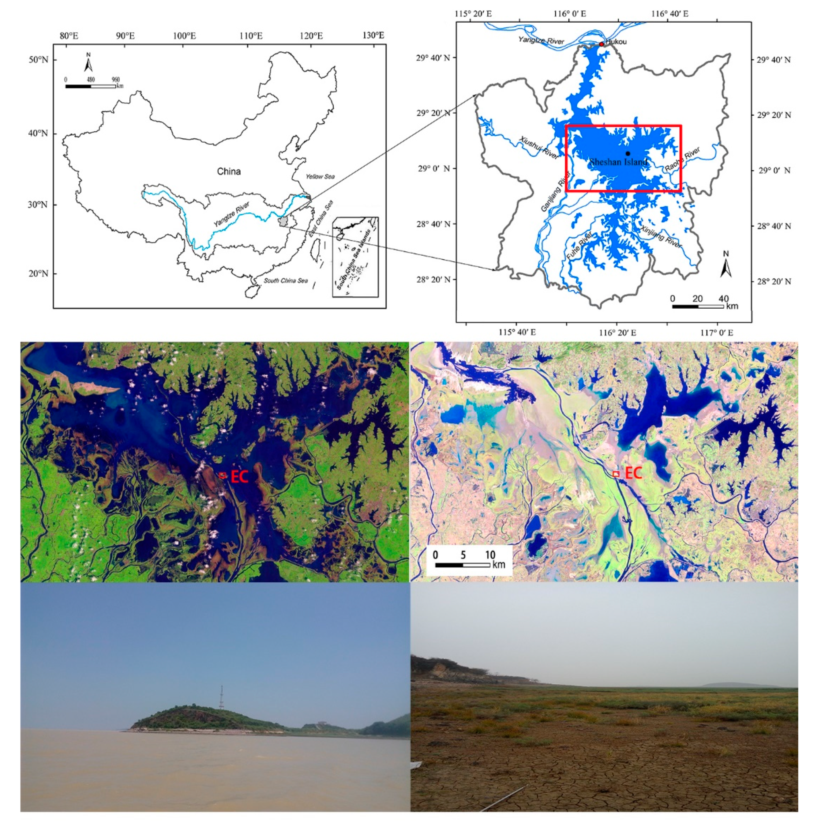
Poyang Lake (28°22′–29°45′ N, 115°47′–116°45′ E) is located on the south bank of the Yangtze River. The Poyang Lake basin has a humid subtropical climate with an annual mean air temperature of 17.5 °C and a multiyear mean precipitation of 1635.9 mm for 1960–2010. Five rivers (Xiushui, Ganjiang, Fuhe, Xinjiang, and Raohe) are the main water suppliers to the lake [35], and the lake discharges to the Yangtze River at Hukou (Figure 1). Poyang Lake has an average depth of 8 m with a high degree of seasonal variation [11]. The inundated area varies remarkably from more than 3000 km2 in summer to less than 1000 km2 in winter [35,36]. The major river routes are covered by water throughout the year, whereas most of the lake basin is only covered by water during the high-water period. The lake periodically reveals its bottom surfaces (i.e., mudflat, grassland, etc.), during the low-water period. The measuring system in this study was set in a periodically inundated zone of Poyang Lake, which changes from a water surface to a wetland periodically within a year.
The high-water period of Poyang Lake normally extends from April to October. Xingzi station is the best site for representing the overall water level (based on the Wusong elevation datum) status of Poyang Lake [37]. The high-water and low-water periods (See Figure in Section 3) for the EC (eddy covariance) site used in this study reveal the times when the water levels at Xingzi station were higher than 14 m, and lower than 12 m, respectively, according to the study that quantified the relationship between the water surface areas of the Poyang Lake and the water level at the Xingzi station [38]. The times when the water levels are within the range of 12–14 m are defined as the transition period. The water level data of Xingzi station were acquired from the Hydrological Bureau of Jiangxi Province (http://www.jxssw.gov.cn/).
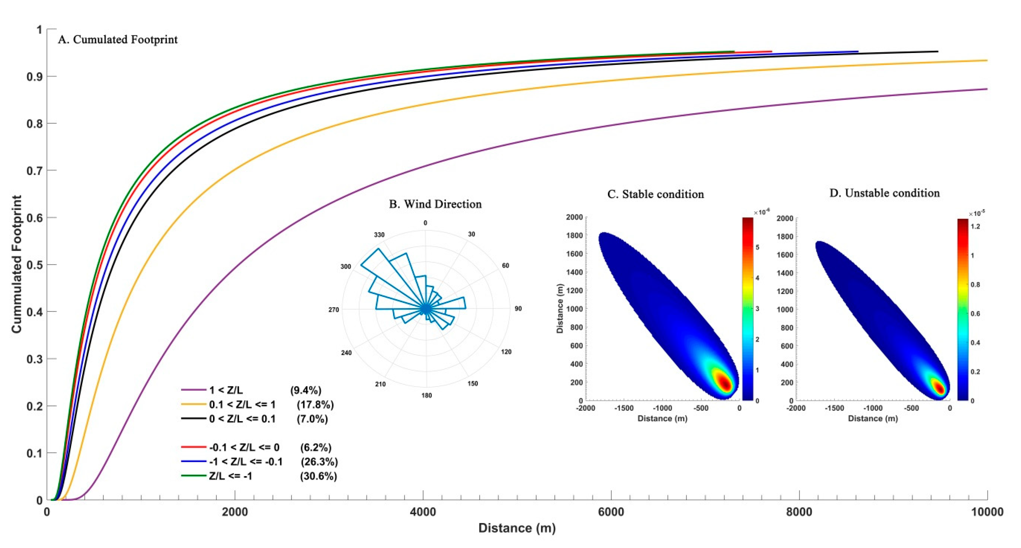
The sensible and latent heat fluxes of the lake were measured by eddy covariance devices from a 38 m tower (29.09° N, 116.38° E) on Sheshan Island, which is located at the center of Poyang Lake (Figure 1). The EC system measures fluxes from the effective upwind source, which can be determined by a footprint analysis of the relative contributions of the flux at each point (x,y) to the EC site (x0,y0). A footprint analysis using the Kljun model [39,40] reveals that the major source area (85%) was within 1~2 km of the wind direction under unstable conditions. Compared to unstable conditions, the extent of the 85% source area was larger under stable conditions. However, the major source area was still within 6 km in most cases except when the surface layer was extremely stable (Zm/L0 > 1, Zm is the measuring height and L0 is the Monin–Obukhov length). Data were discarded when Zm/L0 > 1. Due to the relatively small area of the island (less than 1 km2), the flux contribution from Sheshan Island can be ignored because it is usually small, less than 5% from the major northwest winds (Figure 2B). The water coverage fractions within the EC footprints were generally larger than 90% and smaller than 20% during the high-water and low-water periods, respectively [27]. The data used in this paper are deposited in a public domain repository (https://figshare.com/articles/data_water-12-00849/11968551).
3.2. Data Processing
Turbulences in the air temperature, humidity, and three-dimensional wind velocity were measured by a CO2/H2O analyzer and a 3-D Sonic Anemometer (EC150, Campbell Scientific Inc., Logan, UT, USA). The eddy covariance technique and subsequent corrections were then used to estimate the 30 min scale H and LE using the high-frequency measurements of departures from the mean values. H and LE were calculated using the following equations (Equation (4) and Equation (5)):
where ρ is the dry air density (kg·m−3), cp is the specific heat of dry air (J·g−1·K−1), and λ is the latent heat of vaporization (J·g−1), which is dependent on the air temperature. w′, T′, and q′ are the deviations from the time-averaged vertical wind velocity (m·s−1), air temperature (K), and water vapor density (g·m−3), respectively. In addition, the meteorological forcings were measured at a 30 min scale. The surface radiation components, including the downward/upward short-wave and long-wave radiations, were measured by the pyrgeometers/pyranometers (CNR4, Kipp & Zonen B.V., Delft, The Netherlands). The air temperature and relative humidity were measured by an HMP155A (Vaisala, Helsinki, Finland).
We handled the half-hourly flux measurements using the spike detection technique [41]. The half-hourly data at the timings when the downward shortwave radiation was larger than zero were chosen for diurnal analysis. We also averaged the chosen 30 min scale data for each day to analyze the seasonal variations in α. Overall, we analyzed the variations in α and their controlling factors at two temporal scales—subdaily (diurnal variations) and daily (seasonal variations)—in both the high-water and low-water periods. Because of the large uncertainty in determining G for the water surface, the available energy was surrogated by the sum of the measured H and LE. Because evaporation is mainly controlled by the energy input and aerodynamic transport of water vapor, we chose two categories of controlling factor candidates of α in this study: first, the available energy that drives the land–atmosphere energy transfer process and second, the factors that reflect the evaporative demand of the air and local advection, that is, the wind speed (u) and water vapor pressure deficit of the air (VPD).
We used the stepwise regression method to explore the first-order controlling factors of α. Stepwise regression is a systematic method for constructing an explanatory multilinear model. It adds or removes one of the predictive terms (x1, x2, …, xi, …, xn) from the model at each step based on the statistical significance of the term in the regression. Pcoeff is the p-value of the estimated coefficient of a candidate term xi. A potential predicted term is accepted in the final regression model (status set as ′′In′′) if Pcoeff and PF are smaller than the threshold of 0.05. The stepwise analysis was conducted using MATLAB 2015b.
4. Results and Discussion
4.1. Environmental Conditions and Energy Fluxes
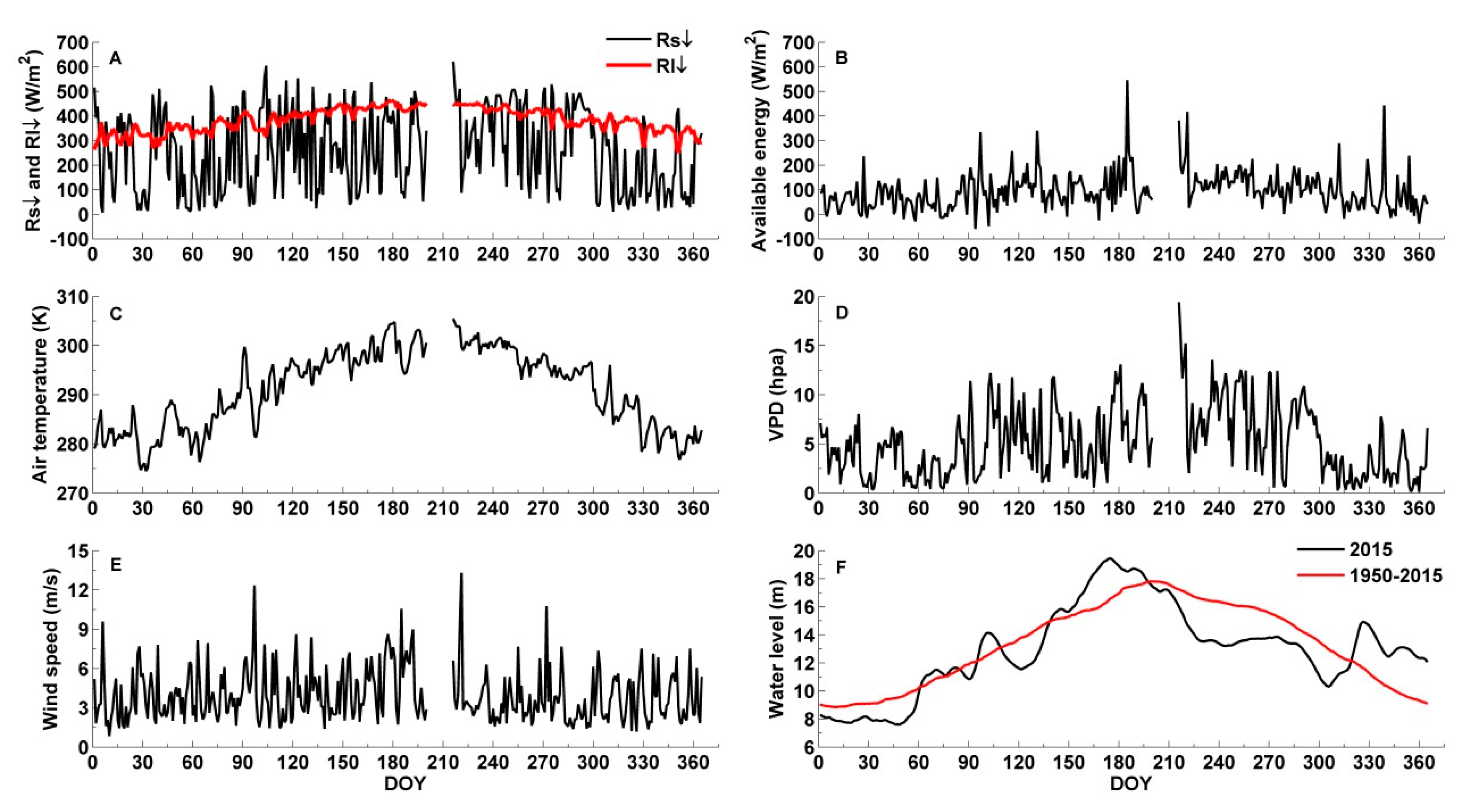
The environmental conditions and energy fluxes (H and LE) of the study site are first described in this section before further analysis. The water level of Poyang Lake usually experiences substantial changes (~8–20 m) throughout the year. The multiyear (1950–2015) daily values of the water level range from 8.8 m to 17.8 m at the Xingzi station. In 2015, the water level fluctuated from 7.6 to 19.5 m, with the minimum and maximum values occurring in DOY 48 and DOY 175, later and earlier than those of the long-term averages, respectively (Figure 3). The high-water (>14 m) period (105 days) in 2015 included DOY (day of the year) times of 100–104, 136–225, and 324–333, whereas the low-water (<12 m) period (130 days) included DOY times of 1–94, 116–128, and 296–318.
On average, Rs↓, Rl↓, A, Ta, VPD, and u were 282.1 W·m−2, 420.5 W·m−2, 111.3 W·m−2, 297.0 K, 6.1 hPa, and 4.6 m/s, respectively, in the high-water period, which were larger than those in the low-water period (i.e., 235.4 W·m−2, 351.2 W·m−2, 73.7 W·m−2, 285.7 K, 3.7 hPa, and 3.8 m/s, respectively). Unimodal seasonal patterns (Figure 3) were observed for the available energy and most of the meteorological variables (i.e., Rs↓, Rl↓, Ta, and VPD). Although the wind speed was also larger for the high-water period than for the low-water period (4.6 m/s vs. 3.8 m/s), compared to Ta, the wind speed exhibited a reduced trend and larger variations throughout the year.
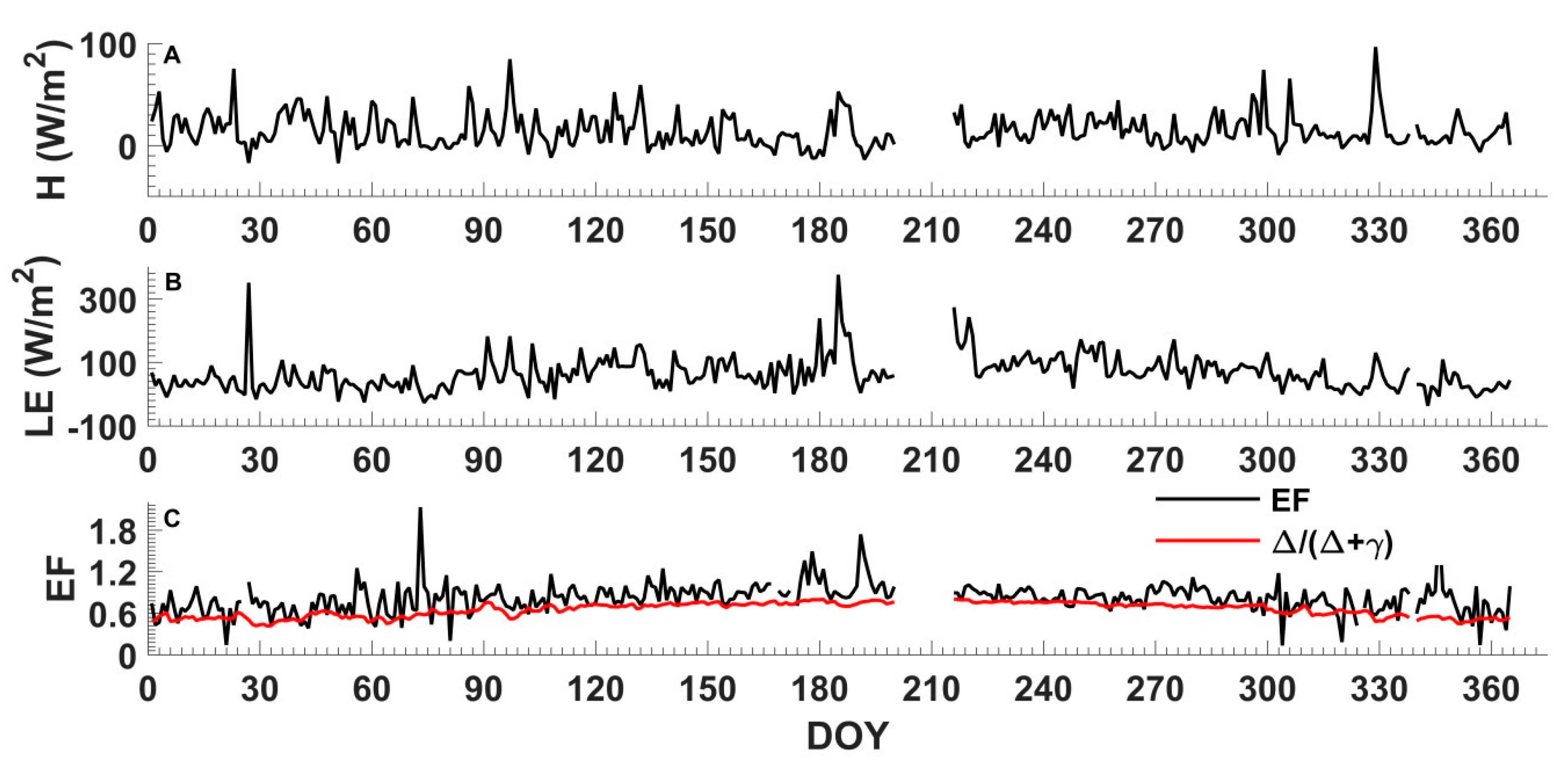
Over-lake observations of energy fluxes in 2015 are shown in Figure 4. LE displayed a unimodal seasonal pattern, which generally matches those of the driving forces (e.g., Rs↓, Rl↓, and Ta). LE peaked in the summer (376.1 W·m−2), and the minimum value (−26.9 W·m−2) occurred in the winter. Compared to LE, H displayed an opposite trend with a smaller mean (11.3 W·m−2) in the high-water period than that in the low-water period (16.9 W·m−2), although the available energy was larger when the water level was higher (92.2 W·m−2 vs. 62.7 W·m−2 on average) (Table 1). One reason for the smaller H in the summer is that a larger portion of the available energy was consumed by LE (EFmean = 0.86, EF = LE/(H + LE)) in the high-water period than that (EFmean = 0.71) in the low-water period.
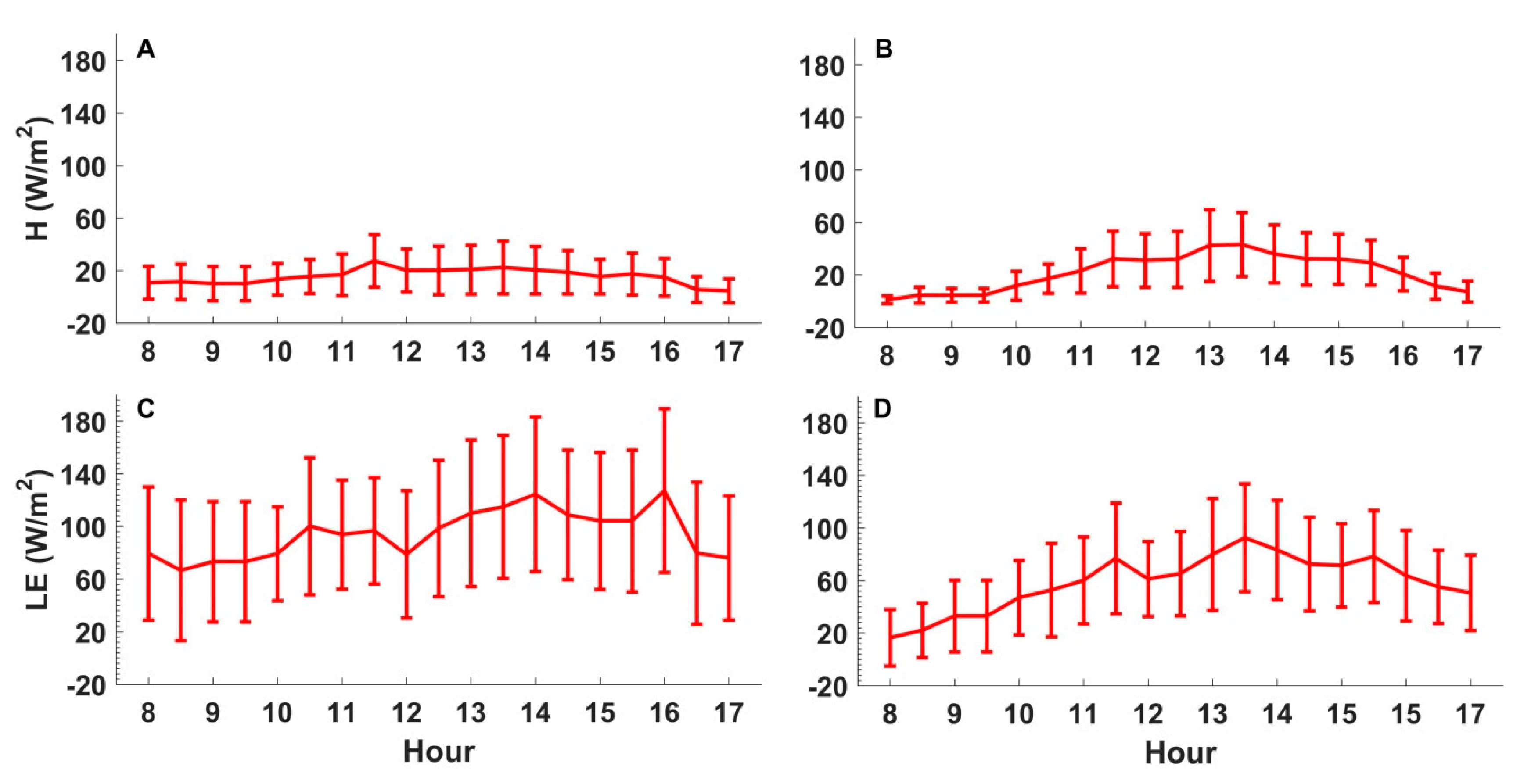
Compared to those in the daily scale scenario, both energy fluxes and the evaporative fraction EF exhibited much larger variations at subdaily scales (Figure 5). However, the diurnal cycle patterns for each variable can also be seen from the averages of the values at the same timings of each day (Figure 5). During the daytime, H exhibited a weak increase over time from early morning and reached its maximum at noon (around 11:30) and then decreased slowly afterward during the high-water period (Figure 5A). Similar, but more obvious, trends for H and LE were found in the low-water period, whose peaks occurred just after noon (i.e., at 13:30) (Figure 5B). In contrast, the LE in the high-water period increased after 9:30, maintained relatively high values from 13:00 until 16:00, and then decreased. These results indicate that, compared to the mudflat, the existence of the water surface smooths the variations in H, delays the time of the peak value of LE, and prolongs the duration of the high values.
4.2. Seasonal and Diurnal Variations in α
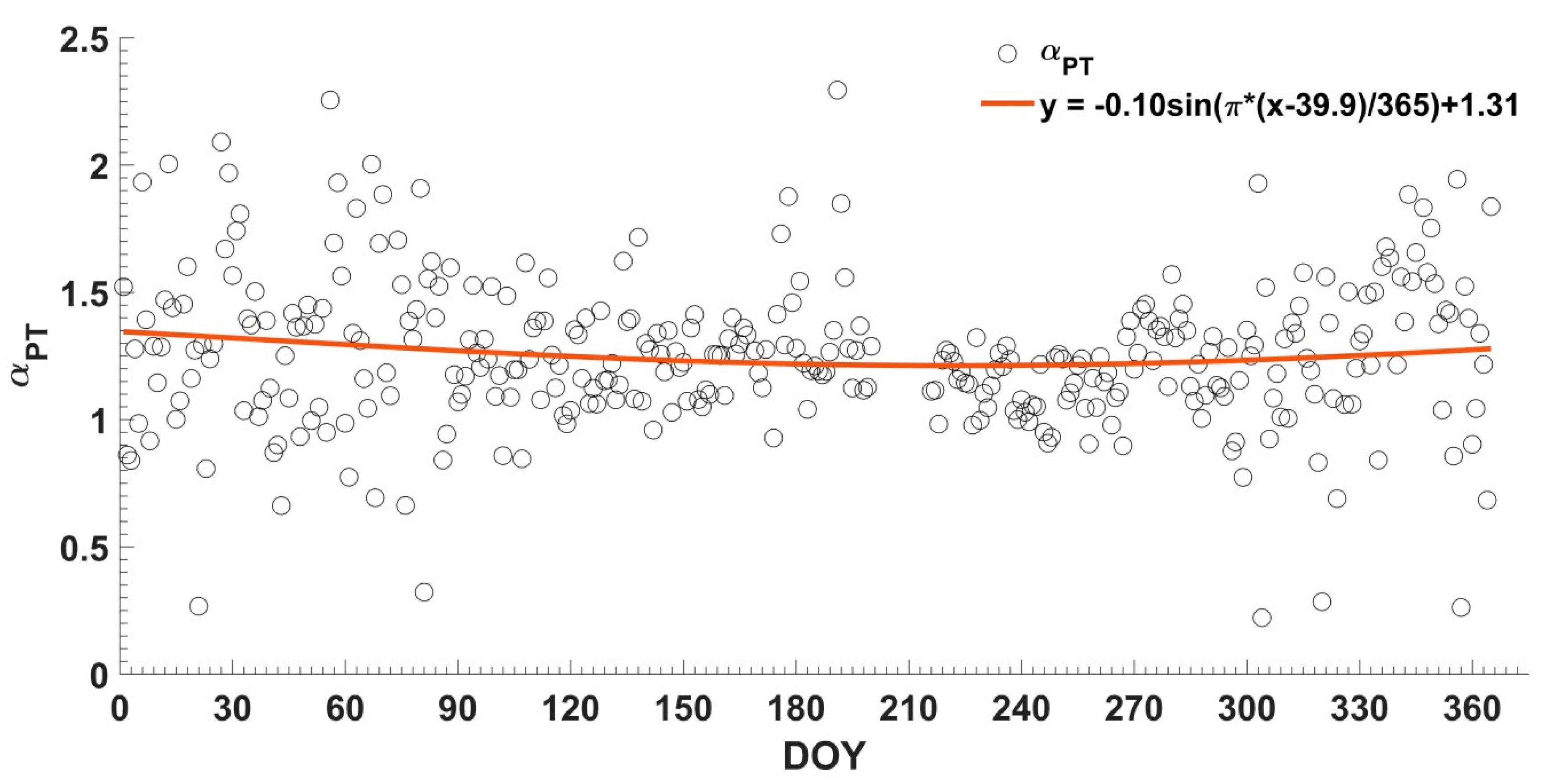
The seasonal and diurnal variations in α are explored in this section. α showed no obvious seasonal trend as Poyang Lake experienced water-rising and water-falling (Figure 6). The mean α was 1.25 during the high-water period, which is close to the widely accepted value of 1.26. A similar but slightly larger mean α (1.29) was found during the low-water period (Figure 6 and Table 2). This result indicates that the PT equation with α = 1.26 can yield reasonable ET estimates on average over the lake and wetland surfaces in Poyang Lake. However, α exhibits large variations around 1.26 during both periods. The standard deviation (sd) in α during the high-water period was 0.19, which is 15.2% of the mean value. In contrast, α during the low-water period exhibited a larger variation (sd = 0.31) than that during the high-water period.
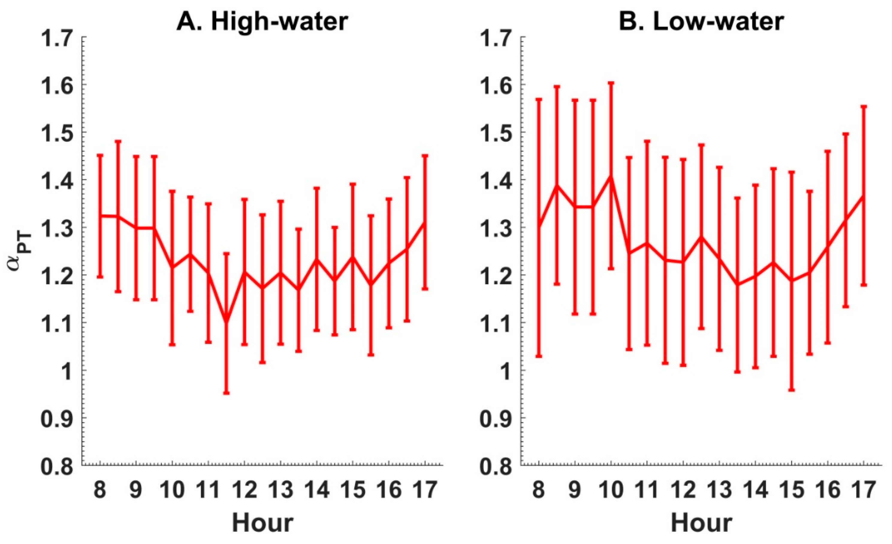
At subdaily scales, α was 1.27 and 1.30 on average during the high-water and low-water periods, respectively, indicating that α = 1.26 is also reasonable at subdaily scales. However, unlike seasonal variations, α generally showed U-shaped diurnal variations during both periods, especially during the high-water period. During the high-water period, α generally decreased from 8:30 to its minimum value at around 11:30, and then increased to relatively high values in the evening (17:00) (Figure 7). The parameter α exhibited large variations during the daytime for the low-water period.
4.3. The Controlling Factors of Parameter α
We performed a stepwise regression analysis to determine the first-order controlling factors of α. We selected the factors that are related to the advection (VPD and u) and the factor that represents the energy supply for sensible and latent heat fluxes (i.e., the available energy) for analysis. Statistics of the regression results are shown in Table 3. RMSE (root mean square error) of the daily predictions were 0.146 and 0.256 during the high-water and low-water periods, respectively, which were relatively small (~11.6%–20.3%) compared to the mean value of α. In addition, although the RMSE of the subdaily predictions (0.214 and 0.329) were larger than those in the daily cases, they were still smaller than 30% of the mean value of α, indicating the capability of the regression equations in explaining the variations α.
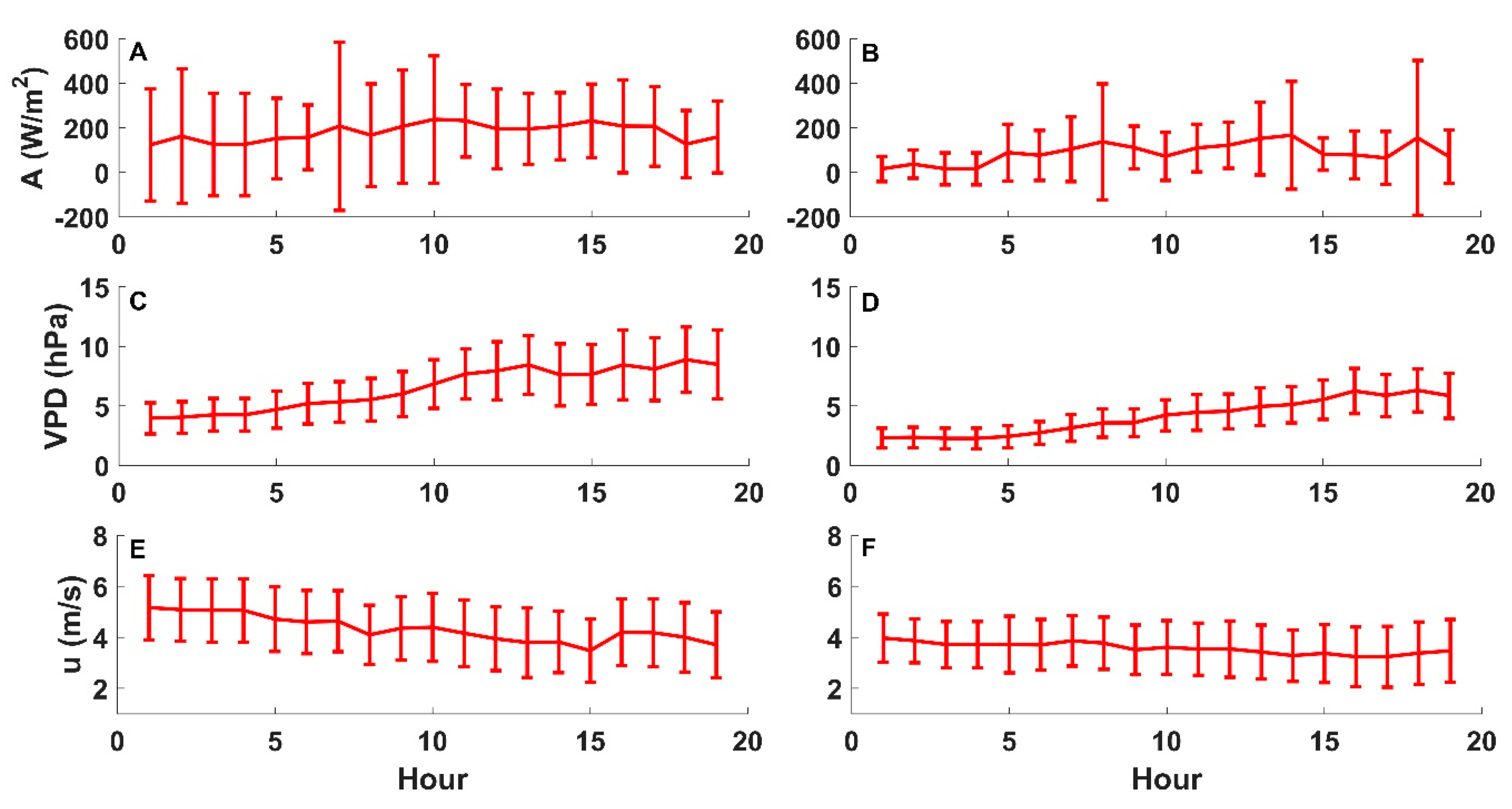
We found that the available energy is negatively correlated with α during both the high-water and low-water periods at subdaily scales (Table 3). Note that the available energy exhibits unimodal patterns at subdaily scales (Figure 8). These results partly explain the U-shaped diurnal patterns in α. VPD exerts positive and negative impacts on subdaily α during the high-water and low-water periods, respectively. In contrast, u exerts positive impacts during both periods. Note that the VPD and wind speed exhibit increasing and decreasing trends, respectively, from 8:00 to 17:00 during both periods (Figure 8). VPD and u tend to cancel out one another’s impacts on α during the high-water period, but amplify one another’s impacts on α during the low-water period.
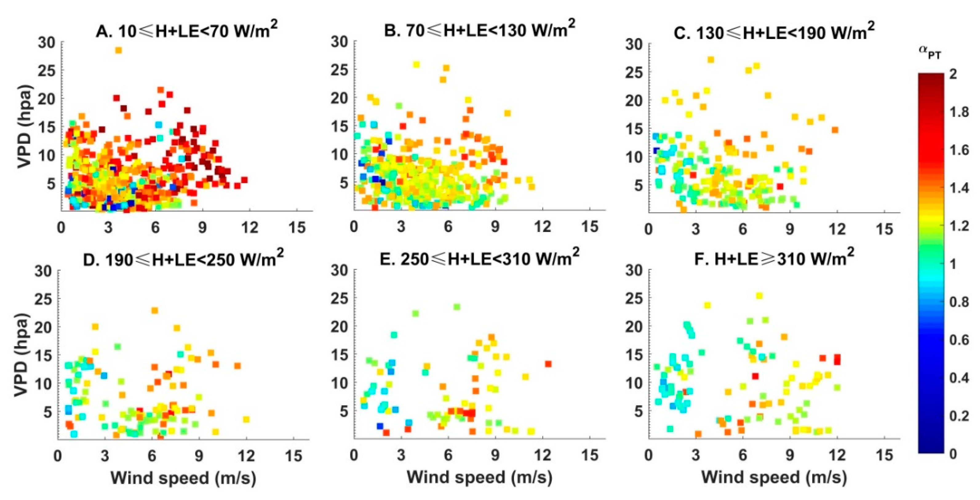
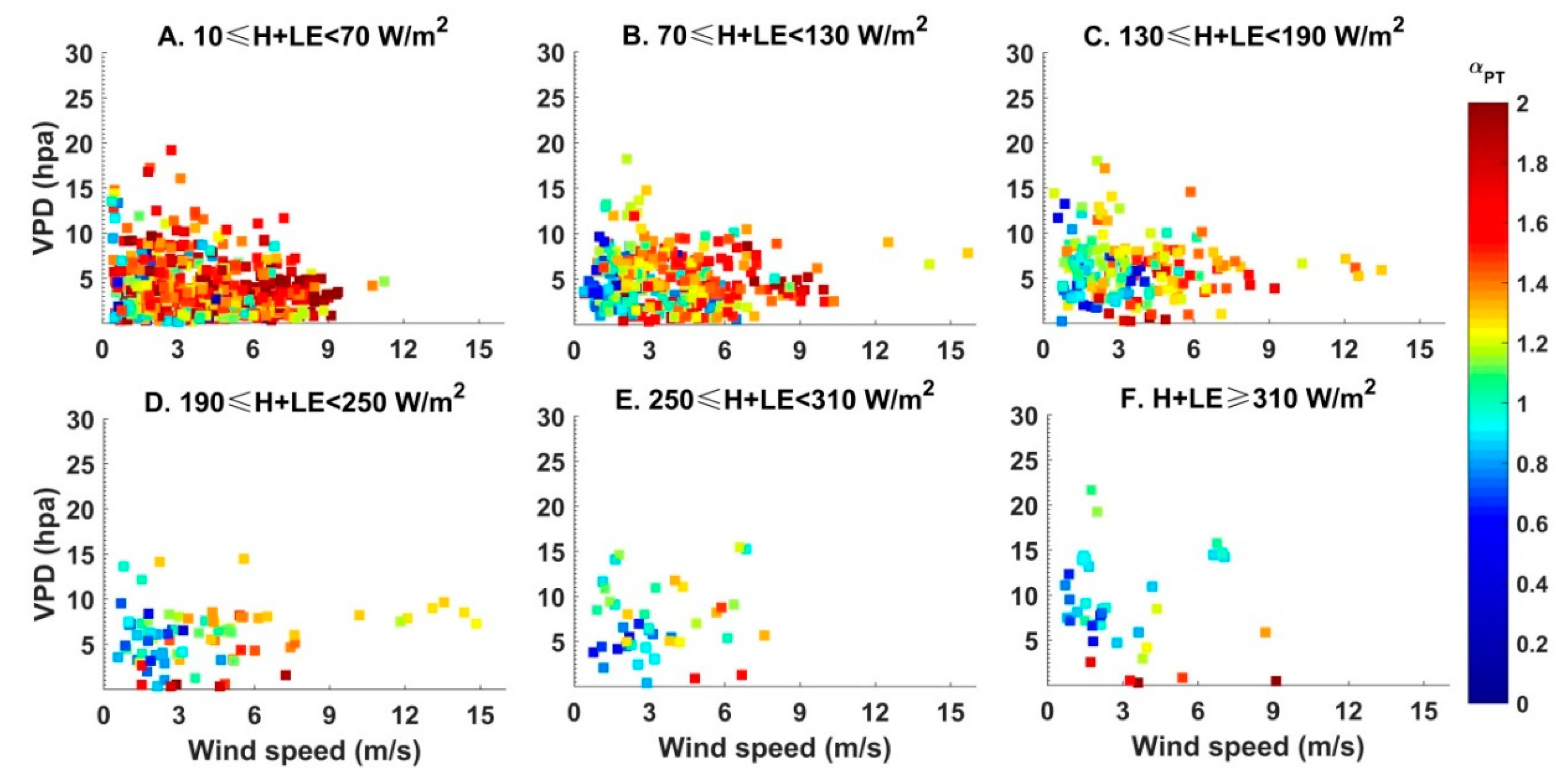
The distributions of α with VPD and u are further analyzed under different available energy ranges (Figure 9 and Figure 10). We found that extreme (large) values generally occur at the lowest available energy range (Figure 9A and Figure 10A). The role of wind speed is significant in most of the available energy ranges at both time scales. Compared to wind speed, VPD exerts less obvious impacts on α. However, α tends to be highest when VPD is close to 0 in most of the available energy ranges. As the available energy increases, α seems to be clustered in different (u, VPD) regions, which can be separated by lines of VPD = a × u + b (Figure 9E,F). For example, the points above and below the line y = x (where x = u and y = VPD) were generally smaller and larger than 1.26, respectively, when the available energy was larger than 310 W·m−2 during the high-water period (e.g., Figure 9E).
5. Discussion
5.1. Contributions of Local Advection and Energy Control to the α Variations
According to Penman’s equation [34], α increases with an increase of wind speed or VPD due to the increase of Ea if the available energy remains constant under water-surface conditions. We estimated the contributions of VPD and u to the α variations by multiplying the standard deviations in VPD and u with their respective coefficients of VPD and u from Table 3. The results are shown in Table 4. Compared to wind speed, VPD exerted much smaller effects on α during the high-water period (i.e., 0.06 vs. 0.11 at a daily scale) (Table 4). This result may be because evaporation from the lake exerted feedbacks on the ambient air humidity. Therefore, a low VPD (small atmospheric demand) does not necessarily indicate that the evaporation is small. Instead, a small VPD may be the result of a large latent heat flux from the lake.
Compared to the high-water period, VPD was found to exert a larger and more negative impact on daily α during the low-water period, indicating that LE decreases with Ea if the air temperature and available energy remain constant. As Granger and Gray [42] noted, VPD reflects the moisture conditions of an unsaturated surface to some extent (i.e., a higher VPD indicates a drier surface). Therefore, this complementary effect may be responsible for the negative correlation between α and VPD during the low-water period.
Our results show that α exhibited no obvious seasonal trend throughout the year, whereas diurnal variation was characterized as U-shaped under wetland surface conditions. This result is consistent with the diurnal U-shaped EF patterns found for vegetative surfaces [43,44]. The stepwise regression analysis shows that a negative correlation exists between the available energy and α, which is partly responsible for the U-shaped diurnal variations over both periods.
Worth noting, compared to daily scales, clusters of subdaily α in different (u, VPD) regions were found across a range of available energy values (Figure 9). The natural speculation is that the two clusters of points that were above and below the y = ax + b line occurred at distant timings. However, this speculation is not true because the DOYs above and below the y = ax + b line exhibited no obvious contrast at each available energy range. A more probable explanation is that the contrasting clusters of points in Figure 9 occurred at the timings in adjacent DOYs or in the same DOY and that the diurnal variations in α caused the emergence of the clusters. For example, the available energy was similar at 8:00, 11:00, and 11:30 in DOY 155 (i.e., 209.7, 206.8, and 194.2 W·m−2, respectively). The corresponding α at those timings was 1.32, 1.09, and 1.07, respectively. In the morning, u was relatively large and VPD was relatively small; thus, the point at 8:00 is located below the y = ax + b line. Further, u decreases and VPD increases with time (Figure 8). Therefore, points at 11:00 and 11:30 are located above the y = ax + b line, and α remained relatively low (1.09 and 1.07) at noon. In summary, because u decreases and VPD increases with time during the day (Figure 8), the points in Figure 9 and Figure 10 tend to rotate in a counterclockwise direction in the u–VPD plane. Because wind speed makes the most (positive) contribution to diurnal α variations (Table 4), clusters of subdaily α in different (u, VPD) regions were found.
5.2. Use of the PT Equation in Changing Surface Conditions
The Priestley–Taylor equation [18] has been widely used as a stand-alone model [45] or as a core part in many ET models [46,47,48,49,50]. The remarkable changes in the water level of Poyang Lake provide a unique opportunity for comparatively studying the variations in α and their controlling factors over water-covered and non-water-covered surfaces. Although the meteorological conditions were quite different between the high-water and low-water periods at our study site, we can still deduce that the existence of the water surface exerted a significant impact on the evaporative process. For example, although the available energy was higher in the high-water period, the H in the high-water period was smaller on average than in the low-water period. In addition, the existence of the water surface remarkably smoothed the variation in LE.
Compared with energy fluxes, no obvious seasonal trend was observed for α. In addition, α = 1.26 is overall feasible for both water-covered and wetland-covered periods. Such results indicate that the PT equation is applicable for LE estimation in our study area if the available energy can be determined. The accuracy of the LE estimation using the PT equation (with α as 1.26) is shown in Table 5. During both the water-covered and wetland-covered periods, the mean biases were less than 5 W·m−2, indicating that the PT equation is feasible in estimating the overall latent heat flux of Poyang Lake at an annual scale. In addition, the root mean square error (RMSE) of the LE predictions at a daily scale was much smaller than the mean measurements in LE, indicating that the PT equation (with α as 1.26) is capable of modeling seasonal ET variations. Worth noting, the RMSE of the LE predictions at a 30 min scale was still less than 50% of the mean ET measurements during the water-covered period. Considerations of the diurnal courses of α and the impacts of wind speed are needed to better model LE at a 30 min scale, especially during the wetland-covered period.
6. Conclusions
The Priestley–Taylor equation has been proven to be robust in estimating the long-term ET of water bodies. However, its sole parameter α may deviate from the widely accepted value of 1.26, especially under ephemeral lake conditions. In this study, we provided a detailed examination of the seasonal and diurnal variability of α over a large ephemeral lake. The results showed that α = 1.26 is overall feasible for not only the water-covered but also the wetland-covered periods. α exhibits no obvious seasonal trend, whereas U-shaped diurnal patterns were found during both periods. Previous studies showed that local advection causes a deviation in α. However, stepwise regression analysis indicates that such U-shaped variations are also correlated with variations in the available energy. Our study indicates that the PT equation is still applicable at subdaily scales if the diurnal variations of α are properly accounted for.
Author Contributions
Conceptualization, G.G. and Y.L.; data curation, X.Z., M.L., and S.W.; formal analysis, G.G.; methodology, G.G. and X.Z.; resources, M.L. and S.W.; writing—original draft, G.G.; writing—review and editing, Y.L. and X.P. All authors have read and agreed to the published version of the manuscript.
Funding
Our research is jointly funded by the National Natural Science Foundation of China (41601033), the State Key Program of National Natural Science of China (41430855), the Talent Introduction Project of the Nanjing Institute of Geography and Limnology, Chinese Academy of Sciences (NIGLAS2018GH06), and the Key Project of Water Resources Department of Jiangxi Province, China (KT201506).
Acknowledgments
We thank the two anonymous reviewers for their valuable comments. We thank Guiping Wu for providing the figure of the study area in this paper. The water level data of Xingzi station were acquired from the Hydrological Bureau of Jiangxi Province (http://www.jxssw.gov.cn/).
Conflicts of Interest
The authors declare no conflict of interest.
References
- Downing, J.A.; Prairie, Y.T.; Cole, J.J.; Duarte, C.M.; Tranvik, L.J.; Striegl, R.G.; McDowell, W.H.; Kortelainen, P.; Caraco, N.F.; Melack, J.M.; et al. The global abundance and size distribution of lakes, ponds, and impoundments. Limnol. Oceanogr. 2006, 51, 2388–2397. [Google Scholar] [CrossRef] [Green Version]
- Polsenaere, P.; Deborde, J.; Detandt, G.; Vidal, L.O.; Perez, M.A.P.; Marieu, V.; Abril, G. Thermal enhancement of gas transfer velocity of CO2 in an Amazon floodplain lake revealed by eddy covariance measurements. Geophys. Res. Lett. 2013, 40, 1734–1740. [Google Scholar] [CrossRef] [Green Version]
- Long, Z.; Perrie, W.; Gyakum, J.; Caya, D.; Laprise, R. Northern lake impacts on local seasonal climate. J. Hydrometeorol. 2007, 8, 881–896. [Google Scholar] [CrossRef] [Green Version]
- Sharma, A.; Hamlet, A.F.; Fernando, H.J.S.; Catlett, C.E.; Horton, D.E.; Kotamarthi, V.R.; Kristovich, D.A.R.; Packman, A.I.; Tank, J.L.; Wuebbles, D.J. The Need for an Integrated Land-Lake-Atmosphere Modeling System, Exemplified by North America’s Great Lakes Region. Earths Future 2018, 6, 1366–1379. [Google Scholar] [CrossRef]
- Rouse, W.R.; Oswald, C.J.; Binyamin, J.; Spence, C.R.; Schertzer, W.M.; Blanken, P.D.; Bussieres, N.; Duguay, C.R. The role of northern lakes in a regional energy balance. J. Hydrometeorol. 2005, 6, 291–305. [Google Scholar] [CrossRef]
- Beyrich, F.; Leps, J.P.; Mauder, M.; Bange, J.; Foken, T.; Huneke, S.; Lohse, H.; Ludi, A.; Meijninger, W.M.L.; Mironov, D.; et al. Area-averaged surface fluxes over the litfass region based on eddy-covariance measurements. Bound. Layer Meteorol. 2006, 121, 33–65. [Google Scholar] [CrossRef]
- Xue, P.F.; Pal, J.S.; Ye, X.Y.; Lenters, J.D.; Huang, C.F.; Chu, P.Y. Improving the Simulation of Large Lakes in Regional Climate Modeling: Two-Way Lake-Atmosphere Coupling with a 3D Hydrodynamic Model of the Great Lakes. J. Climate 2017, 30, 1605–1627. [Google Scholar] [CrossRef]
- Dutra, E.; Stepanenko, V.M.; Balsamo, G.; Viterbo, P.; Miranda, P.M.A.; Mironov, D.; Schar, C. An offline study of the impact of lakes on the performance of the ECMWF surface scheme. Boreal. Environ. Res. 2010, 15, 100–112. [Google Scholar]
- Gu, H.P.; Jin, J.M.; Wu, Y.H.; Ek, M.B.; Subin, Z.M. Calibration and validation of lake surface temperature simulations with the coupled WRF-lake model. Clim. Chang. 2015, 129, 471–483. [Google Scholar] [CrossRef]
- McDonald, C.P.; Rover, J.A.; Stets, E.G.; Striegl, R.G. The regional abundance and size distribution of lakes and reservoirs in the United States and implications for estimates of global lake extent. Limnol. Oceanogr. 2012, 57, 597–606. [Google Scholar] [CrossRef]
- Liu, Y.B.; Wu, G.P.; Zhao, X.S. Recent declines in China’s largest freshwater lake: Trend or regime shift? Environ. Res. Lett. 2013, 8. [Google Scholar] [CrossRef]
- Liu, Y.B.; Song, P.; Peng, J.; Fu, Q.N.; Dou, C.C. Recent increased frequency of drought events in Poyang Lake Basin, China: Climate change or anthropogenic effects? Hydro-Climatol. Var. Chang. 2011, 344, 99–104. [Google Scholar]
- Granger, R.J.; Hedstrom, N. Modelling hourly rates of evaporation from small lakes. Hydrol. Earth Syst. Sci. 2011, 15, 267–277. [Google Scholar] [CrossRef] [Green Version]
- Lenters, J.D.; Kratz, T.K.; Bowser, C.J. Effects of climate variability on lake evaporation: Results from a long-term energy budget study of Sparkling Lake, northern Wisconsin (USA). J. Hydrol. 2005, 308, 168–195. [Google Scholar] [CrossRef]
- Bouin, M.N.; Caniaux, G.; Traulle, O.; Legain, D.; Le Moigne, P. Long-term heat exchanges over a Mediterranean lagoon. J. Geophys. Res. Atmos. 2012, 117. [Google Scholar] [CrossRef]
- Nordbo, A.; Launiainen, S.; Mammarella, I.; Lepparanta, M.; Huotari, J.; Ojala, A.; Vesala, T. Long-term energy flux measurements and energy balance over a small boreal lake using eddy covariance technique. J. Geophys. Res. Atmos. 2011, 116. [Google Scholar] [CrossRef]
- Assouline, S.; Tyler, S.W.; Tanny, J.; Cohen, S.; Bou-Zeid, E.; Parlange, M.B.; Katul, G.G. Evaporation from three water bodies of different sizes and climates: Measurements and scaling analysis. Adv. Water Resour. 2008, 31, 160–172. [Google Scholar] [CrossRef]
- Priestley, C.H.B.; Taylor, R.J. Assessment of Surface Heat-Flux and Evaporation Using Large-Scale Parameters. Mon. Weather Rev. 1972, 100, 81. [Google Scholar] [CrossRef]
- Debruin, H.A.R. A Model for the Priestley-Taylor Parameter-Alpha. J. Clim. Appl. Meteorol. 1983, 22, 572–578. [Google Scholar] [CrossRef] [Green Version]
- Eichinger, W.E.; Parlange, M.B.; Stricker, H. On the concept of equilibrium evaporation and the value of the Priestley-Taylor coefficient. Water Resour. Res. 1996, 32, 161–164. [Google Scholar] [CrossRef] [Green Version]
- Keskin, M.E.; Terzi, O. Evaporation estimation models for Lake Egirdir, Turkey. Hydrol. Process. 2006, 20, 2381–2391. [Google Scholar] [CrossRef]
- Delclaux, F.; Coudrain, A.; Condom, T. Evaporation estimation on Lake Titicaca: A synthesis review and modelling. Hydrol. Process. 2007, 21, 1664–1677. [Google Scholar] [CrossRef]
- Guo, X.F.; Liu, H.P.; Yang, K. On the Application of the Priestley-Taylor Relation on Sub-daily Time Scales. Bound. Layer Meteorol. 2015, 156, 489–499. [Google Scholar] [CrossRef]
- Assouline, S.; Li, D.; Tyler, S.; Tanny, J.; Cohen, S.; Bou-Zeid, E.; Parlange, M.; Katul, G.G. On the variability of the Priestley-Taylor coefficient over water bodies. Water Resour. Res. 2016, 52, 150–163. [Google Scholar] [CrossRef] [Green Version]
- Soucha, C.; Wolfe, C.P.; Grimmtind, C.S.B. Wetland evaporation and energy partitioning: Indiana Dunes National Lakeshore. J. Hydrol. 1996, 184, 189–208. [Google Scholar] [CrossRef]
- Drexler, J.Z.; Snyder, R.L.; Spano, D.; Paw, K.T.U. A review of models and micrometeorological methods used to estimate wetland evapotranspiration. Hydrol. Process 2004, 18, 2071–2101. [Google Scholar] [CrossRef]
- Zhao, X.S.; Liu, Y.B. Phase transition of surface energy exchange in China’s largest freshwater lake. Agr. For. Meteorol. 2017, 244, 98–110. [Google Scholar] [CrossRef]
- Zhao, X.S.; Liu, Y.B. Variability of Surface Heat Fluxes and Its Driving Forces at Different Time Scales Over a Large Ephemeral Lake in China. J. Geophys. Res. Atmos. 2018, 123, 4939–4957. [Google Scholar] [CrossRef]
- Bowen, I.S. The ratio of heat losses by conduction and by evaporation from any water surface. Phys. Rev. 1926, 27, 779–787. [Google Scholar] [CrossRef] [Green Version]
- Raupach, M.R. Combination theory and equilibrium evaporation. Q. J. Roy Meteorol. Soc. 2001, 127, 1149–1181. [Google Scholar] [CrossRef]
- Blanken, P.D.; Spence, C.; Hedstrorn, N.; Lenters, J.D. Evaporation from Lake Superior: 1. Physical controls and processes. J. Great Lakes Res. 2011, 37, 707–716. [Google Scholar] [CrossRef]
- Spence, C.; Blanken, P.D.; Hedstrom, N.; Fortin, V.; Wilson, H. Evaporation from Lake Superior: 2 Spatial distribution and variability. J. Great Lakes Res. 2011, 37, 717–724. [Google Scholar] [CrossRef]
- Spence, C.; Blanken, P.D.; Lenters, J.D.; Hedstrom, N. The Importance of Spring and Autumn Atmospheric Conditions for the Evaporation Regime of Lake Superior. J. Hydrometeorol. 2013, 14, 1647–1658. [Google Scholar] [CrossRef]
- Penman, H.L. Natural Evaporation from Open Water, Bare Soil and Grass. Proc. R. Soc. Lon. Ser. A 1948, 193, 120–145. [Google Scholar] [CrossRef] [Green Version]
- Wu, G.P.; Liu, Y.B. Capturing variations in inundation with satellite remote sensing in a morphologically complex, large lake. J. Hydrol. 2015, 523, 14–23. [Google Scholar] [CrossRef]
- Wu, G.P.; Liu, Y.B. Combining Multispectral Imagery with in situ Topographic Data Reveals Complex Water Level Variation in China’s Largest Freshwater Lake. Remote Sens. 2015, 7, 13466–13484. [Google Scholar] [CrossRef] [Green Version]
- Liu, Y.; Wu, G. Hydroclimatological influences on recently increased droughts in China’s largest freshwater lake. Hydrol. Earth Syst. Sci. 2016, 20, 93–107. [Google Scholar] [CrossRef] [Green Version]
- Li, P.; Feng, Z.M.; Jiang, L.G.; Liu, Y.; Hu, J.W.; Zhu, J.P. Natural Water Surface of Poyang Lake Monitoring Based on Remote Sensing and the Relationship with Water Level. J. Nat. Resour. 2013, 28, 1556–1568. [Google Scholar]
- Kljun, N.; Calanca, P.; Rotach, M.W.; Schmid, H.P. A simple two-dimensional parameterisation for Flux Footprint Prediction (FFP). Geosci. Model. Dev. 2015, 8, 3695–3713. [Google Scholar] [CrossRef] [Green Version]
- Kljun, N.; Calanca, P.; Rotach, M.W.; Schmid, H.P. A simple parameterisation for flux footprint predictions. Bound. Layer Meteorol. 2004, 112, 503–523. [Google Scholar] [CrossRef]
- Papale, D.; Reichstein, M.; Aubinet, M.; Canfora, E.; Bernhofer, C.; Kutsch, W.; Longdoz, B.; Rambal, S.; Valentini, R.; Vesala, T.; et al. Towards a standardized processing of Net Ecosystem Exchange measured with eddy covariance technique: Algorithms and uncertainty estimation. Biogeosciences 2006, 3, 571–583. [Google Scholar] [CrossRef] [Green Version]
- Granger, R.J.; Gray, D.M. Evaporation from Natural Nonsaturated Surfaces. J. Hydrol. 1989, 111, 21–29. [Google Scholar] [CrossRef]
- Gentine, P.; Entekhabi, D.; Chehbouni, A.; Boulet, G.; Duchemin, B. Analysis of evaporative fraction diurnal behaviour. Agr. For. Meteorol. 2007, 143, 13–29. [Google Scholar] [CrossRef] [Green Version]
- Lhomme, J.P.; Elguero, E. Examination of evaporative fraction diurnal behaviour using a soil-vegetation model coupled with a mixed-layer model. Hydrol. Earth Syst. Sci. 1999, 3, 259–270. [Google Scholar] [CrossRef]
- Fisher, J.B.; Tu, K.P.; Baldocchi, D.D. Global estimates of the land-atmosphere water flux based on monthly AVHRR and ISLSCP-II data, validated at 16 FLUXNET sites. Remote Sens. Environ. 2008, 112, 901–919. [Google Scholar] [CrossRef]
- Garcia, M.; Sandholt, I.; Ceccato, P.; Ridler, M.; Mougin, E.; Kergoat, L.; Morillas, L.; Timouk, F.; Fensholt, R.; Domingo, F. Actual evapotranspiration in drylands derived from in-situ and satellite data: Assessing biophysical constraints. Remote Sens. Environ. 2013, 131, 103–118. [Google Scholar] [CrossRef]
- Liu, Y.B.; Hiyama, T.; Yasunari, T.; Tanaka, H. A nonparametric approach to estimating terrestrial evaporation: Validation in eddy covariance sites. Agr. For. Meteorol. 2012, 157, 49–59. [Google Scholar] [CrossRef]
- Gao, Y.C.; Gan, G.J.; Liu, M.F.; Wang, J.F. Evaluating soil evaporation parameterizations at near-instantaneous scales using surface dryness indices. J. Hydrol. 2016, 541, 1199–1211. [Google Scholar] [CrossRef]
- Gan, G.J.; Gao, Y.C. Estimating time series of land surface energy fluxes using optimized two source energy balance schemes: Model formulation, calibration, and validation. Agr. For. Meteorol. 2015, 208, 62–75. [Google Scholar] [CrossRef]
- Gan, G.; Kang, T.; Yang, S.; Bu, J.; Feng, Z.; Gao, Y. An optimized two source energy balance model based on complementary concept and canopy conductance. Remote Sens. Environ. 2019, 223, 243–256. [Google Scholar] [CrossRef]
Figure 1.
The extent of Poyang Lake and the measuring site in Sheshan Island. The middle panel shows the Landsat 8 images (composites using bands 5, 4, and 3 of the Operational Land Imager, which emphasize the distribution of the water body and vegetation) acquired on 24 August (high-water) and 13 February (low-water). The lower panel shows pictures of the measuring site during the high-water and low-water periods.

Figure 2.
Footprint analysis for the eddy covariance measurement. (A) Cumulative footprint from the wind direction; (B) distribution of the wind direction; (C) source area under stable conditions, where the median values of wind speed were used in the calculation; (D) the source area under unstable conditions, where the median values of wind speed were used in the calculation.

Figure 3.
A–E are seasonal variations in meteorological variables, including the incoming shortwave and longwave radiation (A), the available energy (B), air temperature (C), VPD (D), and wind speed (E). Water level variations at Xingzi station are shown in (F), where black and red lines represent the daily values in 2015 and the averaged daily values during the period of 1950–2015, respectively.

Figure 4.
Seasonal variations in H, LE, and EF in 2015. The outliers of EF when H + LE was close to 0 are not shown in the figure.
Figure 4.
Seasonal variations in H, LE, and EF in 2015. The outliers of EF when H + LE was close to 0 are not shown in the figure.

Figure 5.
Diurnal variations in H and LE in 2015. (A) and (C) indicate the high-water period, and (B) and (D) indicate the low-water period. The length of the bar in each subfigure represents the value of the standard deviation of the energy fluxes.
Figure 5.
Diurnal variations in H and LE in 2015. (A) and (C) indicate the high-water period, and (B) and (D) indicate the low-water period. The length of the bar in each subfigure represents the value of the standard deviation of the energy fluxes.

Figure 6.
Seasonal variations in α in 2015.

Figure 7.
Diurnal variations in α during the high-water (A) and low-water (B) periods in 2015. The length of the bar in each subfigure represents the value of the standard deviation of the variable.
Figure 7.
Diurnal variations in α during the high-water (A) and low-water (B) periods in 2015. The length of the bar in each subfigure represents the value of the standard deviation of the variable.

Figure 8.
Diurnal variations in A, VPD, and u during the high-water (A, C, E) and low-water (B, D, F) periods in 2015. The length of the bar in each subfigure represents the value of the standard deviation of the variable.
Figure 8.
Diurnal variations in A, VPD, and u during the high-water (A, C, E) and low-water (B, D, F) periods in 2015. The length of the bar in each subfigure represents the value of the standard deviation of the variable.

Figure 9.
Distributions of 30 min scale α with respect to VPD and wind speed under a range of available energy conditions during high-water period.
Figure 9.
Distributions of 30 min scale α with respect to VPD and wind speed under a range of available energy conditions during high-water period.

Figure 10.
Distributions of 30 min scale α with respect to VPD and wind speed under a range of available energy conditions during the low-water period.
Figure 10.
Distributions of 30 min scale α with respect to VPD and wind speed under a range of available energy conditions during the low-water period.


Table 1.
Statistics of daily H, LE, and EF.
| Variables | The Entire Period | High-Water Period | Low-Water Period | ||||||
|---|---|---|---|---|---|---|---|---|---|
| Min | Max | Mean | Min | Max | Mean | Min | Max | Mean | |
| H (W·m−2) | −17.5 | 96.8 | 16.3 | −13.8 | 96.8 | 11.3 | −17.5 | 75.4 | 16.9 |
| LE (W·m−2) | −26.9 | 376.1 | 68.9 | −12.6 | 376.1 | 80.9 | −26.9 | 351.1 | 45.8 |
| EF (-) | −3.78 | 2.13 | 0.81 | −1.07 | 1.73 | 0.86 | −3.78 | 2.13 | 0.71 |
Table 2.
Statistics of the daily and subdaily α.
| Time scales | The Entire Period | High-Water Period | Low-Water Period | ||||||
|---|---|---|---|---|---|---|---|---|---|
| Min | Max | Mean | Min | Max | Mean | Min | Max | Mean | |
| Daily | 0.22 | 2.29 | 1.27 | 0.69 | 2.29 | 1.25 | 0.22 | 2.26 | 1.29 |
| Subdaily | 0.01 | 2.12 | 1.29 | 0.16 | 2.11 | 1.27 | 0.01 | 2.12 | 1.30 |
Table 3.
Stepwise regression analysis for α during both the high-water and low-water periods at daily and subdaily scales. RMSE represents the root mean squared error of the prediction from the regression equation. r represents the correlation coefficient between the predictions and “ground-truth” α.
| Timescales | Variables | Statistics for Coefficients | Statistics for the Regression Equation | |||
|---|---|---|---|---|---|---|
| Daily | High-water | Coefficients | Status | Pcoeff | RMSE | r |
| A | −0.0016 | In | <0.001 | 0.146 | 0.66 | |
| VPD | 0.0148 | In | 0.001 | |||
| u | 0.0465 | In | <0.001 | |||
| Constant | 1.102 | |||||
| Low-water | Coefficients | Status | Pcoeff | RMSE | R2 | |
| A | −9.503 × 10⁻⁴ | Out | 0.106 | 0.256 | 0.58 | |
| VPD | −0.0340 | In | <0.001 | |||
| u | 0.084 | In | <0.001 | |||
| Constant | 1.096 | |||||
| 30 min | High-water | Coefficients | Status | Pcoeff | RMSE | R2 |
| A | −8.730 × 10⁻⁴ | In | <0.001 | 0.214 | 0.46 | |
| VPD | 0.0098 | In | <0.001 | |||
| u | 0.0317 | In | <0.001 | |||
| Constant | 1.168 | |||||
| Low-water | Coefficients | Status | Pcoeff | RMSE | R2 | |
| A | −0.0015 | In | <0.001 | 0.329 | 0.47 | |
| VPD | −0.0065 | In | 0.02 | |||
| u | 0.0573 | In | <0.001 | |||
| Constant | 1.197 | |||||
Table 4.
Magnitudes of contributions of VPD and u to α variations.
| Variables | Daily | 30 min | ||
|---|---|---|---|---|
| High-Water | Low-Water | High-Water | Low-Water | |
| VPD | 0.06 | −0.08 | 0.05 | −0.02 |
| u | 0.11 | 0.16 | 0.08 | 0.13 |
| A | −0.12 | 0 | −0.09 | −0.12 |
Table 5.
Accuracy of the LE estimation using the PT equation (α = 1.26) during both periods.
| Time Scales | High-Water | Low-Water | ||||
|---|---|---|---|---|---|---|
| RMSE (W·m−2) | Bias (W·m−2) | Mean (W·m−2) | RMSE (W·m−2) | Bias (W·m−2) | Mean (W·m−2) | |
| Daily | 11.2 | 3.4 | 105.9 | 19.1 | 1.5 | 70.4 |
| 30 min | 23.3 | 4.1 | 105.9 | 28.4 | 4.2 | 70.4 |
© 2020 by the authors. Licensee MDPI, Basel, Switzerland. This article is an open access article distributed under the terms and conditions of the Creative Commons Attribution (CC BY) license (http://creativecommons.org/licenses/by/4.0/).
Share and Cite
MDPI and ACS Style
Gan, G.; Liu, Y.; Pan, X.; Zhao, X.; Li, M.; Wang, S. Seasonal and Diurnal Variations in the Priestley–Taylor Coefficient for a Large Ephemeral Lake. Water 2020, 12, 849. https://doi.org/10.3390/w12030849
AMA Style
Gan G, Liu Y, Pan X, Zhao X, Li M, Wang S. Seasonal and Diurnal Variations in the Priestley–Taylor Coefficient for a Large Ephemeral Lake. Water. 2020; 12(3):849. https://doi.org/10.3390/w12030849
Chicago/Turabian StyleGan, Guojing, Yuanbo Liu, Xin Pan, Xiaosong Zhao, Mei Li, and Shigang Wang. 2020. "Seasonal and Diurnal Variations in the Priestley–Taylor Coefficient for a Large Ephemeral Lake" Water 12, no. 3: 849. https://doi.org/10.3390/w12030849
Note that from the first issue of 2016, this journal uses article numbers instead of page numbers. See further details here.