Fractal-Heuristic Method of Water Quality Sensor Locations in Water Supply Network

Abstract

The article presents a new methodology for the selection of the water quality monitoring sensor locations using the water quality model created by means of the EPANET 2.0 software (United States Environmental Protection Agency (USEPA), Durham, NC, USA). The model represents the propagation of free chlorine in a water supply network, in conjunction with the heuristic method, applying the elements of fractal geometry. In the first stage, a subarea is determined, while in the second, a specific node for the location of the measuring point is indicated. The process of determining the location is based on a ranking method, in which the usefulness of individual subareas and measuring nodes is determined by means of a formula taking into account the amount of water intake, the required level of water supply and the effects of a lack of water supply, as well as the calculated concentration of free chlorine. The application of the method requires the construction and calibration of a numerical model of free chlorine decay in the network, as well as the knowledge on the location of the objects of particular importance for the network users. The proposed method will be applied in an existing water supply network of approximately 50,000 recipients.

1. Introduction

The water quality monitoring is the most important measure ensuring the supply of water with high quality, meeting the requirements included in the legal regulations of each country. These regulations usually indicate that monitoring is to be carried out at the points representative of the water quality in the distribution system, in which the sensors detecting the contamination events can be placed. However, the procedure for determining the location of such points is not specified. Sensors cannot be placed at every network node, due to high costs and other constrains. Numerous methods have been developed all over the world to solve the monitor location problem; however, until now there has been no universal method of determining the representative sensor locations.

A large variety of approaches have been proposed to locate sensors with different methodologies and objectives. Hart and Murray [1] reviewed the available literature on the monitoring sensors strategies until 2009, and they suggested several key issues that need to be addressed in the future work. Rathi and Gupta [2,3], and Rahti et al. [4] presented a critical review of single- and multi-objective sensor location problems, considering general parameters for the comparison of different methodologies. In each group of methodologies (single/multi objective), they indicated the main objectives, the methodology used or optimization solver, and the required sensors—fixed or variable.

The first studies on the placement of the water quality monitoring stations using Demand Coverage (DC) method were presented by Lee and Deiniger [5]. The method is based on the principle that a monitoring station covers a node if a sufficient quantity of water under steady state flows from this node to the monitoring station for a given scenario of demand pattern, as well as the water quality decreases with the time and distance from the source. Analogous studies were performed by Kumar et al. [6]. They solved the sensor placement problem by means of mixed integer programming, using a greedy heuristic based algorithm. Al-Zahrani and Moeid [7,8] modified the demand coverage to help in identifying the water quality monitoring stations in a water distribution network using a Genetic Algorithm (GA). They proposed that the water quality monitoring stations location should be based on the quantity of the flow, assuming that the water quality at a downstream node is lower than the water quality at an upstream node. Harmant et al. [9] modified the objective function to introduce time dependence and water quality into the Demand Coverage model. They proposed a covering matrix which defines the link between each network node; the algorithm selects the most representative points in terms of consumption and water deterioration. Tryby and Uber [10] derived the Demand Coverage concept using mixed integer linear programming to solve the problem and the water age as the basis for determining the sample representativeness. Woo et al. [11] applied the method of minimal path enumeration with list processing to construct the coverage matrix and to determine all the flow paths. With the coverage matrix, they used integer programming to solve the problem. Shuming Liu et al. [12] presented the development of a Demand Coverage Index (DCI) method for finding the optimal locations of monitoring stations under multiple demand patterns. Special consideration was given to the method of evaluating the representativeness of a node at an extended period under unsteady hydraulics conditions.

In both single- and multi-objective methodologies, many authors have used heuristic methods mainly to simplify the problem. Kumar et al. [13] and Kansal et al. [14] proposed a coverage matrix and suggested a heuristic method to locate the monitoring stations one by one, by selecting the best location first and modifying the coverage matrix by eliminating the nodes already covered to select next stations. Ghimire and Barkdoll [15,16] presented two heuristic methods of selecting the sensor location. In the first one, the sensors were placed at the junctions characterized by the highest water demand. In the other method, sensors were placed at the junctions with the greatest mass of flowing water (mass-based approach). Rathi and Gupta [2] also suggested a heuristic method for choosing the location of monitoring stations based on the concept of ‘construction of shortest travel time trees’ to achieve the targeted aim. A related approach of using expert information to rank the potential sensor locations was presented by Xu et al. [16]. A user provides the preference values for the properties of a “desirable” sensor location, such as proximity to critical facilities, which are used to rank the desirability of sensor locations. The spatial information, e.g., Geographic Information System (GIS) and/or a utility network model can be integrated to ensure good coverage of the network. A heuristic method based on the elements of fractal geometry theory was put forward by Kowalski et al. [17,18,19]. In this approach, the elements of risk theory were assumed as the basis for evaluating the correctness of the indicated measurement sensor locations. In this methodology, significant risk parameters were distinguished, including: Volume of water in the nonmonitored network, maximum detection time of a pollutant from the moment of its appearance, and detection time relative to the volume of water in the monitored network. Kessler et al. [20] added to the coverage problem an all-pairs shortest path algorithm and the construction of a pollution matrix, containing the data regarding the nodes which are contaminated by many possible contamination events. In their study, the definition of a contaminated node refers to the contaminant concentration which exceeds the allowable value. Ostfeld and Salomons [21] expanded the study of Kessler et al. [20] by introducing a randomized pollution matrix which holds a set of randomly generated multiple injection locations and times. The values in the matrix determine if a node was contaminated at a specific random event. Additionally, Zhao et al. [22] used the randomized pollution matrix concept in their study, where each value of the matrix represents an assessment of the consumption of the contaminated water assuming that the sensor in the related node is the first to detect the event. The sensor placement algorithm was based on greedy heuristic and convex relaxation.

A different concept was presented by Conzollino et al. [23]. They formulated a Lagrangian advection method which estimates the time of each flow path in the network. A stochastic approach was proposed, aiming at the optimal allocation of the increasing sets of monitoring stations for the early detection of the intentional contamination in water distribution networks. The approach is based on the use of the Monte Carlo technique for the generation of a number of time-varying hydraulic scenarios, each consisting of a succession of steady conditions related to different users’ water demands. Berry et al. [24] formulated a low memory Lagrangian relaxation method which simplified the problem by assigning a penalty to the constraint violation. The Lagrangian relaxation method was used in order to compute lower bounds on the expected impact of suites of contamination events. Berry et al. [25] and Hart [26] presented the Teva Spot toolkit which combines general purpose heuristics with integer programming and bounding algorithms. The Sensor Placement Optimization Tool (Teva-Spot) is a free program developed by USEPA. It uses a graphical user interface which can be integrated with the EPANET software in terms of the hydraulic analysis portion of the optimal sensor placement algorithms.

Drinking water utilities around the world are vulnerable to various types of bioterrorist attacks; hence, some studies were dedicated specifically to this topic, e.g., [21,27,28]. Most of the research has focused on deriving the methodologies and algorithms that a presumptive contamination of water would be detected as soon as possible. In recent years, the interest in the methods for determining the location of water quality monitoring stations based on the measurement of free chlorine concentration (chlorine residuals) has also appeared [29]. Chlorine is the most commonly used disinfectant in the world because of its comparatively low price, effectiveness in killing bacteria, and chemical stability in water. In the water distribution network, chlorine can be consumed in the bulk liquid phase, in reaction with ammonia, iron, and organic compounds. Additionally, chlorine disappears due to its interactions with deposits, as well as due to corrosion and biomass growth on the inner pipe walls [30,31]. It is difficult to predict the chlorine decay in large distribution systems; therefore, when testing the chlorine decay, it seems easier to separate the reactions associated with the bulk water from those associated with the pipe wall [32,33,34,35]. The chlorine decay within the water supply network may lead to the degradation of water quality and, thus, poses potential microbial risks to humans. Therefore, it is important to maintain residual chlorine throughout the water supply network within the desirable levels [36,37,38]. It is also important not to exceed the recommended dose of chlorine as this can lead to the formation of disinfection by-products that are harmful to the human health. Researchers are looking for the methods and optimization algorithms to monitor the disinfection by-products (Depla et al. 2018, Brown and Emmert, 2006) [39,40].

Despite the multitude of different methods, none of them enables simultaneous consideration of so many different factors, such as the concentration of free chlorine, reliability of supplying water of adequate quality required by customers, the consequences of failure to meet these requirements, the amount of water demand, and the exclusion of the location of measuring points too close to each other. One of the first methods, which took into account most of the abovementioned factors, was developed by the authors in 2013 [17,18,19]. It was a ranking method in which four criteria of equal weight were used, including water demand, reliability of supplying water of adequate quality required by customers, the consequences of failure to meet these requirements, and water age. The water age was a parameter only providing the information on the possibility of the recontamination of the supplied water. Its estimation may be employed when there is no data on the actual changes in water quality.

The purpose of the article is to present a methodology for the selection of water quality monitoring sensor locations taking into account concentration of free chlorine, reliability of supplying water of adequate quality required by customers, the consequences of failure to meet these requirements, the amount of water demand, and the exclusion of the location of measuring points too close to each other. Similar to the solution developed by the authors from 2013 [17], this is a heuristic, ranking method. The authors proposed the application of the free chlorine concentration instead of the age of water. The assessment of such concentration requires a numerical water quality model, created using the EPANET 2.0 software (USEPA). The application of the fractal geometry elements allowed the exclusion of the location of measuring points too close to each other. The proposed new method was tested for the existing water supply system. The obtained location of the monitoring sensor locations was compared with the locations determined on the basis of two other ranking methods using the age of water and the volume of water demand as the only criteria.

2. Materials and Methods

The method presented in the paper is directed at indicating the location of sensors monitoring the quality of water transported through the distribution network. The water quality measurement was limited to the concentration of free chlorine, treated as an indicator of microbial safety of the supplied water.

In order to determine the sensors location, the authors adopted a ranking method carried out in two stages—ranking of subareas and ranking of junctions in the indicated subareas. The following set of rules has been used as an equal weight ranking criteria:

(1) Free chlorine concentration coefficient c;

(2) Water demand coefficient Q;

(3) Required reliability level of the water delivery a;

(4) Estimated results of failure to supply water with the required quality b.

In order to identify the greatest benefit from monitoring point of view location of water quality sensors, the significance index W, based on the criteria described above, was used:

$$W=Q·a·b·c$$

(1)

The higher value of index W indicates the greater benefit of locating the sensor at a given point. It allows creating a ranking list of all analyzed subareas/junctions.

The sensors are placed only in the network junctions. The first of them is obligatorily located in the pumping station. In the case of equal value of the W index for various subareas or junctions, the higher position in the ranking was given to the one with the higher value of the Q coefficient, which corresponds to a greater number of water recipients or more important public institution or industrial plant.

The values of Q, a, b, and c coefficients are proposed to be dimensionless, according to a five-point scale. Such scale is often employed for estimating the risk connected with the safety of water supply to recipients [41,42,43]. The ranking index W is calculated using the values of particular coefficients shown in

Table 1. Values of coefficients describing the water demand (Q), required reliability of supply (a), and impact of supply failure (b) [17,18,19].

Water Demand of Maximum Detected	Q
0%–20%	1
21%–40%	2
41%–60%	3
61%–80%	4
81%–100%	5
Type of recipient	a
Housing estates	1
Schools, office buildings, administration	2
Department stores, shops	3
Industry, restaurants, clinics	4
Water-intensive industry, hospitals, fire department	5
Type of buildings	b
Warehouse and industrial premises	1
Department stores, shops	2
Housing estates, schools, office buildings, administration	3
Restaurants	4
Water-intensive industry, hospitals	5

and

Table 2. Values of coefficient c indicating the mean free chlorine concentration.

The Average Concentration of Free Chlorine—mgCl2/dm3: In a Subarea (First Stage) In a Junction—Except for the Hydrant Junctions (Second Stage)	c
0.25–0.30	1
0.19–0.24	2
0.13–0.18	3
0.07–0.12	4
0.00–0.06	5

. The coefficient Q value is dependent on the daily water demand in particular junctions/subareas of the network in relation to the maximum demand of all subareas/junctions. The coefficient a—depends on the type of recipient, while the b coefficient—depends on the type of buildings. The a and b coefficients are heuristic. Determining their value requires the knowledge on the supply area or the access to special maps.

The value of coefficient c was dependent on the concentration of residual chlorine. It was determined using an appropriate numerical model reflecting the changes in chlorine concentration in the water transported through the considered water supply network. The model was built using the EPANET 2.0 software [44]. Due to the local legal regulations, the upper concentration limit was assumed as 0.3 mgCl₂/dm³, which is maximum in Poland [45]. The five-point scale used in the case of the aforementioned coefficients was obtained by dividing this value into five equal ranges (Table 2).

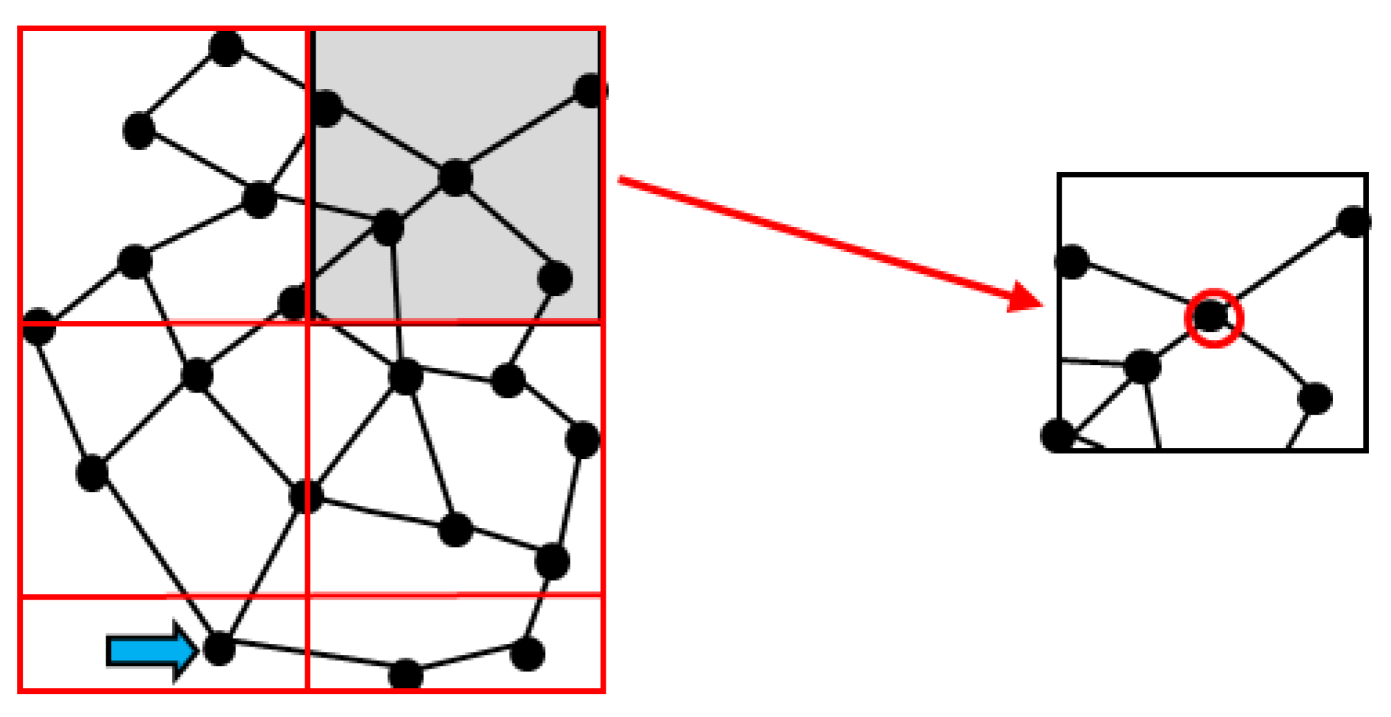
The direct application of the index W for determining the ranking of junctions in terms of their usefulness for ranking calculations would be labor-intensive. The analysis of individual junctions required each of them to be assigned the type of recipient and type of building. These data are often missing in the resources of water utilities, which does not allow for process automation. When using nodes to locate measuring points there is often a situation in which the location indications of sensors embrace adjacent nodes. The use of subareas, instead of nodes, in the first approximation of the location method eliminates this problem. In order to minimize the amount of work, the fact that the geometric structures of water supply networks meet the requirements for fractal sets in which the particular regions—distinguished depending on the employed observation scale—exhibit self-similarity, was taken into account [46]. At the first stage of the work, the area of the water supply network was divided into identical subareas—squares (see Figure 1 on the left-hand side). Such division is often used in the process of calculating the fractal dimensions of sets with the box counting method [47,48]. In the paper, the edge length of the square was assumed as equal to the distance the water in the considered network travels over six hours, with the weighted average flow rate determined at the hour of moderate water demand obtained in the simulation studies based on a numerical model. The six hours flow period was most appropriate in the previous trials [17] performed for looped-branched networks of high complexity.

The significance index W was determined for each of the designated subareas, based on the total water demand in the area and the highest—according to Table 1—type of recipients and buildings. The values of coefficient (c) were determined on the basis of the simulation studies, depending on the average concentration in a given subarea. The calculations omitted the values corresponding to the hydrant junctions. This stage was finished by indicating five subareas with the highest values of index W. The number of indicated subareas was recommended by the local water and sewerage company in which the presented method was tested. The place in the ranking simultaneously corresponded to the recommended sequence of sensor installation.

In the second stage, the process of ranking calculations was conducted in an analogous way; however, it only involved the junctions found separately in each of the previously designated subareas (Figure 2, right-hand side). It corresponds to the process of changing the observation scale in the description of fractal sets.

2.1. Comparison of Placement Indications with the Results Obtained Using Other Heuristic Methods

The locations of measurement points obtained using the method presented above were compared with the spots indicated by two other heuristic methods. The first of them, proposed by Ghimre and Barkdoll [14,15], is based on the water demand ranking in particular junctions as the sole criterion. The placement was determined using the base demand value attributed to particular junctions in the created numerical model of the considered water supply network. Preparation of the ranking required only sorting the values from the report generated as a table using the EPANET 2.0 software.

The other method employed for comparison is based on the assumption that the chlorine measurement locations should be found in the most critical locations, corresponding to the greatest water age [49,50]. The water age was determined through the simulations based on the numerical model of the considered water supply network built using the EPANET 2.0 software. The ranking omitted the dead ends and hydrant junctions.

The number of residents outside the monitoring system for the residue chlorine content in the supplied water was assumed as the first indicator, enabling the determined sensor locations to be compared using all the aforementioned methods. It was assumed that such recipients are found beyond the furthest sensor locations, taking into account the water flow directions. This number was calculated using the following formula:

$$M=\frac{{\displaystyle \sum }{Q}_S}{Q_M},$$

(2)

where ∑Q_S—total daily water demand in the subareas found beyond the monitoring locations, taking into account the water flow direction, Q_M—daily water demand per individual, calculated as the quotient of total daily water demand for the entire network and the number of residents being supplied with water.

The comparative calculations assumed that the higher the number M, the worse the location of the monitoring points.

The second criterion was based on the simulation results of water age carried out using the numerical model of the network analyzed, built in the EPANET program. The highest water age of all five locations was calculated for each method. In comparative calculations, it was assumed that the higher the h value, the longer the detection time of insufficient chlorine concentration. This corresponds to the longer exposure time of recipients to the water with impaired quality. Taking this into account, it was assumed that the higher the age expressed by the index h, the worse the location indication of the measuring points.

2.2. Analyzed Water Network

The research object was an existing water supply network, supplying a city with the population of about 50,000. The network is supplied from a single station. The covered area approximates 50.6 km². The total length of pipes, made of various materials (steel, cast iron, ductile iron, PVC (Polivinylchloride), PE (Poliethylene) and A-C (Asebestos-cement)) is roughly 270 km. The mean daily water consumption is approximately 6400 m³/d, which corresponds to 128 dm³/d per resident. The water fed into the network is disinfected with chlorine gas at the entrance to the retention tanks located at the water supply station.

A numerical model reflecting the hydraulic flow conditions and changes in water quality—concentration of residual chlorine—was built for this network using the EPANET 2.0 software. The model comprises approximately 2800 junctions and 2900 pipes. The geometric structure of the network reflected in the model is presented in Figure 2. Structurally, it is a mixed system containing both branches and over 50 loops. This figure also shows the grid of subareas (squares) employed in the first stage of the proposed method for determining the location of residual chlorine measurement points and location of chlorine measurement during the calibration process.

A first-order model in the form of an equation comprising the bulk and wall chlorine decay coefficients was employed in the calculations [44,51,52]:

C_e = C₀·e^−kt,

(3)

where C₀—initial chlorine concentration, Ce—the concentration at time t, k—decay coefficient, calculated as:

k = k_b + k_w,

(4)

k_b—bulk decay coefficient, k_w—wall decay coefficient.

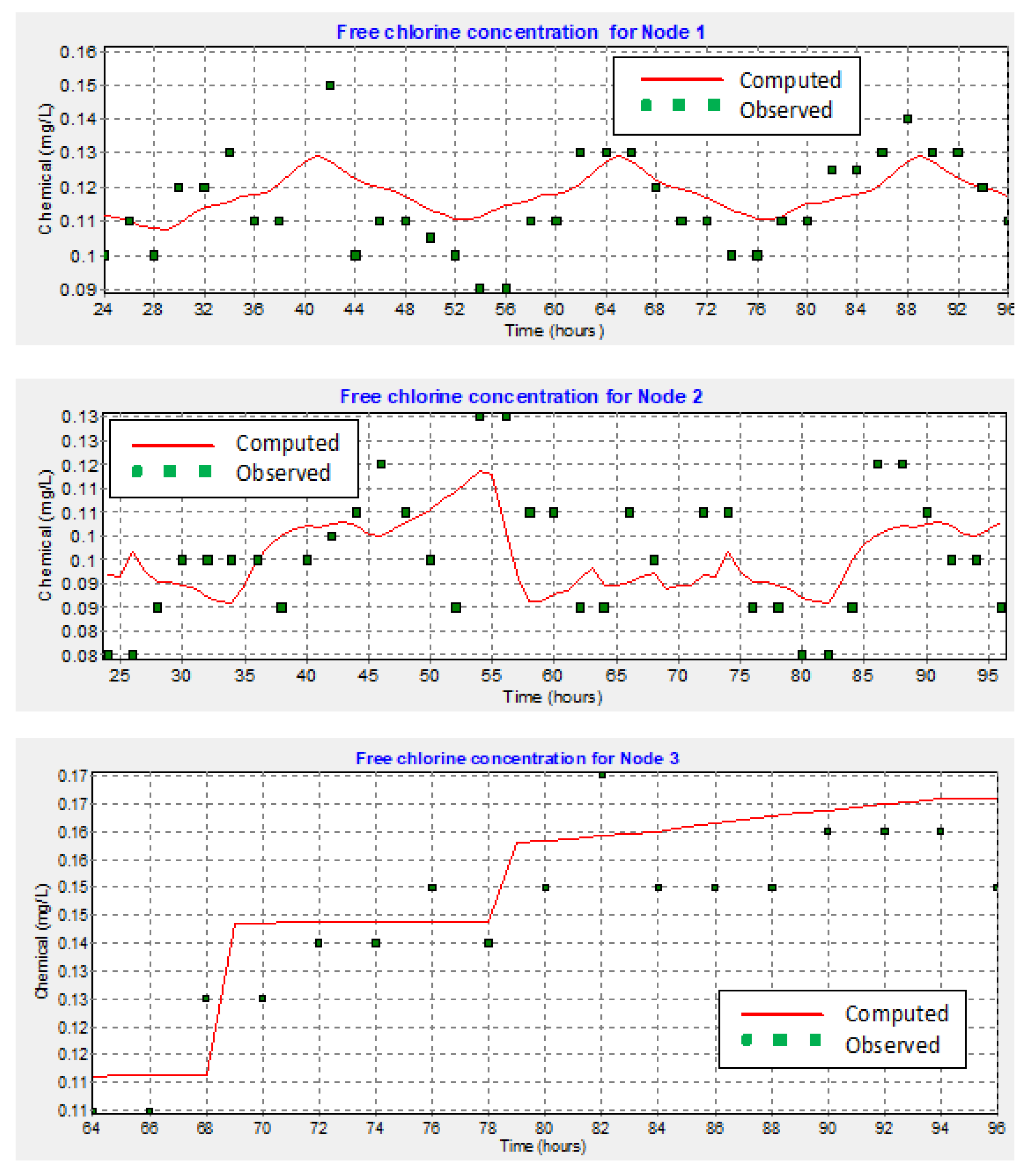
The bulk coefficient was measured in a laboratory using a bottle test and reached 0.18 1/h. In turn, the wall decay coefficient was determined in the course of the calibration calculations and ranged from 0.05 to 2.5 1/h. The results of calibration reported by EPANET are presented in

Table 3. Calibration statistics for chlorine concentration (EPANET).

Location	Number of Observed Data	Observed Mean	Computed Mean	Mean Error	RMS Error
Network	425	0.14	0.13	0.017	0.033
Correlation between means: 0.874

. The exemplary graphs showing the results of measurements and calculations of residual chlorine are shown in Figure 3. Different time values on the horizontal axes of the charts (Figure 3) result from the age of the water at the analyzed points.

3. Results and Discussion

Using the data pertaining to the water demand allocated to particular junctions, the results of simulations conducted using a numerical model and the information gathered through consultations with the employees of the local Water and Sewerage Company pertaining to the type of recipients and buildings, the location of residual chlorine measurement points was determined.

Table 4. Total water demand (m³/d) in particular subareas. The designations are in line with the ones used in Figure 2. The blue color corresponds to the water station

	A	B	C	D	E	F	G	H	I	J	K	L	M	N
1	19
2		2
3			92
4			1
5			12	94
6			0	3	3
7			6	28
8			26	17
9			64
10			112							2
11			49					20	51	6
12			132	28	82	123	95	114	673	113
13			42	419	191	271	263	249	222	38	25
14			8	239	120	103	60	262	301	53	22	21	8
15			13	5	51	37	40	513	106	33	23	28	17
16						6	45	66	79	7	9	13	14	85
17							38	30	8
18							32	34
19							14	50
20							6	29	2
21								16	3
22									3
23									2	8
24										29

presents the total daily water demand in particular subareas. The maximum value reached 673 m³/d (J12 square). The location of the pumping station, where the first measurement point was established, was marked in blue.

Table 5. Values of coefficient (Q) describing the water demand in particular subareas, (a) denoting the required reliability of water supply to particular subareas, (b) corresponding to the failure to supply water of adequate quality to particular subareas and coefficient (c) denoting the concentration of free chlorine in particular subareas.

Q Coefficient															a Coefficient
	A	B	C	D	E	F	G	H	I	J	K	L	M	N	A	B	C	D	E	F	G	H	I	J	K	L	M	N
1	1														1
2		1														1
3			1														1
4			1														1
5			1	1													1	1	1
6			1	1	1												1	1	5	1
7			1	1													1	1
8			1	1													1	1
9			1														1
10			1							1							2							1
11			1					1	1	1							3					2	1	1
12			2	1	1	1	1	1	5	1							3	2	2	1	5	2	1	1
13			1	4	2	3	2	2	2	1	1						1	2	2	4	1	3	1	1	4
14			1	2	1	1	1	2	3	1	1	1	1				1	2	3	3	3	2	1	3	2	4	4
15			1	1	1	1	1	4	1	1	1	1	1				1	1	1	2	2	1	5	1	1	2	1
16						1	1	1	1	1	1	1	1	1						2	2	1	1	1	1	1	1	1
17							1	1	1												1	1	1
18							1	1													1	1
19							1	1													2	1
20							1	1	1												1	4	1
21								1	1													1	1
22									1														1
23									1	1													1	1
24										1														1
				b Coefficient															c Coefficient
1	1														3
2		1														3
3			1														3
4			1														3
5			1	1	1												3	3	1
6			1	1	4	1											3	3	1	1
7			1	1													3	3
8			1	1													3	3
9			2														3
10			2							1							3							3
11			2					2	2	1							3					3	3	3
12			2	2	2	1	5	2	2	1							3	3	3	3	3	2	3	3
13			2	2	2	4	2	2	2	1	2						3	3	3	3	2	2	3	3	3
14			2	2	2	3	2	3	2	4	2	4	4				3	3	3	2	2	2	3	3	3	3	3
15			1	2	2	2	3	3	3	1	1	2	1				3	3	3	2	1	1	1	3	3	3	3
16						2	3	3	3	1	1	1	1	1						2	1	1	2	3	3	3	3	3
17							2	1	1												1	1	3
18							1	1													1	1	0
19							1	1													2	2	0
20							1	4	1												2	3	3
21								1	1													2	3
22									1														2
23									1	1													2	2
24										1														2

presents the calculated coefficient Q values denoting the water demand in particular subareas and shows the values of coefficients describing the required water supply reliability (a), impact related to the lack thereof (b), and the calculated chlorine concentration (c). The values of the ranking index W calculated for particular subareas are presented in

Table 6. Values of ranking index W calculated for particular subareas. The location of the pumping station was marked in blue. The red color indicates the subareas with the highest value of index W. The yellow color indicates the subareas with the next and equal value of this index.

	A	B	C	D	E	F	G	H	I	J	K	L	M	N
1	3
2		3
3			3
4			3
5			3	3
6			3	3	20
7			3	3
8			3	3
9			6
10			12							3
11			18					12	6	3
12			36	12	12	3	75	8	30	3
13			6	48	24	144	8	24	12	3	24
14			6	24	18	18	12	24	18	36	12	48	48
15			3	6	6	8	6	12	15	3	3	12	3
16						8	6	3	6	3	3	3	3	3
17							2	1	3
18							1	1
19							4	2
20							2	48	3
21								2	3
22									2
23									2	2
24										2

.

Table 7. Subareas with the highest ranking positions received by three analyzed methods.

Sensor Placement, Ranking Position	W Index Method	Maximum Water Demand Method	Maximum Water Age Method
1	F13	I12	F5
2	G12	G15	L14
3	D13	D13	J24
4	H20	G14	J10
5	L14	D14	L16

presents five subareas with the highest significance index W. Due to the situation where the values of this index is repeated, it was necessary to account for the total water demand from Table 3 to determine their order in the ranking. Assuming the location of five measurement points as the result, the M14 subarea was omitted in further considerations. In the second stage of the work, the calculation of the significance index within each of the five selected subareas was repeated. As a result, a single junction per subarea was determined as the location of measurement points. The location of these points was presented in Figure 4.

The indicated chlorine measuring the locations obtained with the W index method (red color) were compared with the locations obtained using the methods based on the ranking of junctions in terms of the water demand (blue color) and in terms of the water age (yellow)—Figure 4.

While comparing the locations of measurement points presented in Figure 4 and Table 7, it can be stated that a repetition occurred only in two cases—location no. 3 (W index and max demand method) and location no. 5 and 3 (W index and max age method, respectively).

Further on, the approximated number of residents outside monitoring M and maximum water age in the designated measurement points were compared (

Table 8. Approximate number of residents outside the monitoring of free chlorine and maximum water age for the designated measurement points.

Method	Number of Residents Outside Monitoring, M	Maximum Water Age, h
Significance index W	12,433	26.0
According to base demand	15,800	11.0
According to water age	3406	96.0

).

The indication of sensor locations based on water age as the sole parameter leads to the situation where the lowest number of residents is supplied with nonmonitored water. Unfortunately, the water age in the designated measurement points reaches the value of 96 h. This means that in extreme cases, the water company will be able to react only after four days of supplying water with insufficient chlorine concentration.

The sensor locations determined on the basis of maximum water demand as the only parameter enables obtaining the lowest maximum water age in the measurement points; however, the number of residents outside the monitoring system is the highest.

Considering the results of the calculations contained in Table 7, it should be stated that the solution based on the W index, as a compromise, has both advantages and disadvantages over the methods based on single criteria of water age and water demand. The number of residents outside the monitoring system is lower than in the base demand method by about 21%. However, the maximum water age is approximately 2.3-fold greater, in comparison to it. Nevertheless, it is significantly lower (by about 73%) than in the method based solely on the water age. In theory, it is possible to introduce the weight of the contribution of Q, a, b, and c to the W index calculation. It would probably enable achieving different optima based on the requirements of water system managers.

The application of the proposed heuristic method based on the index W turned out to be possible in an existing water supply network. The application of a two-stage process for determining the residual chlorine sensors significantly reduced the required effort. Employing different observation scales, characteristic for fractal geometry makes the investigated method versatile and enables its application in other water supply networks.

4. Conclusions

The issue of indicating a correct location for residual chlorine sensors in the water transmitted via a water supply network still remains unsolved and requires further studies.

The proposed method based on the significance index W is relatively intuitive and easy to apply by the employees of water supply and sewerage companies. However, it requires devising a numerical model reflecting both the hydraulic conditions and qualitative changes of the supplied water, as well as sound knowledge on the supplied recipients.

The comparison of three methods: Significance index W, base demand, and water age, indicates that each of them is characterized by certain limitations. However, the obtained results indicate that the proposed method enables a rational reaction of a water supply and sewerage company in emergencies, simultaneously covering a vast majority of recipients with a monitoring system.

The method proposed in the paper may be employed at an initial stage of the monitoring system design, when the number of sensors is lower than that of selected subareas. If the financial capabilities of water companies permit the gradual installation of a greater number of sensors in subsequent stages of designing the monitoring system, the size of subareas can be reduced, increasing their number.

References

- Hart, W.E.; Murray, R. Review of Sensor Placement Strategies for Contamination Warning Systems in Drinking Water Distribution Systems. J. Water Resour. Plan. Manag. 2010, 136, 611–619. [Google Scholar] [CrossRef]
- Rathi, S.; Gupta, R. Monitoring stations in water distribution systems to detect contamination events. ISH J. Hydraulic Eng. 2013. [Google Scholar] [CrossRef]
- Rathi, S.; Gupta, R. A Simple sensor placement approach for regular monitoring and contamination detection in water distribution networks. KSCE J. Civ. Eng. 2016, 20, 597–608. [Google Scholar] [CrossRef]
- Rathi, S.; Gupta, R.; Ormsbee, L. A review of sensor placement objective metrics for contamination detection in water distribution networks. Water Supply 2015, 15, 898–917. [Google Scholar] [CrossRef]
- Lee, B.; Deininger, R. Optimal locations of monitoring stations in water distribution system. ACSE J. Environ. Eng. 1992, 118, 4–16. [Google Scholar] [CrossRef]
- Kumar, A.; Kansal, M.L.; Arora, G.; Ostfeld, A.; Kessler, A. Detecting accidental contaminations in municipial water networks. J. Water Resour. Plan. Manag. 1999, 125, 308–310. [Google Scholar] [CrossRef]
- Al-Zahrani, M.A.; Moeid, K. Locating optimum water quality monitoring stations in water distribution system. ASCE World Water Environ. Resour. Congr. 2001, 393–402. [Google Scholar]
- Al-Zahrani, M.A.; Moeid, K. Optimizing water quality monitoring stations using genetic algorithms. Arab. J. Sci. Eng. 2003, 28, 57–75. [Google Scholar]
- Harmant, P.; Nace, A.; Kiene, L.; Fotoohi, F. Optimal supervision of drinking water distribution network. In Proceedings of the ASCE 29th Annual Water Resources Planning and Management Conference, Tempe, AZ, USA, 6–9 June 1999; pp. 52–60. [Google Scholar]
- Tryby, M.E.; Uber, J.G. Representative Water Quality Sampling in Water Distribution Systems. In Proceedings of the World Water and Environmental Resources Congress, Orlando, FL, USA, 20–24 May 2001. [Google Scholar]
- Woo, H.M.; Yoon, J.H.; Choi, D.Y. Optimal monitoring sites based on water quality and quantity in water distribution systems. In Proceedings of the ASCE World Water and Environmental Resources Congress, Orlando, FL, USA, 20–24 May 2001; pp. 397–405. [Google Scholar]
- Liu, S.; Liu, W.; Chen, J.; Wang, Q. Optimal locations of monitoring stations in water distribution systems under multiple demand patterns: A flaw of demand coverage method and modification. Front Environ. Sci. Engin. China 2011. [Google Scholar] [CrossRef]
- Kansal, M.L.; Dorji, T.; Chandniha, S.K. Design Scheme for water quality monitoring in a distribution network, International. J. Environ. Dev. 2012, 9, 69–81. [Google Scholar]
- Ghimire, S.R.; Barkdoll, B.D. Heuristic method for the battle of the water network sensors: Demand-based approach. In Proceedings of the 8th Annual Water Distribution System Analysis Symposium, Cincinnati, OH, USA, 27–30 August 2006. [Google Scholar]
- Ghimire, S.R.; Barkdoll, B.D. A heuristic method for water quality sensor location in a municipal water distribution system: Mass related based approach. In Proceedings of the 8th Annual Water Distribution System Analysis Symposium, Cincinnati, OH, USA, 27–30 August 2006. [Google Scholar]
- Xu, J.H.; Fischbeck, P.S.; Small, M.J.; VanBriesen, J.M.; Casman, E. Identifying sets of key nodes for placing sensors in dynamic water distribution networks. J. Water Resour. Plan. Manag. 2008, 134, 378–385. [Google Scholar] [CrossRef]
- Kowalski, D.; Kowalska, B.; Kwietniewski, M. Localisation method of water quality measurement points in Pulawy water network monitoring system. Ochrona Środowiska 2013, 35, 45–48. [Google Scholar]
- Kowalski, D.; Kowalska, B.; Kwietniewski, M. Monitoring of water distribution system effectiveness using fractal geometry. Bull. Pol. Acad. Sci. Tech. Sci. 2015, 63, 155–161. [Google Scholar] [CrossRef] [Green Version]
- Kowalski, D.; Kowalska, B.; Kwietniewski, M.; Duklewski, W.; Dziak, S.; Czajka, S.; Mierzwa, A. Method for determining the location of water quality sensors in water supply networks. Pol. Pat. 2015, 63, 155–161. [Google Scholar]
- Kessler, A.; Ostfeld, A.; Sinai, G. Detecting accidental contaminations in municipal water networks. J. Water Resour. Plan. Manag. 1998, 124, 192–198. [Google Scholar] [CrossRef]
- Ostfeld, A.; Salomons, E. Optimal layout of early warning detection stations for water distribution systems security. J. Water Resour. Plan. Manag. 2004, 130, 377–385. [Google Scholar] [CrossRef]
- Zhao, Y.; Schwartz, R.; Salomons, E.; Ostfeld, A.; Poor, H.V. New formulation and optimization methods for water sensor placement. Environ. Model. Softw. 2016, 76, 128–136. [Google Scholar] [CrossRef]
- Cozzolino, L.; Mucherino, C.; Pianese, D.; Pirozzi, F. Positioning, within water distribution networks, of monitoring stations aiming at an early detection of intentional contamination. Civ. Eng. Environ. Syst. 2006, 23, 161–174. [Google Scholar] [CrossRef]
- Berry, J.W.; Boman, E.; Phillips, C.A.; Riesen, L.A. Low-memory Lagrangian Relaxation Methods for Sensor Placment in Municipal Water Networks. In Proceedings of the Word Environmental and Water Recources Congress, ASCE, Reston, VA, USA, 17–21 May 2008. [Google Scholar]
- Berry, J.W.; Boman, E.; Phillips, C.A.; Riesen, L.A. User’s Manual: Teva-Spot Toolkit 2.0.; Sandia National Laboratories: Albuquerque, NM, USA, 2008. [Google Scholar]
- Hart, W.E.; Berry, J.W.; Boman, E.G.; Murray, R.; Phillips, C.A.; Riesen, L.A.; Watson, J.P. The TEVA-SPOT toolkit for drinking water contaminant warning system design. In Proceedings of the World Environmental & Water Resources Congress, ASCE, Reston, VA, USA, 17–21 May 2008. [Google Scholar]
- Ostfeld, A.; Salomons, E. Optimal early warning monitoring system layout for water networks security: Inclusion of sensors sensitivities and response delays. Civ. Eng. Environ. Syst. 2005, 22, 151–169. [Google Scholar] [CrossRef]
- Ostfeld, A.; Salomons, E. Securing water distribution systems using online contamination monitoring. J. Water Resour. Plan. Manag. 2005, 131, 402–405. [Google Scholar] [CrossRef]
- Łagnowski, R.; Brdys, M.A. An optimised placement of the hard quality sensors for a robust monitoring of the chlorine concentration in drinking water distribution systems. J. Process Control 2018, 68, 52–63. [Google Scholar]
- Clark, R.M. Chlorine demand and TTHM formation kinetics: A second—Order model. J. Environ. Eng. 1998, 124, 16–24. [Google Scholar] [CrossRef]
- Kowalska, B.; Kowalski, D.; Musz, A. Chlorine Decay in Water Distribution System. Environ. Prot. Eng. 2006, 32, 5–16. [Google Scholar]
- Al Heboos, S.; Licskó, I. Influence of water quality characters on kinetics of chlorine bulk decay in water distribution systems. Int. J. Appl. Sci. Technol. 2015, 5, 64–73. [Google Scholar]
- Al-Jasser, A.O. Chlorine decay in drinking-water transmission and distribution systems: Pipe service age effect. Water Res. 2007, 41, 387–396. [Google Scholar] [CrossRef]
- Courtis, B.J.; West, J.R.; Bridgeman, J. Temporal and spatial variations in bulk chlorine decay within a water supply system. J. Environ. Eng. 2009, 135, 147–152. [Google Scholar] [CrossRef]
- Kowalska, B.; Hołota, E.; Kowalski, D. Simulation of chlorine concentration changes in a real water supply network using EPANET 2.0 and WaterGEMS software. WIT Trans. Built Environ. 2018, 184, 39–48. [Google Scholar]
- Castro, P.; Neves, M. Chlorine decay in water distribution systems. Case study—Lousada network. Electron. J. Environ. Agric. Food Chem. 2003, 2, 261–266. [Google Scholar]
- Al-Zahrani, M.A. Optimizing Dosage and Location of Chlorine Injection in Water Supply Networks. Arab. J. Sci. Eng. 2016, 41, 4207–4215. [Google Scholar] [CrossRef]
- Bensoltane, M.A.; Zeghadnia, L.; Djemili, L.; Gheid, A.; Djebbar, Y. Enhancement of the free residual chlorine concentration at the ends of the water supply network: Case study of Souk Ahras city—Algeria. J. Water Land Dev. 2018, 38, 3–9. [Google Scholar] [CrossRef] [Green Version]
- Delpla, I.; Florea, M.; Pelletier, G.; Rodriguez, M.J. Optimizing disinfection by-product monitoring points in a distribution system using cluster analysis. Chemosphere 2018, 208, 512–521. [Google Scholar] [CrossRef] [PubMed]
- Brown, M.A.; Emmert, G.L. On-line monitoring of trihalomethane concentrations in drinking water distribution systems using capillary membrane sampling-gas chromatography. Anal. Chim. Acta 2006, 555, 75–83. [Google Scholar] [CrossRef]
- Asoka, J. Application of a risk management system to improve drinking water safety. J. Water Health 2008, 6, 547–557. [Google Scholar]
- Boryczko, K.; Rak, J.; Tchórzewska-Cieślak, B. Analysis of risk and failure scenarios in water supply system. J. Pol. Saf. Reliab. Assoc. Summer Saf. Reliab. Semin. 2014, 5, 35–42. [Google Scholar]
- Urbanik, M.; Tchórzewska-Cieślak, B. Approach to the determination of failure risk level index on the example of the natural gas distribution subsystem. J. Civ. Eng. Environ. Archit. JCEEA 2017, XXXIV, 305–312. [Google Scholar] [CrossRef]
- Rossman, L.A. EPANET 2. Users Manual. U.S. Patent EPA/600/R-00/057, 28 June 2000. [Google Scholar]
- Regulation of the Polish Minister of Health, 7th December 2017. Dziennik Ustaw 2017. pos. 2294.
- Kowalski, D.; Kowalska, B. Fractal classification of water supply networks. In Proceedings of the Eleventh International Conference on Computing and Control for the Water Industry Urban Water Management: Challenges and Opportunities, Exeter, UK, 5–9 September 2011; pp. 323–329. [Google Scholar]
- Falconer, K.J. Fractal Geometry: Mathematical Foundations and Applications; John Wiley: Chichester, UK, 1990. [Google Scholar]
- Peitgen, H.O.; Jurgens, H.; Sanpe, D. Chaos and Fractals: New Frontiers of Science; Springer: New York, NY, USA, 1992. [Google Scholar]
- Chen, W.J.; Weisel, C.P. Halogenated DBP concentrations in a distribution system. J. Am. Water Work. Assoc. 1998, 90, 151–163. [Google Scholar] [CrossRef]
- Rodriguez, M.J.; Sérodes, J.B.; Levallois, P.; Proulx, F. Chlorinated DBPs in drinking water according to source, treatment, season and distribution location. J. Environ. Eng. Sci. 2007, 6, 355–365. [Google Scholar] [CrossRef] [Green Version]
- Hua, F.; West, J.R.; Barker, R.A.; Forster, C.F. Modelling of chlorine decay in municipal water supplies. Water Res. 1999, 33, 2735–2746. [Google Scholar] [CrossRef]
- Hallam, N.B.; West, J.R.; Forster, C.F.; Powell, J.C.; Spencer, I. The decay of chlorine associated with the pipe wall in water disinfection systems. Water Res. 2002, 36, 3479–3488. [Google Scholar] [CrossRef]
Figure 1.
Stages of determining the sensor location. The first stage is seen on the left—division of the network into subareas. The second stage involving determination of the junction with the highest ranking position in the subarea is presented on the right. The blue arrow indicates the water supply point corresponding to the location of the first measurement point.
Figure 2.
Geometric structure of the network represented in a numerical model along with the location of exemplary free chlorine measurement points used in the calibration process and the employed grid of subareas.
Figure 3.
Exemplary graphs showing the results of field studies and simulations following the calibration process—Node 1 at the top, Node 2 in the middle, and Node 3 at the bottom. The numbers of measurement points are in accordance with Figure 2.
Figure 4.
Sensor locations indicated using the proposed ranking method based on index W (red color), maximum water demand (blue), and maximum water age (yellow).