A New Coupled Modeling Approach to Simulate Terrestrial Water Storage in Southern California

Department of Geography, San Diego State University, San Diego, CA 92182, USA
*
Author to whom correspondence should be addressed.
Water 2020, 12(3), 808; https://doi.org/10.3390/w12030808
Submission received: 31 December 2019
/
Revised: 5 March 2020
/
Accepted: 12 March 2020
/
Published: 14 March 2020
(This article belongs to the Section Hydrology)
Abstract
:The study introduces a new atmosphere-land-aquifer coupled model and evaluates terrestrial water storage (TWS) simulations for Southern California between 2007 and 2016. It also examines the relationship between precipitation, groundwater, and soil moisture anomalies for the two primary aquifer systems in the study area, namely the Coastal Basin and the Basin and Range aquifers. Two model designs are introduced, a partially-coupled model forced by reanalysis atmospheric data, and a fully-coupled model, in which the atmospheric conditions were simulated. Both models simulate the temporal variability of TWS anomaly in the study area well (R2 ≥ 0.87, P < 0.01). In general, the partially-coupled model outperformed the fully-coupled model as the latter overestimated precipitation, which compromised soil and aquifer recharge and discharge. Simulations also showed that the drought experienced in the area between 2012 and 2016 caused a decline in TWS, evapotranspiration, and runoff of approximately 24%, 65%, and 11%, and 20%, 72% and 8% over the two aquifer systems, respectively. Results indicate that the models first introduced in this study can be a useful tool to further our understanding of terrestrial water storage variability at regional scales.
1. Introduction
Terrestrial water storage (TWS) is defined as the summation of water on the land surface and in the subsurface. It includes soil moisture and groundwater, as well as water stored in vegetation and snow. The ability to estimate TWS accurately is essential for hydrological studies and water resource assessment, particularly in arid and semi-arid regions where access to rainfall-fed surface water storage is limited. These areas are particularly vulnerable to climate extremes, such as droughts, which often further deteriorate TWS through enhanced evaporative losses and increased groundwater extraction [1,2,3].
The region of Southern California, located along the west coast of North America between the latitudes 31° N and 36° N, is mainly characterized by a semi-arid and mild-winter Mediterranean climate. This region has experienced a rapid population growth over the last 50 years [4], which has continuously increased the demand for agricultural and urban water uses in the region. Unlike the central and northern parts of the state, the contribution of snowfall to Southern California’s TWS is negligible as wintertime temperatures are too warm for considerable snow to accumulate, except in a few high mountain peaks [5]. Furthermore, the local shrubland vegetation is sparsely distributed and does not hold substantial amounts of water [6]. Therefore, variations in TWS in the region are primarily driven by changes in soil moisture and groundwater contents.
Groundwater is one of the most valuable sources of freshwater in the world. Almost two billion people worldwide and fifty percent of the United States’ populations use it for drinking and irrigation [7]. Current estimates indicate that groundwater provides 38% of the total water supply for California. This rate can reach 46% or more during dry years. Moreover, in some rural locations of the state, groundwater delivers 100% of the freshwater [8]. Future climate scenarios suggest a decrease in precipitation over the next 80 years for Southern California, while projections for the end of the 21st century indicate a steady increase in population for the area [9]. These scenarios suggest that in order to sustain agricultural output and supply an increasing population with drinking water, groundwater will probably be extracted at higher rates, significantly depleting TWS in the future [10].
Estimation of TWS is also relevant in the context of wildfire management in the region. Soil moisture content is an important factor for wildfire risk assessment and prediction. Studies indicate that larger wildfires are more frequent when soil moisture is low, which suggests that the relationship between TWS and fire activity could be useful for the development of predictive capabilities [11,12]. Thus, accurate TWS estimates can potentially help local authorities and stakeholders manage fire-fighting resources and improve wildfire risk assessments.
Despite being such a valuable resource, the development of numerical models to simulate TWS, in particular groundwater variations at regional scales, has been somewhat limited. Global water balance model simulations driven by satellite-derived TWS and soil moisture retrievals have been used to generate information on changes in groundwater storage [3,13]. These studies demonstrate that merging modeling and satellite data can improve the calculation of water balance components. These techniques, however, may not be adequate for regional or local-scale applications due to the low spatial resolution of global water balance models.
Previous studies [14,15] describe some of the first attempts to explicitly calculate TWS variations based on meteorological forcing data and soil properties. These physically-based models have been implemented in more complex land and climate models to generate variations in TWS over different regions [16,17,18]. A study using the Community Land Model showed that the use of land-aquifer coupled models could reduce the uncertainty in satellite-based estimates of aquifer discharge and anthropogenic groundwater depletion [19]. Furthermore, the fusion of satellite and land model TWS estimates has also been explored as a technique to assess changes in water table depth in California [20]. That study, which uses the Variable Infiltration Capacity land model, concluded that the assimilation of satellite TWS estimates could significantly improve the model’s skill in simulating long-term trends of seasonal and interannual variability in groundwater.
Other studies such as [16,21] describe simulations using fully-coupled climate-land-aquifer regional models. Unlike land-aquifer models which are driven by either observational or analysis climate data, fully-coupled models can generate meteorological information, and thus, have the ability to simulate both past and future atmospheric and TWS scenarios. In general, these studies suggest that the implementation of TWS dynamics in climate models not only generates accurate simulations of surface and subsurface water recharge and discharge, they can also be especially beneficial for precipitation forecasts, as they improve the calculation of surface and sub-surface water available for evapotranspiration and runoff.
This study introduces a new atmosphere-land-aquifer coupled model formed by the Weather Research and Forecasting (WRF), the Simplified Simple Biosphere (SSIB), and the Simple Groundwater (SIMGM) models [15,22,23]. This is the first time these three models have been linked together to form a fully-coupled atmosphere-land-aquifer modeling system. The model was tested for a domain centered over Southern California to simulate anomalies in TWS for a period between 2007 and 2016. This period was selected because it included a prolonged drought, which affected most of the study area [24,25].
2. Models, Data, and Methods
2.1. The Atmosphere and Land Surface Models
The Weather Research and Forecasting (WRF) regional atmospheric model is an advanced, non-hydrostatic, and fully compressible regional climate model designed for both meteorological research and numerical weather prediction. It is built upon a system with terrain-following vertical and staggered Arakawa C-grid-type horizontal coordinates. The model offers several radiation, convective, and microphysics scheme options and is currently maintained and supported by the Mesoscale and Microscale Meteorology Division at the National Center for Atmospheric Research [22,26].
The third version of the Simplified Simple Biosphere (SSIB) is a biophysically-based land surface model and was used in this study to simulate the land surface-atmosphere interactions by calculating the surface energy budget and surface water balance based on three soil layers and one vegetation canopy layer [23]. In addition to simulating processes such as photosynthesis-controlled transpiration, soil evaporation, and runoff, it also includes a multi-layer snow hydrology module to realistically simulate processes associated with snow load and melting, substantially enhancing the model’s ability for soil hydrology studies [5].
2.2. The Aquifer Model
We used a modified version of the Simple Groundwater Model (SIMGM) to simulate the temporal variations of water stored in an aquifer [15]. In the SIMGM, an unconfined aquifer is defined as the portion of ground located below the soil column, and the variations of water stored in the aquifer (WA) over time are calculated as:
where Qin and Qout are the aquifer recharge and discharge (mm s−1), respectively. Qin is obtained through Darcy’s Law as:
where Kbot, Ψbot are the soil hydraulic conductivity and matric potential of the bottom soil layer; zbot is the depth of the bottom soil layer (1.5 m), and zw is the water table depth. Equation (2) accounts for downward water flux driven by gravitational drainage, as well as upward water flux driven by capillary forces.
Measurements of aquifer hydraulic conductivity are available for only a few aquifers, therefore, to avoid uncertainties in determining the aquifer’s hydraulic conductivity, the bottom soil layer’s hydraulic conductivity was used when calculating the aquifer recharge [17]. The hydraulic conductivity within the soil column in the SSIB model was determined based on the soil texture [27] and the soil matric potential was calculated based on the empirical relationships [28]. Aquifer discharge, also known as baseflow or subsurface runoff, is parameterized as:
where Qout.max is the maximum aquifer discharge, which happens when the water table is at its highest (zw = 0) and F is the subsurface runoff or baseflow decay factor. Qout.max is a function of the aquifer’s topographic aspect and the maximum saturated fraction within a grid cell and is obtained through calibrations against water table depth data since Qout.max measurements are rarely available. A value of 5 × 10⁻⁴ mm s−1 was used in this study, which was obtained through calibration against global runoff data through sensitivity tests and is described in [17].
We were aware that using a value obtained through global data calibration could introduce errors when calculating total aquifer storage; but it should be negligible when determining seasonal variations of the water table depth [15]. On the other hand, the baseflow decay factor (F) has an important role in aquifer storage anomalies, and therefore, its values must be determined through calibration against observations or remotely-sensed estimates for the study area. As shown in Section 2.7, we used satellite-based TWS anomalies to estimate this parameter.
Finally, simulated water table depth (zw) can be obtained from the aquifer water storage (Wa) scaled by the aquifer specific yield, which is the fraction of water volume that can be drained by gravity form the aquifer. While specific yield ranged from 0.02 for clay to 0.27 for sandy soil, we used the same constant value utilized in the original model development (0.2) due to the lack of specific yield data in the study [15].
2.3. Model Coupling Approaches
This study describes the implementation and results of two different model-coupling approaches. The first is a partially-coupled model consisting of the SSIB land and the SIMGM aquifer models (SSIB-SIMGM henceforth), in which the atmospheric conditions are not simulated by the model. In this approach, hourly precipitation, atmospheric pressure, downward solar and terrestrial radiation, 30-m air temperature, humidity, and wind, obtained from the North American Regional Reanalysis (NARR) were used as forcing data for the model [29]. In the second approach, the SSIB-SIMGM was implemented in WRF to form a fully-coupled atmosphere-land-aquifer regional modeling system (WRF-SSIB-SIMGM), which in addition to the surface and subsurface layers, included 38 vertical atmospheric layers. Initial and lateral-boundary atmospheric conditions for this model were also taken from the NARR dataset.
Both models were configured for a domain set up on a 10-km horizontal resolution grid extending from 31° N to 36° N and from 121.5° W to 115° W, which covered Southern California and the adjoining Atlantic Ocean (Figure 1). MODIS-derived monthly leaf area index and vegetation cover fraction maps were used in all coupled and uncoupled simulations. Preliminary short-term simulations were conducted with WRF to determine the best physics option combination for the study area, which resulted in the following selection: Ferrier microphysics scheme [30], the Fu-Liou-Gu shortwave and longwave radiation schemes [31], the Yonsei University PBL scheme [32], and the Grell-Devenyi convective scheme [33]. Furthermore, a set of five simulations were performed with the fully-coupled model, starting from slightly different atmospheric initial conditions, to minimize the effects of uncertainties associated with the initial boundary conditions and the model internal variability.
2.4. Terrestrial Water Storage Data
Global-gridded TWS estimates derived from temporal gravity field variations measured by the Gravity Recovery and Climate Experiment (GRACE) were used to validate the models [34]. GRACE TWS anomaly estimates are available at https://grace.jpl.nasa.gov [35] in three distinct datasets, each of which are obtained through different filtering and geophysical correction algorithms [36,37,38]. The data is available on a 1° × 1° latitude-longitude geographical resolution grid and represents the latest versions of GRACE estimates up to date. We utilized the average of all three datasets to calibrate the model’s baseflow decay factor (Section 2.7) and to assess the model’s TWS simulation performance. The use of GRACE estimates for modeling validation purposes has been employed in several studies [15,17,18,39].
2.5. Model Domain
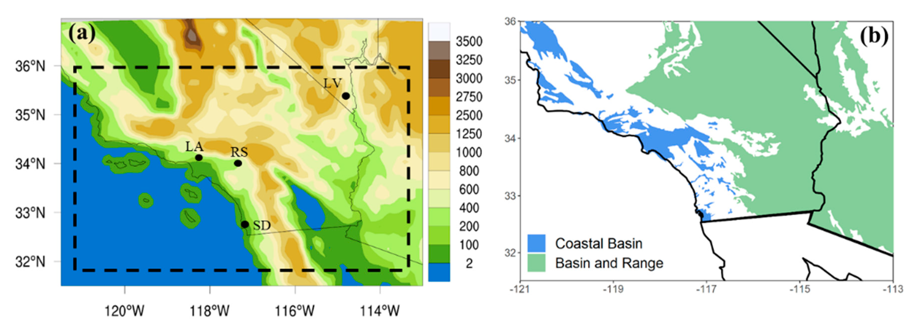
The model domain used for the validation was bounded by 31.5° N and 36° N, and 125° W and 113.5° W (Figure 1a). This area is characterized by Mediterranean, semi-arid, and desert climate types with warm, dry summers and cool, wet winters. Coastal regions are enclosed by mountain ranges and strongly influenced by maritime air masses. Precipitation peaks in the winter with variable snow accumulation in the higher terrain. Many large metropolitan areas lie in this section of the domain including Los Angeles and San Diego.
The interior portions of the domain are much drier and warmer with mostly semi-arid and arid climates. Precipitation is also greater in the winter months, but the North American monsoon occasionally brings rainfall to the region in the summer and early fall. The study area features two main aquifer systems namely the Coastal Basin aquifers located along the coast and the Basin and Range aquifers located inland (Figure 1b). Despite having different geohydrologic settings, geologic history, and land- and water-use characteristics, both aquifer systems are used to supplement water supply at different rates [40].
2.6. Terrestrial Water Initial Conditions
A spin-up approach was utilized to generate initial conditions of soil moisture and groundwater over the study area. In this approach, aquifer storage is started from an arbitrary value and the model run repeatedly through one year until the domain-average aquifer storage reaches equilibrium [18], which occurs when:
where represents the domain-average aquifer water storage, and n indicates a day in the simulation. For this study, the aquifers were initialized as completely full throughout the domain; and repeated simulations were performed for the period between November 2004 and October 2005 using NARR as the forcing data and a globally-calibrated baseflow decay factor of 6.0 m−1 [17].
Results showed that the average aquifer storage reached equilibrium at n = 9000 days of simulation, or approximately after 24.6 years. Results from this spin-up were used to initialize both aquifer and soil moisture conditions for all simulations described hereafter. Furthermore, it should be noted that in addition to the spin-up run to generate soil and subsurface initial conditions, both models (SSIB-SIMGM and WRF-SSIB-SIMGM) were allowed one additional year (November 2006 to October 2007) of spin-up to guarantee consistency between soil and atmospheric initial conditions.
2.7. Baseflow Decay Factor Calibration
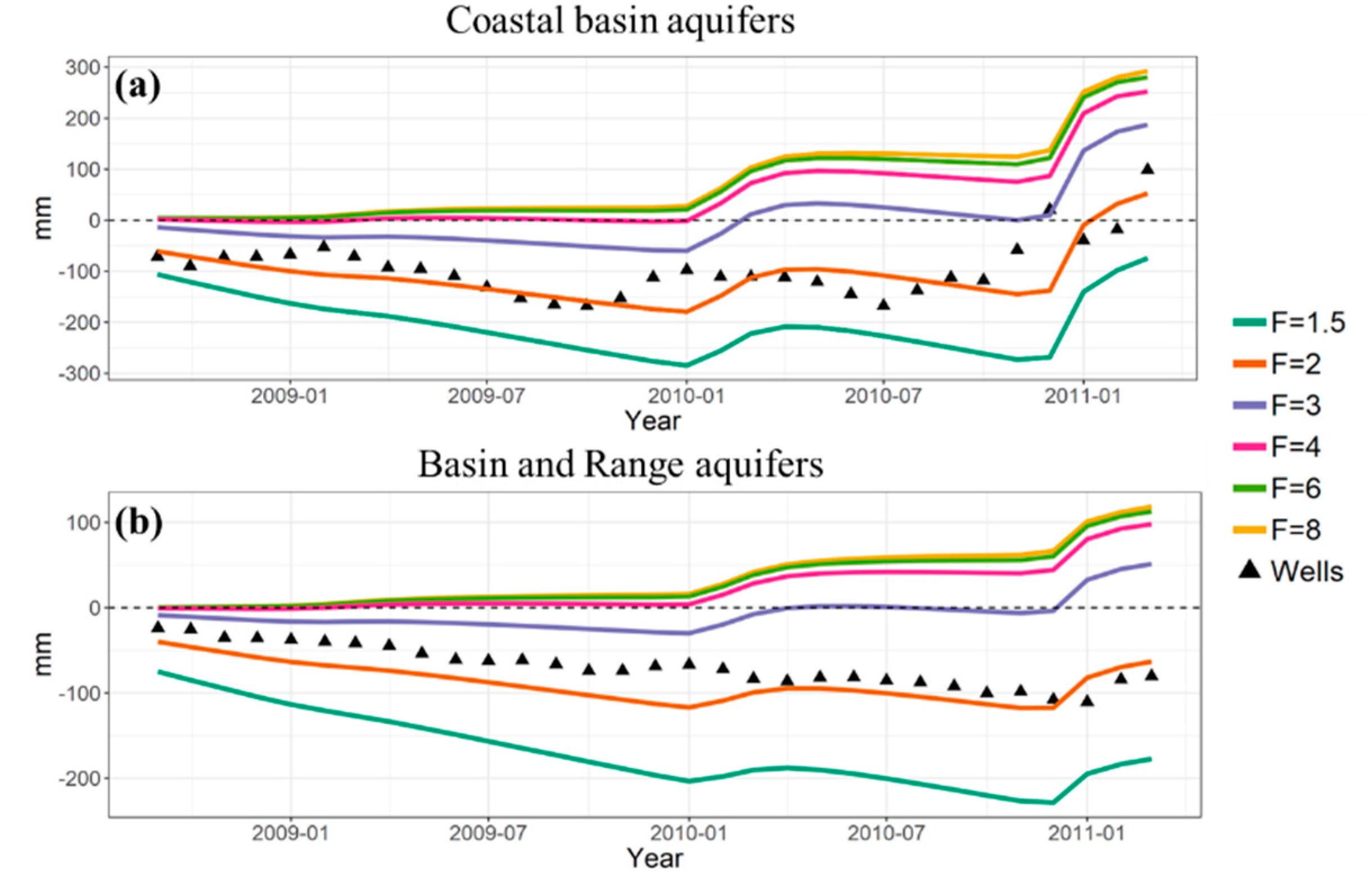
The baseflow decay factor (F) of an aquifer has an important role in determining terrestrial water storage. Due to the lack of observational data, the baseflow decay factor must be defined through calibration with remotely-sensed data. Previous studies show F values ranging from 1.25 to 8 m−1 [14,15,17]. We determined the optimum baseflow decay factor for two aquifer systems in our study area by performing partially-coupled model simulations for F values ranging from 1 to 8 m−1 and comparing simulated water table depth anomalies against measurements from 59 United States Geological Survey wells (Table S1).
Table 1 summarizes the impact of the factor in the simulated water depth anomalies for the two main aquifer systems in the study area. Despite underestimating the water table decline in some months, simulations using a decay factor equal to 2 m−1 yielded the best results for both aquifer systems, with an average root-mean-square error (RMSE) of 4.6 mm for the Basin and Range aquifer system and 9.5 mm for the Coastal Basin aquifer system (Figure 2 and Table 1). Therefore, this value was used in all subsequent simulations described in this study. This value was also similar to baseflow decay factors used in other similar studies [14,15].
3. Results
This section describes the 10-year simulations (2007–2016) for both modeling approaches. GRACE estimates were used to assess the model’s performance in terms of TWS simulations. All anomalies were calculated based on the 2007–2010 average baseline. We started by examining the results from the partially-coupled (SSIB-SIMGM) model.
3.1. SSIB-SIMGM Model
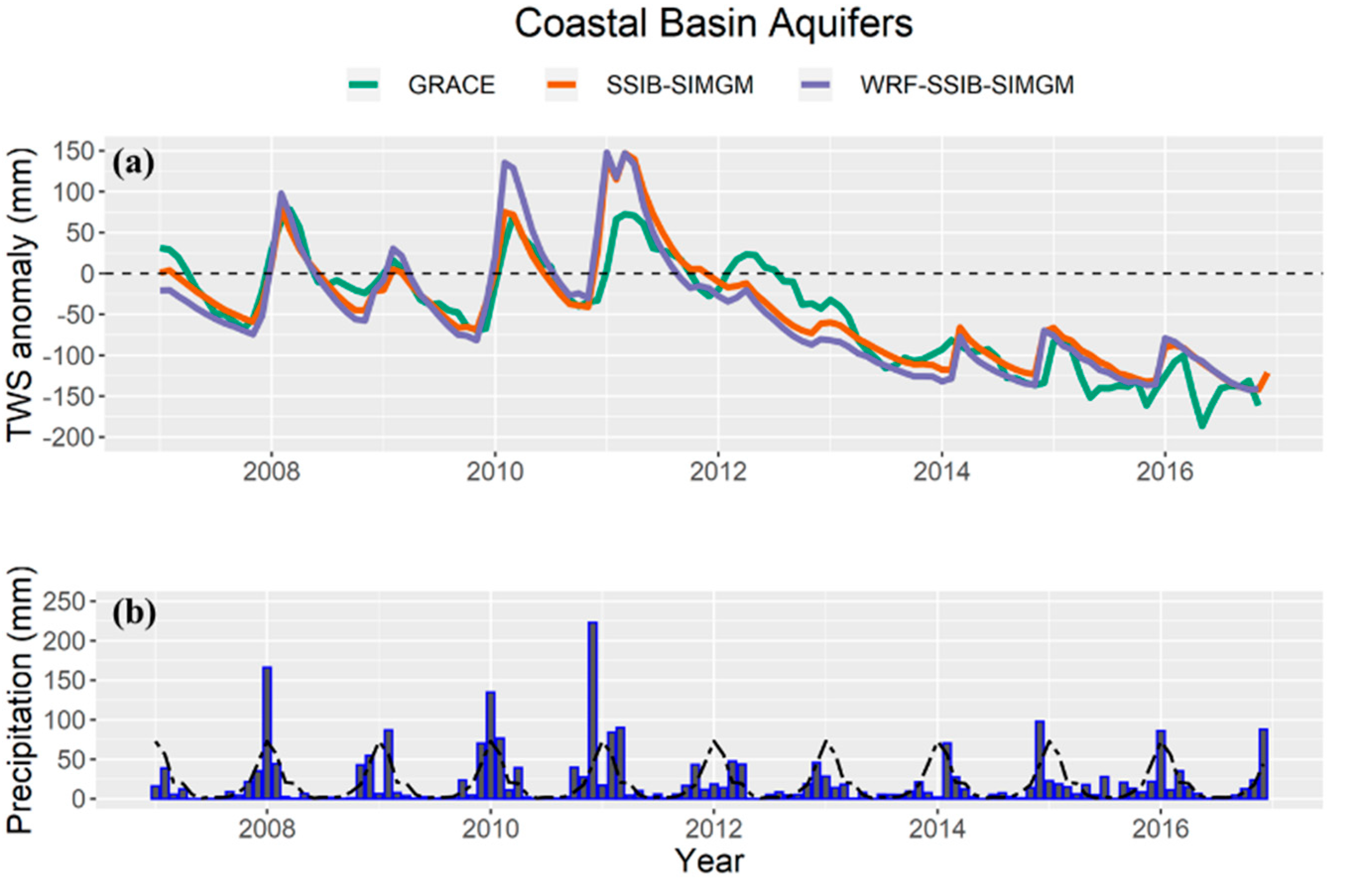
As previously described, atmospheric conditions and precipitation were not simulated in this model, rather, they were introduced as forcing data. Figure 3 and Figure 4 show GRACE and modeled monthly TWS anomaly and mean precipitation averaged over the Coastal Basin and Basin and Range aquifer systems, respectively. In general, the model was able to capture the annual cycle of dry-season discharge and wet-season recharge of TWS in the study area. Temporal correlation between GRACE and SSIB-SIMGM modeled TWS anomalies for the two aquifer systems were 0.90 and 0.94, respectively. Both coefficients were significant at a 99.9% confidence interval (Table 2).
In the first four years of the simulation, the model performed well for the Coastal Basin aquifers and captured the amplitude of the recharge-discharge annual cycle. However, it overestimated the TWS anomaly in 2011. A closer look at the monthly precipitation showed that December 2010 was an unusually wet month in coastal Southern California. Approximately 220.0 mm fell over the aquifer system that month, which was about five times the average rainfall in December for the area (44.1 mm month−1), making it the wettest December in 121 years for the Los Angeles metropolitan area. On average, the 2010−2011 rainy season received 74.3 mm of precipitation or about twice the average for the region. The above-average precipitation resulted in excessive TWS recharge for the coastal aquifers, which was overestimated by both models.
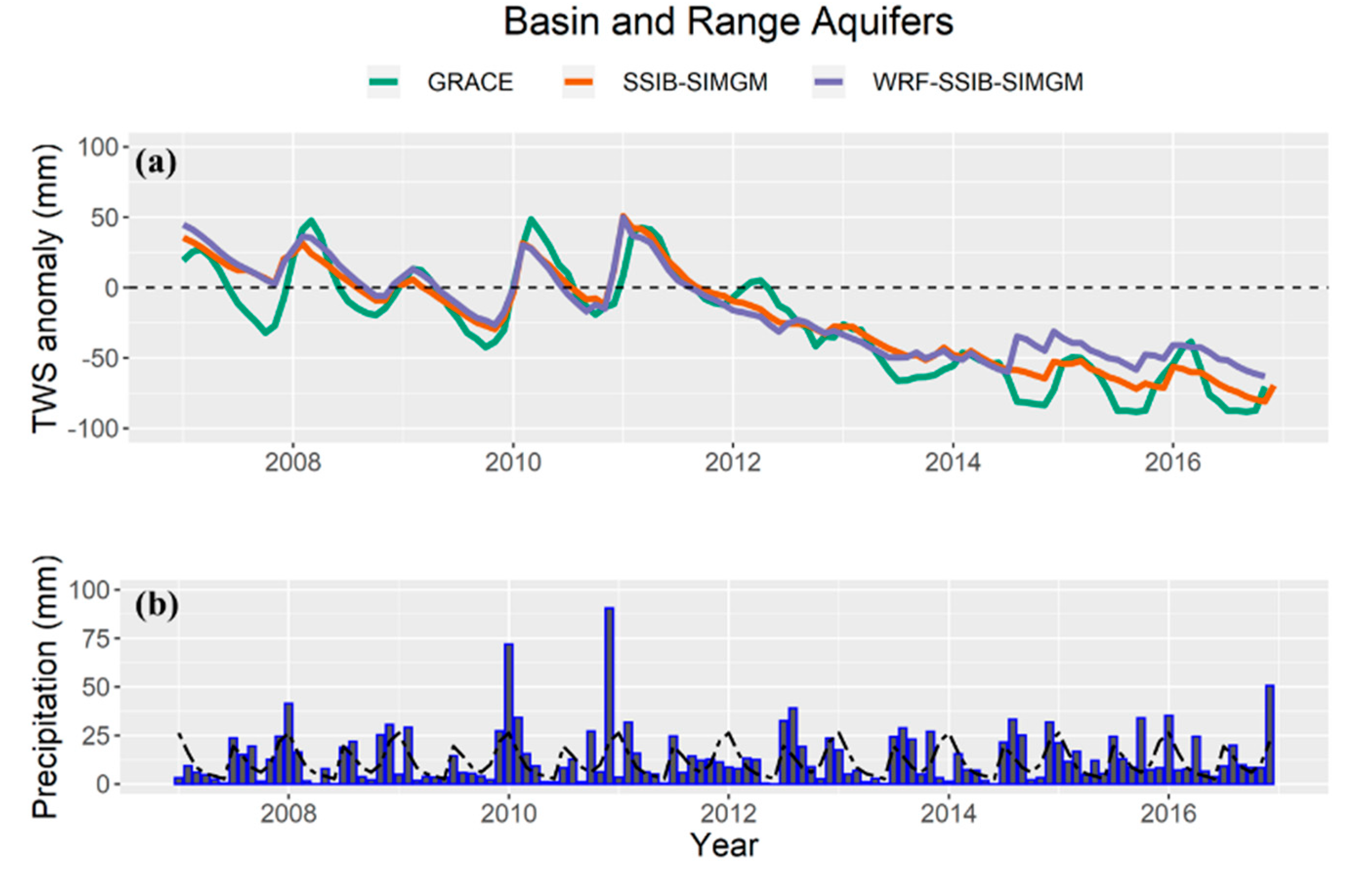
On the other hand, the model underestimated the amplitude of TWS anomalies in the Basin and Range aquifer system between 2007 and 2010 (Figure 4a). This was particularly evident in 2007 when the model missed the negative anomalies by the end of year. The large wet bias simulated in 2011 in the Coastal Basin aquifer was not seen in the Basin and Range aquifers, despite the above-average rainfall observed in both aquifers.
The year 2012 signaled the start of a steady decline in TWS for both aquifer systems, which continued until the end of the simulation. This decline was associated with a long drought observed in Southern California [24,25]. During those years, precipitation is well below the climatological averages throughout the region (Figure 3b and Figure 4b). Despite simulating the prolonged drying of the aquifer, the model underestimated its magnitude, especially in the last two years of simulation, when GRACE registered its largest TWS decline values (Figure 3a and Figure 4a). The SSIB-SIMGM model biases were more severe in the Basin and Range aquifers, and particularly large during the dry season when discharge is dominant. These results suggest that, during the drought, the model underestimated the baseflow discharge. The implementation of variable baseflow discharge factor could perhaps improve simulations under severe drought conditions.
The 10-year average bias between modeled and GRACE TWS anomalies for the aquifer systems were approximately 3.8 mm and 6.3 mm month−1 (Table 2). It should be noted that the GRACE estimates included groundwater withdrawal for irrigation and commercial use. These processes were not implemented in the models, which could amplify the model biases during the drought years in some locations.
To further assess the model’s performance, we evaluated the average time lag between precipitation and TWS response peaks for both aquifer systems. TWS response time provides crucial insight about the model’s ability to simulate important interactive mechanisms between the region’s climate and hydrology, which may not be well represented in the model. The response time was obtained by calculating the correlation coefficients between GRACE and model TWS anomalies and precipitation for different monthly time lags, and identifying the lag corresponding to the maximum correlation coefficient [41,42]. While GRACE TWS anomalies peaked two months after precipitation in both aquifer systems, modeled TWS anomalies peaked one month after precipitation. Further investigation of the model dynamics are necessary to explain this behavior.
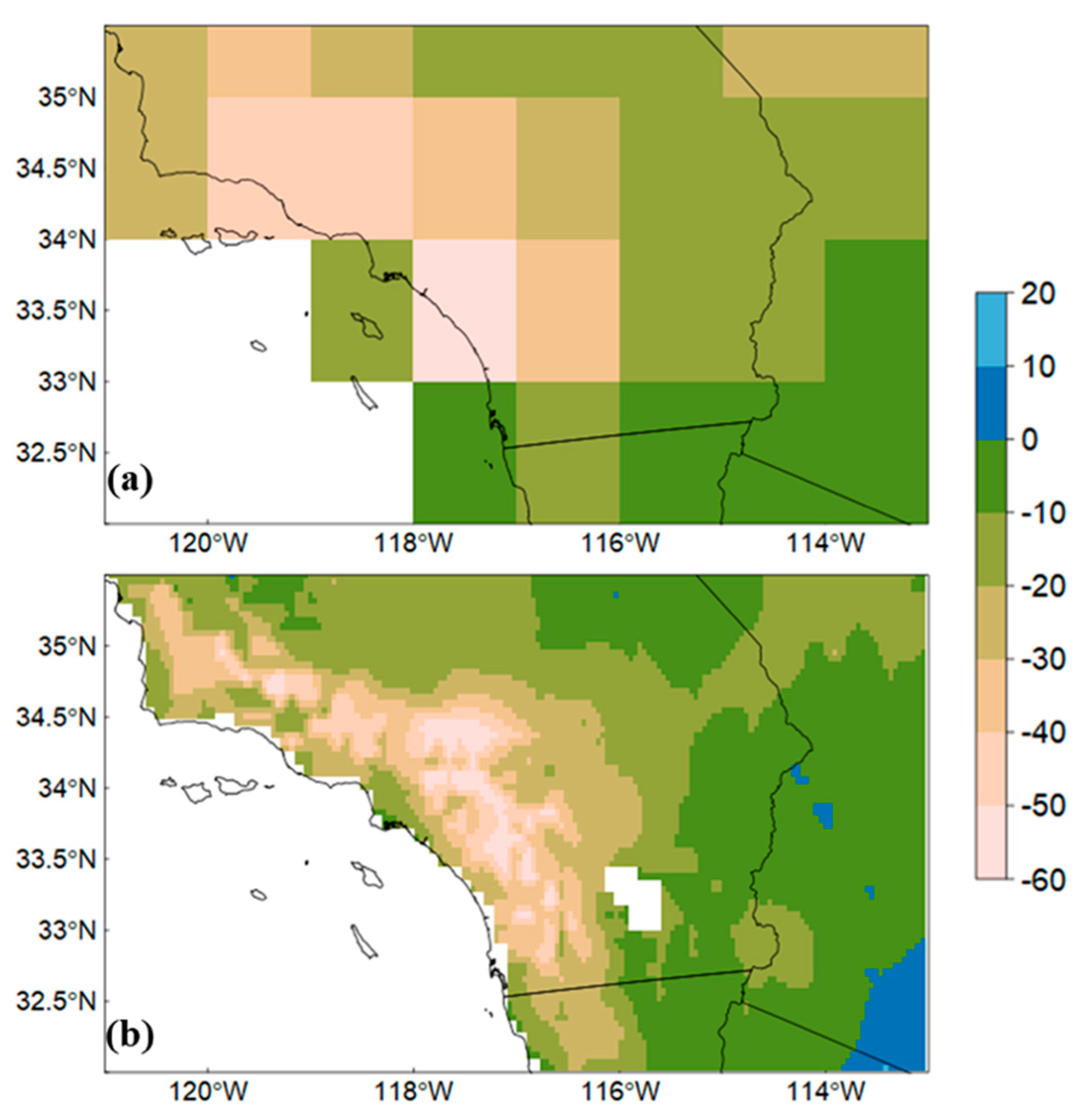
The spatial distribution of 10-year average TWS anomalies is shown in Figure 5a,b. GRACE estimates showed declining TWS throughout the entire study area. The strongest declines were found along the coastal areas between 33° N and 35° N, where values below −30 mm could be observed. The largest drying was located between Los Angeles and San Diego (Figure 1a), where TWS dropped by −55 mm over the 10 years.
In general, the new SSIB-SIMGM model was able to simulate the main features of the TWS anomalies distribution, with the lowest values located along the coastal areas and highest along the border with Mexico (Figure 5b). Due to its higher spatial resolution, the model was able to significantly enhance the heterogeneity of the TWS anomaly distribution. TWS anomalies in the coastal areas are particularly difficult to assess through GRACE’s coarse-resolution data due to the influence of the nearby ocean [36]. The 10-year domain-average TWS anomaly for GRACE and SSIB-SIMGM was −23.3 mm and −21.0 mm, respectively. In general, the partially-coupled model was able to simulate the temporal evolution and spatial distribution of TWS anomalies in Southern California.
3.2. WRF-SSIB-SIMGM Model
Unlike the partially-coupled model, the forcing data for the surface and aquifer models described in this section were simulated by the WRF model. Initial soil conditions and aquifer water storage for the simulations were the same as those used for the partially-coupled model, as were the domain size and resolution, land cover, and topographic distributions.
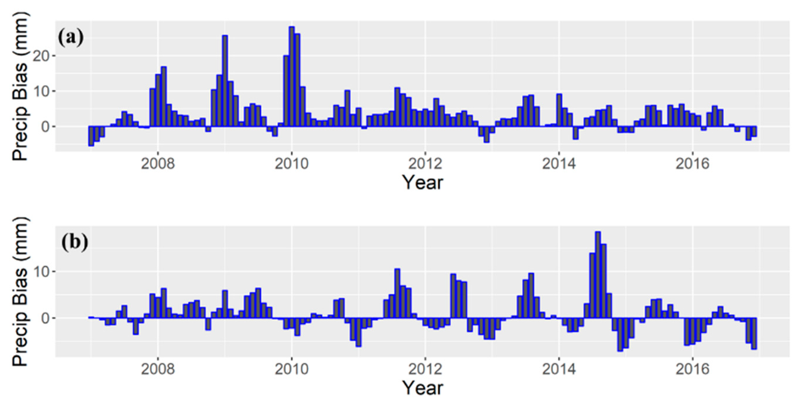
In general, results from the fully and partially coupled models were similar over the Coastal Basin aquifers (Figure 3a). The fully-coupled model overestimated the precipitation over that aquifer, between 2008 and 2010 (Figure 6a), which resulted in an overestimation of TWS recharge when compared to the partially-coupled model results and GRACE estimates. For the remaining years, the modeled precipitation biases were smaller and TWS results were consistent with the partially-coupled model results. On average, the TWS anomaly’s RMSE and temporal correlation compared to GRACE were respectively 34.7 mm month−1 and 0.87 (Table 2).
The fully-coupled model also overestimated precipitation over the Basin and Range aquifer region, especially during the last three years of simulation (Figure 6b). The modeled average precipitation for those years was approximately twice as much as observations. The excessive precipitation produced by WRF-SSIB-SIMGM caused a positive bias in TWS anomaly compared to GRACE (Figure 4a). On average, TWS anomaly RMSE and temporal correlation compared to GRACE was 18.1 mm month−1 and 0.91 respectively (Table 2). Furthermore, similarly to the results obtained with the partially-coupled model, time lag between the fully-coupled model’s precipitation and TWS anomaly maxima were one month shorter than those observed from GRACE TWS estimates.
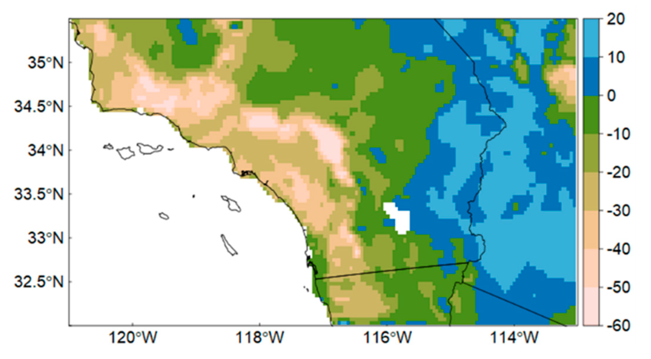
In general, the fully-coupled model generated a weaker 10-year mean anomaly distribution than the partially-coupled model due to the wet bias in simulated rainfall (Figure 7). Along the coast, only a small area showed 10-year average anomalies below −120 mm month−1, whereas both GRACE and the partially-coupled model showed a much more extensive area. Over the Basin and Range aquifer system, the fully-coupled model showed positive TWS anomalies, which were not consistent with either the GRACE estimates or the partially-coupled model results.
4. Discussion
The results presented show that the partially-coupled model formed by the SSIB land surface and SIMGM aquifer models was able to simulate the temporal and spatial variability of TWS anomalies in the study area. It provides a more detailed spatial representation of TWS anomalies when compared to GRACE data due to its higher spatial resolution. However, the results from the fully-coupled model clearly indicate that accurate precipitation information is essential to achieve accurate TWS simulations. Precipitation biases in the WRF-SSIB-SIMGM model during the last five years of simulation noticeably affected the quality of TWS anomaly results. Moreover, both models have a shorter precipitation-TWS lagged response time (1 month) than that observed with GRACE (2 months). Nevertheless, the two models have the potential to be useful tools for the study of surface water budget in areas that lack extensive observational networks.
Since the partially-coupled model can reproduce the annual evolution of TWS well in both aquifers, it would be interesting to further examine the relationship between TWS anomaly and the two other components of surface water budget: runoff and evapotranspiration during a water year. A water year is defined as the time between October and September of the following year. Over both aquifers, evapotranspiration loss is the predominant component of the water budget (Figure 8a,b). Changes in evapotranspiration, TWS, and runoff account for approximately 65%, 24% and 11% of monthly precipitation on average for the Coastal Basin aquifer. For the Basin Range system those rates are 72%, 20%, and 8%, respectively. The skewed distribution of available water towards evapotranspiration reflects the semi-arid climate of these areas, which are characterized by long dry summers.
It is also interesting to note that the partitioning of precipitation into the three water budget components varies from year to year. For example, in the 2010 water year in the Costal Basin aquifer, runoff and TWS together accounted for as much of the precipitation as evapotranspiration. However, in 2012, runoff and TWS added to about 10% of total evapotranspiration for that year. We believe that this variability could be associated with the type of precipitation event (long light versus short heavy), which impacts runoff and infiltration rates, as well as with the vegetation state (green versus brown) in the area, which affects photosynthesis and evapotranspiration rates.
Finally, we examined the partitioning of the TWS anomaly into soil moisture and aquifer water anomalies (Figure 8c,d). In general, soil moisture anomalies displayed a higher variability than groundwater. The results showed that average groundwater recharge occurred only in 2010 and 2011 for both aquifers, with the 2011 water year being the more significant recharging event. Groundwater discharge was more intense in 2013 and 2014 over the Coastal Basin, and for 2015 and 2016 over the Basin and Range aquifer system. In general, the soil moisture anomaly accounts for nearly 65% and 75% of the total TWS anomaly observed between 2007 and 2016.
5. Conclusions
We introduced two versions of a new atmosphere-land-aquifer modeling system and described the performance of simulated TWS anomalies in Southern California during a 10-year period marked by drought conditions. In the first version, the aquifer (SIMGM) and the land surface (SSIB) models were coupled and driven by the reanalysis data. Results indicated that this partially-coupled model was capable of simulating the TWS anomalies in the two main aquifer systems located in the study area. The model’s TWS anomaly RMSE and temporal correlation calculated against GRACE estimates were 28.6 mm month−1 and 0.90 (P < 0.001) for the Coastal Basin aquifer system, and 14.3 mm month−1 and 0.94 (P < 0.001) for the Basin and Range aquifer system. In general, this model simulated the temporal variability of TWS anomaly well, but underestimated the decline in TWS towards the end of the period when the drought was more intense.
A fully-coupled version of the model formed by the addition of the WRF atmospheric model was also evaluated. In general, results from this model were less accurate. Comparison against GRACE data yields higher RMSE for both aquifer systems. On the other hand, temporal correlations for the TWS anomaly are similar to the partially-coupled model. The main cause of the lower accuracy in the fully-coupled model’s results were the poor precipitation simulations, especially in the eastern portion of the study area, which degraded TWS results. This study suggests that accurate seasonal TWS anomaly forecasts may be difficult to achieve as meteorological models struggle to produce accurate regional precipitation forecasts.
The relationship between TWS, runoff, and evapotranspiration during the drought years was also examined based on the offline model results. On average, the total precipitation shortage during the drought years resulted in a TWS, evapotranspiration, and runoff decline of approximately 24%, 65%, and 11% for the Coastal Basin aquifer system, and 20%, 72%, and 8% for the Basin and Range system, respectively. In general, changes in the amount of soil moisture accounted for about 65% and 75% of the total TWS anomaly observed between 2007 and 2016 over the aquifer systems.
It should be noted that the baseflow decay factors used in these simulations were obtained through a simple calibration against water table measurements. We expect that a more advanced method for the estimation of this parameter could improve the results. Despite the biases, the results indicate that the newly coupled models could be an important tool to further our understanding of the role land cover and precipitation play in determining terrestrial water storage availability at regional and local scales.
Supplementary Materials
The following are available online at https://www.mdpi.com/2073-4441/12/3/808/s1, Table S1: List of USGS wells used for the calibration of the baseflow decay factor (F). Water table depth data was downloaded from https://waterdata.usgs.gov/usa/nwis/gw.
Author Contributions
Conceptualization, methodology, and validation, F.D.S. and D.E.R.; writing—original draft preparation, F.D.S.; visualization, F.D.S.; project administration, F.D.S.; funding acquisition, F.D.S. All authors have read and agreed to the published version of the manuscript.
Funding
This research was funded by the San Diego State University Grants Program (grant number 242527) and was supported by the Center for Earth Systems Analysis Research at the San Diego State University Department of Geography.
Acknowledgments
The authors thank University of Arizona Guo-Yue Niu for his help and expertise and the National Center for Atmospheric Research for providing the forcing data for the model simulations.
Conflicts of Interest
The authors declare no conflicts of interest. The funders had no role in the design of the study; in the collection, analyses, or interpretation of data; in the writing of the manuscript, or in the decision to publish the results.
References
- Thomas, A.C.; Reager, J.T.; Famiglietti, J.S.; Rodell, M. A GRACE-based water storage deficit approach for hydrological drought characterization. Geophys. Res. Lett. 2014, 41, 1537–1545. [Google Scholar] [CrossRef] [Green Version]
- Voss, K.A.; Famiglietti, J.S.; Lo, M.; de Linage, C.; Rodell, M.; Swenson, S.C. Groundwater depletion in the Middle East from GRACE with implications for transboundary water management in the Tigris-Euphrates-Western Iran region. Water Resour. Res. 2013, 49, 904–914. [Google Scholar] [CrossRef] [PubMed] [Green Version]
- Long, D.; Scanlon, B.R.; Longuevergne, L.; Sun, A.Y.; Fernando, D.N.; Save, H. GRACE satellite monitoring of large depletion in water storage in response to the 2011 drought in Texas. Geophys. Res. Lett. 2013, 40, 3395–3401. [Google Scholar] [CrossRef] [Green Version]
- Census 2010 News | U.S. Census Bureau Announces 2010 Census Population Counts—Apportionment Counts Delivered to President. Available online: https://web.archive.org/web/20101224044247/http://2010.census.gov/news/releases/operations/cb10-cn93.html (accessed on 9 February 2020).
- De Sales, F.; Xue, Y. Dynamic downscaling of 22-year CFS winter seasonal hindcasts with the UCLA-ETA regional climate model over the United States. Clim. Dyn. 2013, 41, 255–275. [Google Scholar] [CrossRef]
- Ustin, S.L.; Roberts, D.A.; Pinzón, J.; Jacquemoud, S.; Gardner, M.; Scheer, G.; Castañeda, C.M.; Palacios-Orueta, A. Estimating Canopy Water Content of Chaparral Shrubs Using Optical Methods. Remote Sens. Environ. 1998, 65, 280–291. [Google Scholar] [CrossRef]
- Alley, W.M.; Healy, R.W.; LaBaugh, J.W.; Reilly, T.E. Flow and Storage in Groundwater Systems. Science 2002, 296, 1985–1990. [Google Scholar] [CrossRef] [PubMed] [Green Version]
- California’s Groundwater Update 2013: A Compilation of Enhanced Content for California Water Plan Update 2013. California Water Library. Available online: https://water.ca.gov/LegacyFiles/waterplan/docs/groundwater/update2013/other/webex_presentations/july_27_2015/2-3_California_Groundwater_Update_2013_SR_SC_SFB_HRs_Final.pdf (accessed on 1 December 2019).
- IPCC. Climate Change 2014: Synthesis Report. Contribution of Working Groups I, II and III to the Fifth Assessment Report of the Intergovernmental Panel on Climate Change; Core Writing Team, Pachauri, R.K., Meyer, L.A., Eds.; IPCC: Geneva, Switzerland, 2014; p. 151. [Google Scholar]
- Famiglietti, J.S.; Lo, M.; Ho, S.L.; Bethune, J.; Anderson, K.J.; Syed, T.H.; Swenson, S.C.; de Linage, C.R.; Rodell, M. Satellites measure recent rates of groundwater depletion in California’s Central Valley. Geophys. Res. Lett. 2011, 38. [Google Scholar] [CrossRef] [Green Version]
- Krueger, E.S.; Ochsner, T.E.; Engle, D.M.; Carlson, J.D.; Twidwell, D.; Fuhlendorf, S.D. Soil Moisture Affects Growing-Season Wildfire Size in the Southern Great Plains. Soil Sci. Soc. Am. J. 2015, 79, 1567–1576. [Google Scholar] [CrossRef]
- Jensen, D.; Reager, J.T.; Zajic, B.; Rousseau, N.; Rodell, M.; Hinkley, E. The sensitivity of US wildfire occurrence to pre-season soil moisture conditions across ecosystems. Environ. Res. Lett. 2018, 13, 014021. [Google Scholar] [CrossRef]
- Tian, S.; Tregoning, P.; Renzullo, L.J.; van Dijk, A.I.J.M.; Walker, J.P.; Pauwels, V.R.N.; Allgeyer, S. Improved water balance component estimates through joint assimilation of GRACE water storage and SMOS soil moisture retrievals. Water Resour. Res. 2017, 53, 1820–1840. [Google Scholar] [CrossRef]
- Niu, G.-Y.; Yang, Z.-L.; Dickinson, R.E.; Gulden, L.E. A simple TOPMODEL-based runoff parameterization (SIMTOP) for use in global climate models. J. Geophys. Res. Atmos. 2005, 110. [Google Scholar] [CrossRef] [Green Version]
- Niu, G.Y.; Yang, Z.L.; Dickinson, R.E.; Gulden, L.E.; Su, H. Development of a simple groundwater model for use in climate models and evaluation with Gravity Recovery and Climate Experiment data. J. Geophys. Res. Atmos. 2007, 112. [Google Scholar] [CrossRef]
- Jiang, X.; Niu, G.-Y.; Yang, Z.-L. Impacts of vegetation and groundwater dynamics on warm season precipitation over the Central United States. J. Geophys. Res. Atmos. 2009, 114. [Google Scholar] [CrossRef]
- Niu, G.-Y.; Yang, Z.-L.; Mitchell, K.E.; Chen, F.; Ek, M.B.; Barlage, M.; Kumar, A.; Manning, K.; Niyogi, D.; Rosero, E.; et al. The community Noah land surface model with multiparameterization options (Noah-MP): 1. Model description and evaluation with local-scale measurements. J. Geophys. Res. Atmos. 2011, 116. [Google Scholar] [CrossRef] [Green Version]
- Cai, X.; Yang, Z.-L.; David, C.H.; Niu, G.-Y.; Rodell, M. Hydrological evaluation of the Noah-MP land surface model for the Mississippi River Basin. J. Geophys. Res. Atmos. 2014, 119, 23–38. [Google Scholar] [CrossRef]
- Swenson, S.C.; Lawrence, D.M. A GRACE-based assessment of interannual groundwater dynamics in the Community Land Model. Water Resour. Res. 2015, 51, 8817–8833. [Google Scholar] [CrossRef]
- Stampoulis, D.; Reager, J.T.; David, C.H.; Andreadis, K.M.; Famiglietti, J.S.; Farr, T.G.; Trangsrud, A.R.; Basilio, R.R.; Sabo, J.L.; Osterman, G.B.; et al. Model-data fusion of hydrologic simulations and GRACE terrestrial water storage observations to estimate changes in water table depth. Adv. Water Resour. 2019, 128, 13–27. [Google Scholar] [CrossRef]
- Wagner, S.; Fersch, B.; Yuan, F.; Yu, Z.; Kunstmann, H. Fully coupled atmospheric-hydrological modeling at regional and long-term scales: Development, application, and analysis of WRF-HMS. Water Resour. Res. 2016, 52, 3187–3211. [Google Scholar] [CrossRef] [Green Version]
- Skamarock, C.; Klemp, B.; Dudhia, J.; Gill, O.; Barker, D.; Duda, G.; Huang, X.; Wang, W.; Powers, G. A Description of the Advanced Research WRF Version 3; University Corporation for Atmospheric Research: Boulder, CO, USA, 2008. [Google Scholar]
- Xue, Y.; Sellers, P.J.; Kinter, J.L.; Shukla, J. A simplified biosphere model for global climate studies. J. Clim. 1991, 4, 345–364. [Google Scholar] [CrossRef] [Green Version]
- Griffin, D.; Anchukaitis, K.J. How unusual is the 2012–2014 California drought? Geophys. Res. Lett. 2014, 41, 9017–9023. [Google Scholar] [CrossRef] [Green Version]
- Dong, C.; MacDonald, G.M.; Willis, K.; Gillespie, T.W.; Okin, G.S.; Williams, A.P. Vegetation Responses to 2012–2016 Drought in Northern and Southern California. Geophys. Res. Lett. 2019, 46, 3810–3821. [Google Scholar] [CrossRef]
- De Sales, F.; Xue, Y.K.; Okin, G.S. Impact of burned areas on the northern African seasonal climate from the perspective of regional modeling. Clim. Dyn. 2016, 47, 3393–3413. [Google Scholar] [CrossRef] [Green Version]
- Xue, Y.K.; Fennessy, M.J.; Sellers, P.J. Impact of vegetation properties on US summer weather prediction. J. Geophys. Res. Atmos. 1996, 101, 7419–7430. [Google Scholar] [CrossRef] [Green Version]
- Clapp, R.B.; Hornberger, G.M. Empirical equations for some soil hydraulic properties. Water Resour. Res. 1978, 14, 601–604. [Google Scholar] [CrossRef] [Green Version]
- Mesinger, F.; DiMego, G.; Kalnay, E.; Mitchell, K.; Shafran, P.C.; Ebisuzaki, W.; Jović, D.; Woollen, J.; Rogers, E.; Berbery, E.H.; et al. North American Regional Reanalysis. Bull. Am. Meteorol. Soc. 2006, 87, 343–360. [Google Scholar] [CrossRef] [Green Version]
- Ferrier, B. A double-moment multiple-phase 4-class bulk ice scheme 1. description. J. Atmos. Sci. 1994, 51, 249–280. [Google Scholar] [CrossRef] [Green Version]
- Gu, Y.; Liou, K.N.; Ou, S.C.; Fovell, R. Cirrus cloud simulations using WRF with improved radiation parameterization and increased vertical resolution. J. Geophys. Res. Atmos. 2011, 116. [Google Scholar] [CrossRef]
- Hong, S.Y.; Noh, Y.; Dudhia, J. A new vertical diffusion package with an explicit treatment of entrainment processes. Mon. Weather Rev. 2006, 134, 2318–2341. [Google Scholar] [CrossRef] [Green Version]
- Grell, G.A.; Devenyi, D. A generalized approach to parameterizing convection combining ensemble and data assimilation techniques. Geophys. Res. Lett. 2002, 29. [Google Scholar] [CrossRef] [Green Version]
- Famiglietti, J.S.; Rodell, M. Water in the Balance. Science 2013, 340, 1300–1301. [Google Scholar] [CrossRef]
- Swenson, S.C. GRACE Monthly Land Water Mass Grids NETCDF RELEASE 5.0. Ver. 5.0; PO.DAAC: Pasadena, CA, USA, 2012. [Google Scholar] [CrossRef]
- Landerer, F.W.; Swenson, S.C. Accuracy of scaled GRACE terrestrial water storage estimates. Water Resour. Res. 2012, 48. [Google Scholar] [CrossRef]
- Dahle, C.; Murböck, M.; Flechtner, F.; Dobslaw, H.; Michalak, G.; Neumayer, K.H.; Abrykosov, O.; Reinhold, A.; König, R.; Sulzbach, R.; et al. The GFZ GRACE RL06 Monthly Gravity Field Time Series: Processing Details and Quality Assessment. Remote Sens. 2019, 11, 2116. [Google Scholar] [CrossRef] [Green Version]
- Watkins, M.M.; Wiese, D.N.; Yuan, D.-N.; Boening, C.; Landerer, F.W. Improved methods for observing Earth’s time variable mass distribution with GRACE using spherical cap mascons. J. Geophys. Res. Solid Earth 2015, 120, 2648–2671. [Google Scholar] [CrossRef]
- Chen, J.L.; Wilson, C.R.; Tapley, B.D.; Yang, Z.L.; Niu, G.Y. 2005 drought event in the Amazon River basin as measured by GRACE and estimated by climate models. J. Geophys. Res. Solid Earth 2009, 114. [Google Scholar] [CrossRef]
- Ground Water Atlas of the United States: Introduction and National Summary. Available online: https://pubs.er.usgs.gov/publication/ha730A (accessed on 28 December 2019).
- Zhang, Y.; He, B.; Guo, L.; Liu, D. Differences in Response of Terrestrial Water Storage Components to Precipitation over 168 Global River Basins. J. Hydrometeorol. 2019, 20, 1981–1999. [Google Scholar] [CrossRef]
- Zhang, Y.; He, B.; Guo, L.; Liu, J.; Xie, X. The relative contributions of precipitation, evapotranspiration, and runoff to terrestrial water storage changes across 168 river basins. J. Hydrol. 2019, 579, 124194. [Google Scholar] [CrossRef]
Figure 1.
(a) Topographic map of Southern California and the domain used for the model simulations (dashed lines). (b) The two principal aquifer systems located within the model domain: the coastal basin aquifer system and the basin and range aquifer system. The major metropolitan areas in the domain are also shown in (a): Los Angeles, Riverside, San Diego, and Las Vegas.

Figure 2.
Average United States Geological Survey (USGS) well and simulated water table depth anomalies in the (a) Coastal Basin and (b) Basin and Range aquifer systems between October 2008 and March 2011 for baseflow decay factors (F) ranging from 1.5 to 8 m−1. Anomalies were calculated based on 2008–2011 average baseline. Well locations are listed in Table S1.

Figure 3.
(a) GRACE, SSIB-SIMGM, and WRF-SSIB-SIMGM monthly TWS anomalies based on the 2007–2010 baseline and (b) monthly precipitation for the Coastal Basin aquifer system between 2007 and 2016. Dashed line in (b) represents an average precipitation annual cycle over the aquifer.
Figure 3.
(a) GRACE, SSIB-SIMGM, and WRF-SSIB-SIMGM monthly TWS anomalies based on the 2007–2010 baseline and (b) monthly precipitation for the Coastal Basin aquifer system between 2007 and 2016. Dashed line in (b) represents an average precipitation annual cycle over the aquifer.

Figure 4.
(a) GRACE, SSIB-SIMGM, and WRF-SSIB-SIMGM monthly TWS anomalies based on the 2007–2010 baseline and (b) monthly precipitation for the Coastal Basin aquifer system between 2007 and 2016. Dashed line in (b) represents an average precipitation annual cycle over the aquifer.
Figure 4.
(a) GRACE, SSIB-SIMGM, and WRF-SSIB-SIMGM monthly TWS anomalies based on the 2007–2010 baseline and (b) monthly precipitation for the Coastal Basin aquifer system between 2007 and 2016. Dashed line in (b) represents an average precipitation annual cycle over the aquifer.

Figure 5.
2007–2016 average monthly TWS anomaly for (a) GRACE and (b) SSIB-SIMGM. Anomalies calculated based on the 2007–2010 average baseline. Unit: mm.
Figure 5.
2007–2016 average monthly TWS anomaly for (a) GRACE and (b) SSIB-SIMGM. Anomalies calculated based on the 2007–2010 average baseline. Unit: mm.

Figure 6.
WRF-SSIB-SIMGM monthly precipitation bias for (a) the Coastal Basin aquifer and (b) the Basin and Range aquifer systems compared to North American Regional Reanalysis (NARR) data.
Figure 6.
WRF-SSIB-SIMGM monthly precipitation bias for (a) the Coastal Basin aquifer and (b) the Basin and Range aquifer systems compared to North American Regional Reanalysis (NARR) data.

Figure 7.
2007–2016 monthly average TWS anomaly simulated by the fully-coupled model. Anomalies calculated based on the 2007–2010 average baseline. Unit: mm.
Figure 7.
2007–2016 monthly average TWS anomaly simulated by the fully-coupled model. Anomalies calculated based on the 2007–2010 average baseline. Unit: mm.

Figure 8.
Water-year evapotranspiration, terrestrial water storage, and runoff rates for (a) Coastal Basin and (b) Basin and Range aquifer systems; and aquifer (WT) and soil moisture (SM) storages for (c) Coastal Basin and (d) Basin and Range aquifer systems. Unit: mm month−1.
Figure 8.
Water-year evapotranspiration, terrestrial water storage, and runoff rates for (a) Coastal Basin and (b) Basin and Range aquifer systems; and aquifer (WT) and soil moisture (SM) storages for (c) Coastal Basin and (d) Basin and Range aquifer systems. Unit: mm month−1.


Table 1.
Impact of baseflow decay factor (m−1) on the SSIB-SIMGM simulations for the two main aquifer systems in the study area. Statistics represent 4-year domain-average terrestrial water storage (TWS) anomaly bias (mm), root-mean squared error (RMSE) (mm), and temporal correlation (TCOR). * and ** indicates correlation significance at 90% and 99% confidence levels, respectively.
| Metric | F = 8 | F = 6 | F = 4 | F = 3 | F = 2 | F = 1.5 |
|---|---|---|---|---|---|---|
| Basin and Range Aquifers | ||||||
| Bias | 16.5 | 16.1 | 14.7 | 9.8 | −3.4 | −16.9 |
| RMSE | 20.9 | 20.3 | 18.6 | 12.7 | 4.6 | 18.3 |
| TCOR | −0.82 | −0.81 | −0.75 | −0.24 | 0.90 ** | 0.97 ** |
| Coastal Basin Aquifers | ||||||
| Bias | 26.2 | 25.3 | 22.3 | 14.0 | −4.0 | −20.4 |
| RMSE | 33.8 | 32.5 | 28.7 | 19.7 | 9.5 | 22.7 |
| TCOR | 0.10 | 0.03 | 0.12 | 0.39 * | 0.78 ** | 0.78 ** |
Table 2.
SSIB-SIMGM and WRF-SSIB-SIMGM performances for the Coastal and Basin and Range aquifer systems. Includes the average bias, root-mean-squared error (RMSE) (mm/month), and temporal correlation (TCOR). All correlation coefficients are significant at a 99% confidence interval.
Table 2.
SSIB-SIMGM and WRF-SSIB-SIMGM performances for the Coastal and Basin and Range aquifer systems. Includes the average bias, root-mean-squared error (RMSE) (mm/month), and temporal correlation (TCOR). All correlation coefficients are significant at a 99% confidence interval.
| Aquifers | Data | Mean | Bias | RMSE | TCOR |
|---|---|---|---|---|---|
| Coastal Basin | GRACE | −47.7 | - | - | - |
| SSIB-SIMGM | −44.6 | 3.8 | 28.6 | 0.90 | |
| WRF-SSIB-SIMGM | −49.4 | −1.7 | 34.7 | 0.87 | |
| Basin and Range | GRACE | −25.5 | - | - | - |
| SSIB-SIMGM | −19.6 | 6.3 | 14.3 | 0.94 | |
| WRF-SSIB-SIMGM | −12.3 | 9.1 | 18.1 | 0.91 |
© 2020 by the authors. Licensee MDPI, Basel, Switzerland. This article is an open access article distributed under the terms and conditions of the Creative Commons Attribution (CC BY) license (http://creativecommons.org/licenses/by/4.0/).
Share and Cite
MDPI and ACS Style
De Sales, F.; Rother, D.E. A New Coupled Modeling Approach to Simulate Terrestrial Water Storage in Southern California. Water 2020, 12, 808. https://doi.org/10.3390/w12030808
AMA Style
De Sales F, Rother DE. A New Coupled Modeling Approach to Simulate Terrestrial Water Storage in Southern California. Water. 2020; 12(3):808. https://doi.org/10.3390/w12030808
Chicago/Turabian StyleDe Sales, Fernando, and David E. Rother. 2020. "A New Coupled Modeling Approach to Simulate Terrestrial Water Storage in Southern California" Water 12, no. 3: 808. https://doi.org/10.3390/w12030808
Note that from the first issue of 2016, this journal uses article numbers instead of page numbers. See further details here.