Poroacoustic Traveling Waves under the Rubin–Rosenau–Gottlieb Theory of Generalized Continua

Abstract

We investigate linear and nonlinear poroacoustic waveforms under the Rubin–Rosenau– Gottlieb (RRG) theory of generalized continua. Working in the context of the Cauchy problem, on both the real line and the case with periodic boundary conditions, exact and asymptotic expressions are obtained. Numerical simulations are also presented, von Neumann–Richtmyer “artificial” viscosity is used to derive an exact kink-type solution to the poroacoustic piston problem, and possible experimental tests of our findings are noted. The presentation concludes with a discussion of possible follow-on investigations.

1. Introduction

What is known today as the “RRG theory” was put forth by Rubin et al. [1] in 1995. This phenomenological-based theory of generalized continua is thought capable of modeling dispersive effects caused by the introduction of a medium’s characteristic length, which Rubin et al. denote as $\alpha$. Under RRG theory, $\alpha$ is regarded as an inherent material property. From the modeling standpoint, this theory exhibits a number of appealing features, the two most important of which are the following: (i) it is only the pressure stress (i.e., isotropic) part of the Cauchy (i.e., total) stress tensor and the specific Helmholtz free energy that are modified, but these modifications are achieved by adding perburtative terms, which must satisfy certain constraint equations, to the constitutive relations of the former and latter; and (ii), no additional boundary nor initial conditions, beyond those required to solve classically formulated problems, are needed ([1], p. 4063).

To date, RRG theory has only been applied to single-phase media; see, e.g., Ref. [2] and those cited therein. Hence, there is an obvious need to investigate the nature of the solutions, e.g., those of the traveling wave type, predicted by this theory in the case of multi-phase media.

Accordingly, the aim of this communication is to carry out a preliminary investigation of RRG theory in the context of acoustic problems involving propagation in dual-phase (specifically, fluid + solid) media—dual-phase media being, of course, the simplest case of multi-phase media. Employing both analytical and numerical methodologies, we consider linear and finite-amplitude poroacoustic propagation under the RRG-based generalization of what some refer to as the Brinkman poroacoustic model (BPM) (Although he does not refer to it as such, the general, multi-D, version of the BPM follows on setting $C=0$ in Burmeister [3].). Here, it should be noted that the original version of the drag law on which the BPM is based reads (see, e.g., Refs. [4,5])

$$\nabla P=\tilde{\mu }\chi {\nabla }^2\mathbf{u}-(\mu \chi /K)\mathbf{u}.$$

(1)

In this relation, $\mathbf{u}$ is the intrinsic average velocity of the fluid, which it is related to $\mathbf{v}$, the Darcy velocity, via the Dupuit–Forchheimer relationship $\mathbf{v}=\chi \mathbf{u}$ ([4], p. 5); P is a pressure, an intrinsic quantity, which is not the thermodynamic pressure ([4], §1.4.1); $\mu$ is the usual shear viscosity coefficient; $\tilde{\mu }$ is an effective viscosity ([4], §1.5.3), which is often referred to as the Brinkman viscosity; and $K>0$ and $\chi \in (0,1)$, the permeability and porosity of the solid matrix, are assumed to be constants. We should also note that Equation (1) reduces to Darcy’s law on setting $\tilde{\mu }:=0$.

Before beginning our analysis, we should point out that when traveling wave solutions (TWS)s in the form of kinks are encountered below, their shock thicknesses shall be expressed using Prandtl’s definition (see, e.g., (Ref. [6], p. 680)), viz.:

$$\mathrm{shock} \mathrm{thickness}:=\frac{\mathfrak{F}(-\infty )-\mathfrak{F}(+\infty )}{{\displaystyle \underset{\mathfrak{z}\in \mathbb{R}}{max}}|\mathrm{d}\mathfrak{F}\left(\mathfrak{z}\right)/\mathrm{d}\mathfrak{z}|},$$

(2)

where $\mathfrak{z}$ represents the wave (i.e., similarity) variable. Herein, all traveling wave profiles shall be taken to be propagating to the right along the axis corresponding to the wave variable under consideration.

2. Mathematical Formulations

2.1. Poroacoustic Model Systems

When entropy production in the fluid, which we hereafter take to be a perfect gas [7], is ignored (i.e., we take the flow to be homentropic ([7], p. 60)) and the porous matrix is regarded as being both stationary and composed of a thermally non-conducting rigid solid, the 1D versions of the RRG-based model we propose and the BPM become, in the case of propagation along the x-axis,

$${\varrho }_t+u{\varrho }_x+\varrho u_x=0,$$

(3a)

$$\varrho (u_t+u{u}_x)=\tilde{\mu }\chi u_{xx}-(\mu \chi /K)u-\left\{\begin{array}{cc}{\mathcal{P}}_x,\hfill & \mathrm{BPM},\hfill \\ [\mathcal{P}-2{\alpha }^2\varrho (u_{xt}+u{u}_{xx}){]}_x,\hfill & \mathrm{RRG},\hfill \end{array}\right.$$

(3b)

$$\mathcal{P}\approx {\mathcal{P}}_0{(\varrho /{\varrho }_0)}^{\gamma }\hspace{1em}(\mathfrak{n}\approx {\mathfrak{n}}_0).$$

(3c)

In System (3), $\mathcal{P}(>0)$ is the thermodynamic pressure; $\varrho (>0)$ is the mass density of the gas; $\mathfrak{n}$ is the specific entropy of the gas; the parameter $\gamma$ denotes the ratio of specific heats, where $\gamma \in (1,5/3]$ in the case of perfect gases; we take $\alpha (>0)$, which carries the unit of length, to be a constant (That is, we have assumed the simplest version of RRG theory; see (Ref. [1], Equation (20)).); the problem geometry dictates that, here and henceforth, $\mathbf{u}=\left(u\right(x,t),0,0)$, $\mathcal{P}=\mathcal{P}(x,t)$, and $\varrho =\varrho (x,t)$; and a zero (“0”) subscript attached to a dependent variable denotes the (constant) equilibrium state value of that variable, where we note that ${\mathbf{u}}_0=(0,0,0)$.

Here, we observe that since the flow has been assumed homentropic, our RRG-based poroacoustic model is obtained by perturbing only the pressure tensor term in the BPM. Also, we record for later reference that $c_0=\sqrt{\gamma {\mathcal{P}}_0/{\varrho }_0}$ is the (constant) equilibrium state value of the sound speed, i.e., the speed of sound in the undisturbed gas; see, e.g., (Ref. [7], §4.3).

2.2. Finite-Amplitude Equation of Motion: The Case $\mu :=$ const.

We begin this sub-section with the following observation: Because $\nabla \times \mathbf{u}=(0,0,0)$ holds identically under the present (1D) geometry, it follows that $\mathbf{u}=\nabla \varphi$; therefore, $u(x,t)={\varphi }_x(x,t)$, where ${\varphi }_x$ denotes the scalar velocity potential.

Hence, on invoking the finite-amplitude approximation, and introducing the following dimensionless variables:

$$u^{\diamond }=u/U_{\mathrm{p}},\hspace{1em}s=(\varrho -{\varrho }_0)/{\varrho }_0,\hspace{1em}{\varphi }^{\diamond }=\varphi /\left(U_{\mathrm{p}}L\right),\hspace{1em}{x}^{\diamond }=x/L,\hspace{1em}{t}^{\diamond }=t(c_0/L),$$

(4)

where the positive constants L and $U_{\mathrm{p}}$ respectively denote a macro-length scale characteristic of the propagation domain and the magnitude of the peak particle velocity in the gas, it is not difficult to establish (See, e.g., the derivation performed in (Ref. [8], §2), and note that (Ref. [8], Equation (10)) is the $\sigma ,\delta :=0$ special case of Equation (5) herein.) that the $\mu :=$ const. case of System (3) reduces to the weakly-nonlinear, bi-directional, equation of motion (EoM)

$${\varphi }_{tt}-[1-2ϵ(\beta -1){\varphi }_t]{\varphi }_{xx}+ϵ{\partial }_t{\left({\varphi }_x\right)}^2=\sigma {\varphi }_{txx}+a_0^2{\varphi }_{ttxx}-\delta {\varphi }_t,$$

(5)

where here and henceforth all diamond ${(}^{\diamond })$ superscripts have been suppressed for convenience. In Equation (5), which we note reduces to the corresponding EoM for the (1D) BPM on setting $a_0:=0$, $ϵ=U_{\mathrm{p}}/c_0$ is the Mach number, where $ϵ\ll 1$ is assumed; $\delta =\nu \chi L/\left(c_{0}K\right)$ is the dimensionless Darcy coefficient, where $\nu =\mu /{\varrho }_0$ is the kinematic viscosity of the gas; $a_0$, the dimensionless version of $\alpha$, is given by $a_0=\alpha \sqrt{2}/L$; we have set $\sigma :=\chi /R{e}_{\mathrm{B}}$, where $R{e}_{\mathrm{B}}=c_{0}L/\tilde{\nu }$ is a Reynolds number, and where $\tilde{\nu }=\tilde{\mu }/{\varrho }_0$; and $\beta (>1)$ denotes the coefficient of nonlinearity [9], which in the case of a perfect gas is given by

$$\beta =(\gamma +1)/2.$$

(6)

In deriving Equation (5) we have assumed that $\delta ,\sigma ,a_0,\left|s\right|\sim \mathcal{O}\left(ϵ\right)$ and, in accordance with the finite-amplitude approximation, only nonlinear terms $\mathcal{O}\left({ϵ}^2\right)$ have been neglected.

2.3. Right-Running Equations of Motion for the Case $\mu :=$ const.

Although derived under the finite-amplitude approximation, Equation (5) is still too complicated for treatment by analytical means. Fortunately, however, the nature of the problems to be considered below is such that we may employ the uni-directional approximation to reduce the order of Equation (5) by one and confine its nonlinearity to a single (quadratic) term. Omitting the details, we find that under, say, the right-running case of this approximation (See, e.g., Crighton’s ([10], p. 16) derivation of the acoustic version of Burgers’ equation.), which in the present setting reads ${\varphi }_x\simeq -{\varphi }_t$, our EoM becomes, after making use of the relation $u(x,t)={\varphi }_x(x,t)$ and simplifying,

$$u_t+u_x+ϵ\beta u{u}_x-\frac{1}{2}{a}_0^2{u}_{txx}+\frac{1}{2}\delta u=\frac{1}{2}\sigma u_{xx},$$

(7)

which on switching to the variables $X=x-t$ and $T=t$ is further reduced to

$$u_T+ϵ\beta u{u}_X-\frac{1}{2}{a}_0^2{u}_{TXX}+\frac{1}{2}\delta u=\frac{1}{2}\sigma u_{XX}.$$

(8)

If we once again make use of the right-running approximation, which now takes the form $u_T\simeq -u_X$, to re-express only the third order term in Equation (8), which is justified since $a_0\sim \mathcal{O}\left(ϵ\right)$ (i.e., $(a_0^2/2)u_{TXX}$ is a “small” term), then Equation (8) assumes its final form, specifically,

$$u_T+ϵ\beta u{u}_X+\frac{1}{2}{a}_0^2{u}_{XXX}+\frac{1}{2}\delta u=\frac{1}{2}\sigma u_{XX},$$

(9)

a PDE which we term the damped Burgers–KdV (dBKdV) equation.

In closing this sub-section we stress that Equations (7)–(9) apply only to right-running waveforms; i.e., to problems wherein reflection (to the left) is not possible.

3. Comparison of Linearized EoMs: The Cauchy Problem

In this section we compare the BPM with its RRG-based counterpart under the linear approximation, which at the EoM level corresponds to setting $ϵ:=0$. We do so in the context of what is perhaps the best known problem from classical PDE theory.

To this this end, we consider the linearized version of Equation (9) in the setting of the following initial value problem (IVP), i.e., in the setting of the classical Cauchy problem:

$$u_T+\frac{1}{2}{a}_0^2{u}_{XXX}+\frac{1}{2}\delta u=\frac{1}{2}\sigma u_{XX},\hspace{1em}X\in \mathbb{R},T>0,$$

(10a)

$$u(X,0)=f\left(X\right),\hspace{1em}X\in \mathbb{R}.$$

(10b)

Here, we take $f\left(X\right)$, our initial condition (IC), to be defined on the real line and such that its Fourier transform exists.

On applying the Fourier transform to both Equation (10a) and the IC, and then solving the resulting (first order) ODE, it is readily shown that

$$\widehat{u}(k,T)=\widehat{f}\left(k\right)exp\left[-\frac{1}{2}\left(\delta +\sigma k^2-\mathrm{i}{a}_0^2{k}^3\right)T\right],$$

(11)

where k is the Fourier transform parameter and a hat over a quantity denotes the Fourier transform of that quantity. In turn, applying ${\mathcal{F}}^{-1}(·)$, the inverse Fourier transform, to Equation (11) gives

$$u(X,T)=\frac{1}{2\pi }exp(-\delta T/2){\int }_{-\infty }^{\infty }\widehat{f}\left(k\right)exp\left[-\frac{1}{2}\left(\sigma k^2-\mathrm{i}{a}_0^2{k}^3\right)T\right]exp\left(\mathrm{i}kX\right)\mathrm{d}k.$$

(12)

3.1. The RRG Case: $a_0>0$

Using the convolution theorem, and letting $Ai(·)$ denote the Airy function of the first kind, the RRG (i.e., $a_0>0$) case of Equation (12) can be recast in the more explicit form

$$\begin{array}{c}\hfill u(X,T)=exp(-\delta T/2){\left(\frac{2}{3a_0^{2}T}\right)}^{1/3}\\ \hfill \times {\int }_{-\infty }^{\infty }{\mathcal{F}}^{-1}& \left[\widehat{f}\left(k\right)exp\left(-\frac{1}{2}\sigma k^2\right)\right]Ai\left[(X-\mathcal{Y}){\left(\frac{2}{3a_0^{2}T}\right)}^{1/3}\right]\mathrm{d}\mathcal{Y}\hspace{1em}(T>0).\hfill \end{array}$$

(13)

For obvious reasons, the following two special cases of $f\left(X\right)$ are of particular interest:

$$\begin{array}{c}u(X,T)=exp(-\delta T/2){\left(\frac{2}{3a_0^{2}T}\right)}^{1/3}\hfill \\ \hfill \hspace{1em}\times \left\{\begin{array}{cc}\frac{1}{\sqrt{2\pi \sigma T}}{\int }_{-\infty }^{\infty }exp\left(-\frac{1}{2\sigma }{\mathcal{Y}}^2/T\right)Ai\left[(X-\mathcal{Y}){\left(\frac{2}{3a_0^{2}T}\right)}^{1/3}\right]\mathrm{d}\mathcal{Y},\hfill & f\left(X\right)=\mathfrak{d}\left(X\right)\hfill \\ \frac{1}{\sqrt{1+b\sigma T}}{\int }_{-\infty }^{\infty }exp\left[-\frac{1}{2}b{(1+b\sigma T)}^{-1}{\mathcal{Y}}^2\right]Ai\left[(X-\mathcal{Y}){\left(\frac{2}{3a_0^{2}T}\right)}^{1/3}\right]\mathrm{d}\mathcal{Y},\hfill & f\left(X\right)={\mathrm{e}}^{-b{X}^2/2}\hfill \end{array}\right.\hspace{1em}(T>0).\end{array}$$

(14)

Here, $\mathfrak{d}(·)$ denotes the Dirac delta function and $b(>0)$ is a (dimensionless) constant.

3.2. The BPM Case: $a_0:=0$

If we assume instead the BPM, then the solution of IVP (10) is readily obtained on setting $a_0:=0$ in Equation (12); for the two aforementioned cases of $f\left(X\right)$, we find that

$$u(X,T)=\left\{\begin{array}{cc}\left[\frac{exp(-\delta T/2)}{\sqrt{2\pi \sigma T}}\right]exp\left(-\frac{1}{2\sigma }{X}^2/T\right),\hfill & f\left(X\right)=\mathfrak{d}\left(X\right)\hfill \\ \left[\frac{exp(-\delta T/2)}{\sqrt{1+b\sigma T}}\right]exp\left[-\frac{1}{2}b{(1+b\sigma T)}^{-1}{X}^2\right],\hfill & f\left(X\right)={\mathrm{e}}^{-b{X}^2/2}\hfill \end{array}\right.\hspace{1em}(T>0).$$

(15)

3.3. Remarks: RRG vs. BPM

With regard to the Gaussian IC, the primary difference between the linearized RRG and BPM cases is that the pulse profile corresponding to the former instantly becomes oscillatory about the X-axis, due to the Airy function in its integrand, while that of the latter maintains, for all $T>0$, the shape and strict positivity of the initiating Gaussian. The clearly contrasting behaviors exhibited by these two models should, therefore, allow researchers to experimentally determine which of the two best describes propagation in a given poroacoustic system.

4. Comparison of Right-Running, Weakly-Nonlinear, EoMs: Special Cases with $\mu :=$ const.

Before examining it in its most general form, and for the benefit of those readers who are not well acquainted with the intricacies of nonlinear evolution equations, it is instructive to first review selected special cases of Equation (9). The right-running models discussed in the next three sub-sections, all of which, it should be noted, have applications beyond poroacoustics, will each have a role to play in the analysis performed in Section 4.4.

4.1. Case (I): Damped KdV (dKdV) Equation

This case follows on setting $\sigma :=0$ (i.e., setting $\tilde{\mu }:=0$), under which Equation (9) reduces to

$$u_T+ϵ\beta u{u}_X+\frac{1}{2}{a}_0^2{u}_{XXX}+\frac{1}{2}\delta u=0.$$

(16)

This PDE, we observe, is the RRG-modified version of the right-running Darcy–Jordan model; see Section 4.3 below.

Since we have assumed $\delta \ll 1$, applying the Kryloff–Bogoliubov asymptotic expansion method to the dKdV equation yields, as Ott and Sudan [11] have shown, the large-T expression

$$u(X,T)\sim exp\left(-2\delta T/3\right){\mathrm{sech}}^2\left[(\zeta /a_0)\sqrt{\frac{ϵ\beta }{6}exp\left(-2\delta T/3\right)}\right],\hspace{1em}T\sim \mathcal{O}(1/\delta ),$$

(17)

where we have taken $N\left(0\right)=1$ (see Ref. [11]), and we let

$$\zeta =X-\frac{ϵ\beta }{2\delta }\left[1-exp\left(-\frac{2}{3}\delta T\right)\right];$$

(18)

see also Ref. [12], as well as Ref. [13] (Ref. [13] contains a number of recently identified typographical errors; see Appendix A below.) and those cited therein. Equation (17) represents a damped, and decelerating, solitary waveform, and as such it cannot be a soliton in the classical sense [14]. Note, however, that the acoustic version of the classic soliton solution of the KdV equation (see Ref. [8]) is recovered as the limiting case

$$u(X,T)={\mathrm{sech}}^2\left[a_0^{-1}(X-ϵ\beta T/3)\sqrt{\frac{ϵ\beta }{6}}\right]\hspace{1em}(\delta \to 0).$$

(19)

4.2. Case (II): Damped Burgers’ Equation

This case, which corresponds to setting $a_0:=0$, reads

$$u_T+ϵ\beta u{u}_X+\frac{1}{2}\delta u=\frac{1}{2}\sigma u_{XX}.$$

(20)

Equation (20) is the right-running EoM stemming from the BPM, and in this context it has recently been investigated by Rossmanith and Puri [15].

As shown by Nimmo and Crighton [16], this generalization of Burgers’ equation does not admit a linearizing (i.e., Cole–Hopf type) transform. As shown by Malfliet [17], however, its TWS, which assumes the form of a damped kink, is readily approximated. To the order expressed explicitly in Ref. [17], the TWS of Equation (20) is given by

$$\begin{array}{ccc}\hfill u(X,T)\approx \frac{1}{2}exp(-\delta T/2)[1-Y(X,T)]\{1+a_3\left(T\right)[1+Y(X,T)]& Y^3(X,T)\hfill & \\ & \hfill \hspace{1em}+a_5\left(T\right)& [1+Y(X,T)]Y^5(X,T)\}.\hfill \end{array}$$

(21)

Here,

$$Y(X,T):=tanh\left[\frac{2}{{\lambda }_{\mathrm{B}}}\left(X-\frac{ϵ\beta [1-exp(-\delta T/2\left)\right]}{\delta }\right)\right],$$

(22)

where ${\lambda }_{\mathrm{B}}=4\sigma /\left(ϵ\beta \right)$ is the shock thickness exhibited by the TWS given below in Equation (25);

$$a_3\left(T\right)=-(1-exp(-\delta T/2))/3;$$

(23)

and

$$a_5\left(T\right)=-[128-160exp(-\delta T/2)+\delta {\lambda }_{\mathrm{B}}^{2}exp(-\delta T/2)/\sigma +32exp(-\delta T)]/240.$$

(24)

In Ref. [17], the parameter c, which herein has the value $c=2/{\lambda }_{\mathrm{B}}$, is defined so that Equation (21) yields the limiting case

$$u(X,T)=\frac{1}{2}\left\{1-tanh\left[\frac{2}{{\lambda }_{\mathrm{B}}}\left(X-\frac{1}{2}ϵ\beta T\right)\right]\right\}\hspace{1em}(\delta \to 0).$$

(25)

Equation (25) and ${\lambda }_{\mathrm{B}}$ are the TWS, which we note takes the form of a Taylor shock, and corresponding shock thickness, which was determined using Equation (2), respectively, admitted by the classic Burgers equation.

4.3. Case (III): Damped Riemann Equation

In the poroacoustic context, this case corresponds to the right-running version of the weakly-nonlinear Darcy–Jordan model (Also known as the Jordan–Darcy model; see Ciarletta and Straughan [18], as well as Straughan [5].) (DJM) [19]; specifically, the first order PDE [20]

$$u_T+ϵ\beta u{u}_X+\frac{1}{2}\delta u=0,$$

(26)

which follows on setting $a_0:=0$ and $\sigma :=0$ in Equation (9).

In the setting of the Cauchy problem, the exact solution of the damped Riemann equation is readily determined; see, e.g., Crighton ([21], p. 196). In the particular case of Equation (26), this solution can be expressed as [20]

$$u(X,T)=u_0\left(\xi \right)exp(-\delta T/2),$$

(27a)

$${\alpha }^{🟉}(X-\xi )=u_0\left(\xi \right)[1-exp(-\delta T/2)].$$

(27b)

Here, $\xi =\xi (X,T)$ is the wave variable; $u_0\left(\xi \right)$ is the IC; and ${\alpha }^{🟉}$, the critical amplitude value for acceleration waves under the DJM, is given by [19]

$${\alpha }^{🟉}=\frac{\delta }{2ϵ\beta }.$$

(28)

For the particular case $u_0\left(X\right)=cos\left(2\pi X\right)$, it can be shown (see, e.g., (Ref. [20], p. 3)) that under System (27)

$$T_B^{*}=-2{\delta }^{-1}ln\left(1-\frac{{\alpha }^{*}}{2\pi }\right).$$

(29)

If $T_B^{*}\in {\mathbb{R}}^{+}$, then $T_B^{*}$ is the time at which the solution of the Cauchy problem involving Equation (26) suffers (finite-time) gradient catastrophe ([22], p. 36), where it is expected that ${\alpha }^{*}<2\pi$ ($\Rightarrow T_B^{*}\in {\mathbb{R}}^{+}$) in all cases of practical interest.

4.4. Numerical Results

Inspired by, and closely following, Zabusky and Kruskal’s [14] analysis of the classic KdV equation, in this subsection we perform numerical experiments on Equation (9), and its special cases listed above as Cases (I) and (II), in the setting of the following initial-boundary value problem (IBVP) with periodic boundary conditions:

$$u_T+ϵ\beta u{u}_X+\frac{1}{2}{a}_0^2{u}_{XXX}+\frac{1}{2}\delta u=\frac{1}{2}\sigma u_{XX},\hspace{1em}\left|X\right|<1,T>0,$$

(30a)

$$u(-1,T)=u(1,T),\hspace{1em}T>0,$$

(30b)

$$u(X,0)=cos\left(2\pi X\right),\hspace{1em}\left|X\right|<1.$$

(30c)

In (Ref. [14], Figure 1), snapshots of the evolution of the KdV’s solution profile were displayed in units of (dimensionless) time $T_B$, where Zabusky and Kruskal used $T_B$ to denote the “breakdown time” (i.e., the time at which finite-time gradient catastrophe occurs) of the solution to the Cauchy problem involving the classic (i.e., undamped) Riemann equation. In our analysis of IBVP (30), $T_B^{*}$ shall play the role of $T_B$.

The graphs presented in Figure 1, Figure 2 and Figure 3 were computed and plotted using Mathematica (ver. 11.2). Except for the value of $\beta (=1.2)$, which corresponds to diatomic gases (e.g., air) [9], all other parameter values were selected based on our desire to produce clear, illustrative, graphs and the need to satisfy the assumptions under which Equation (9) was derived.

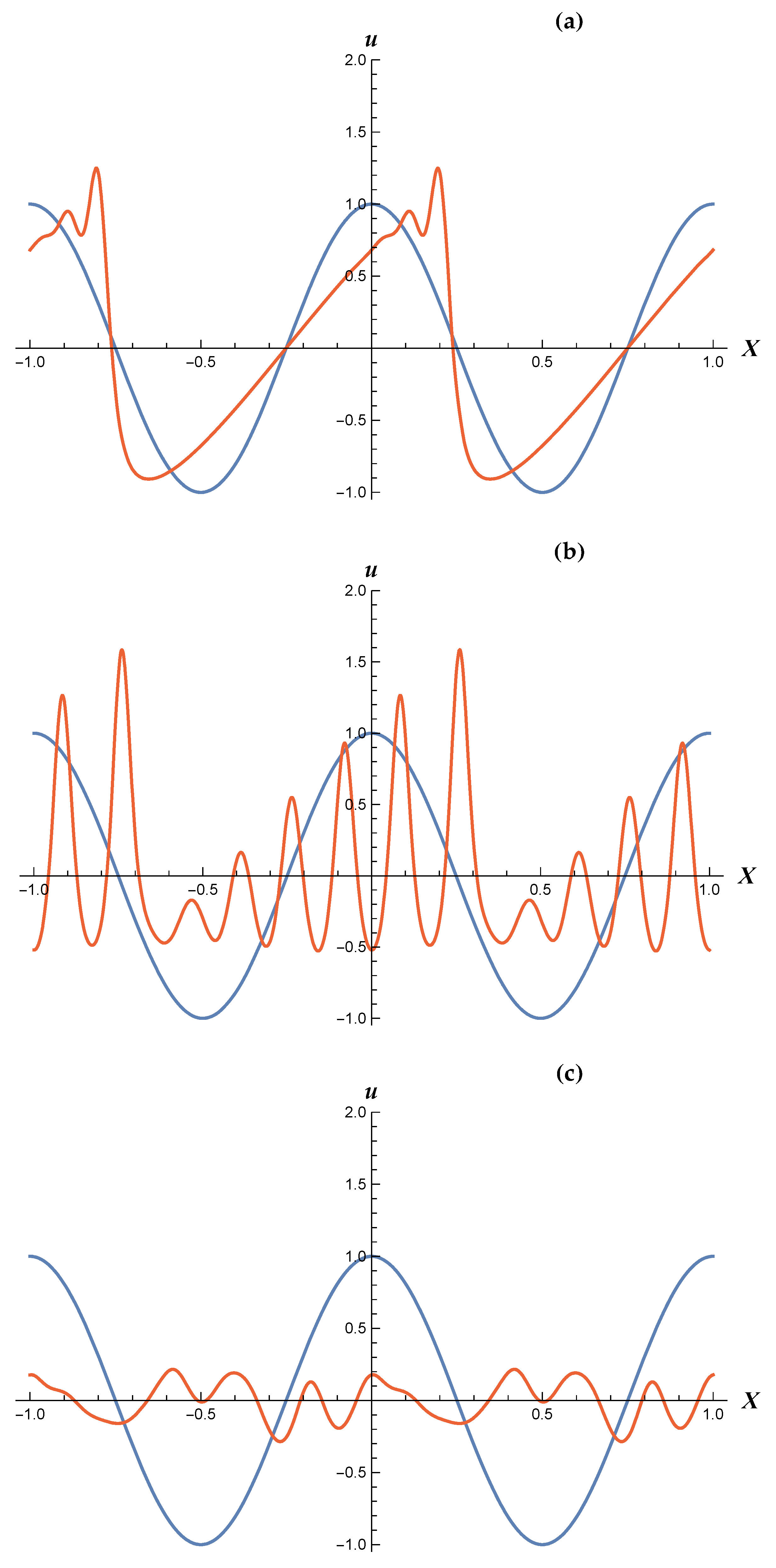
From Figure 1 it is easy to see that, except for attenuation of the profile (caused by the Darcy term) and a slight phase shift, the dKdV profiles are qualitatively similar to those of the classic KdV equation in the setting of IBVP (30). And, as is also true in the case of the latter, reducing (resp. increasing) $a_0$ increases (resp. decreases) the number of pulses seen in Figure 1b.

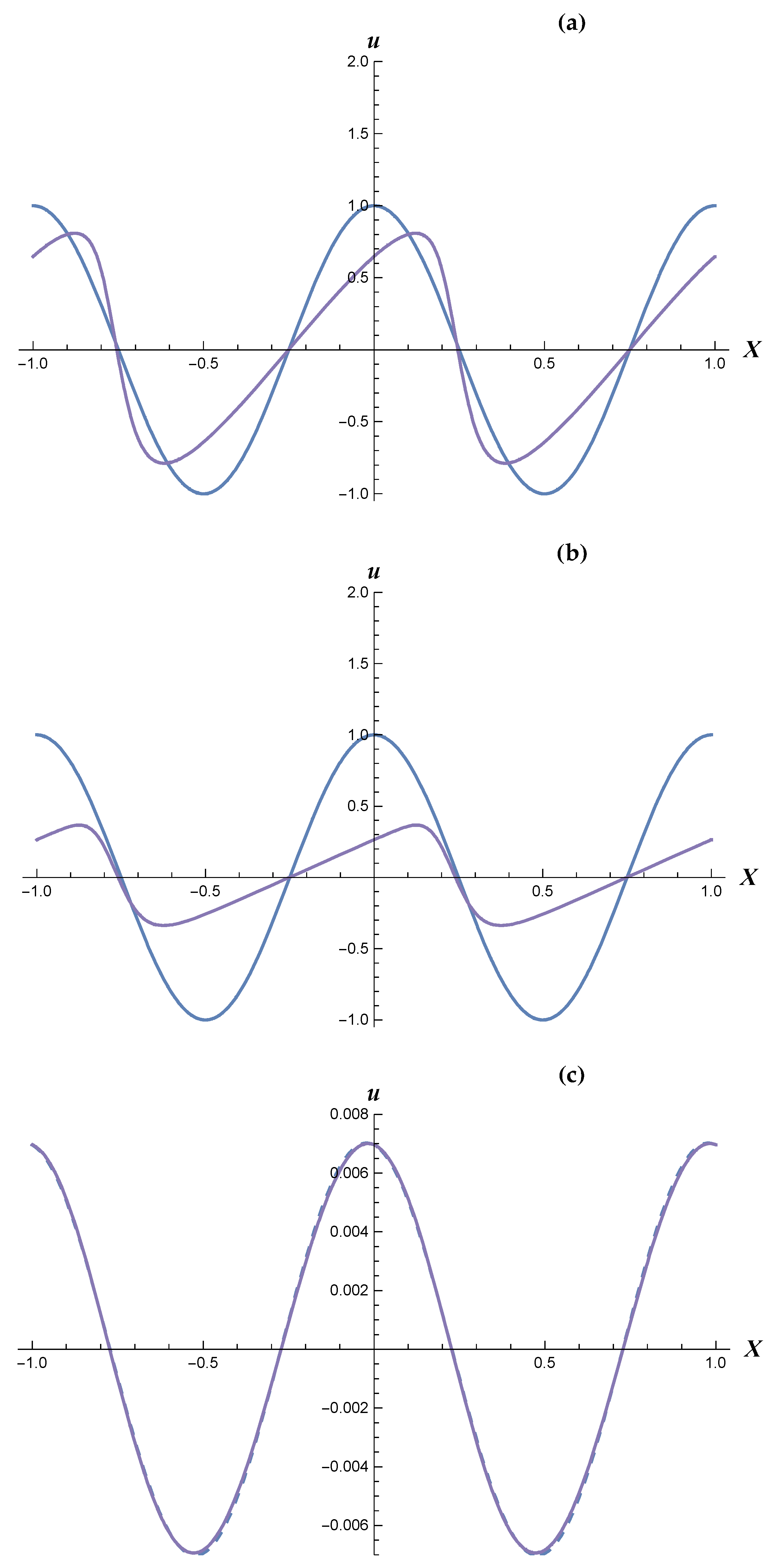
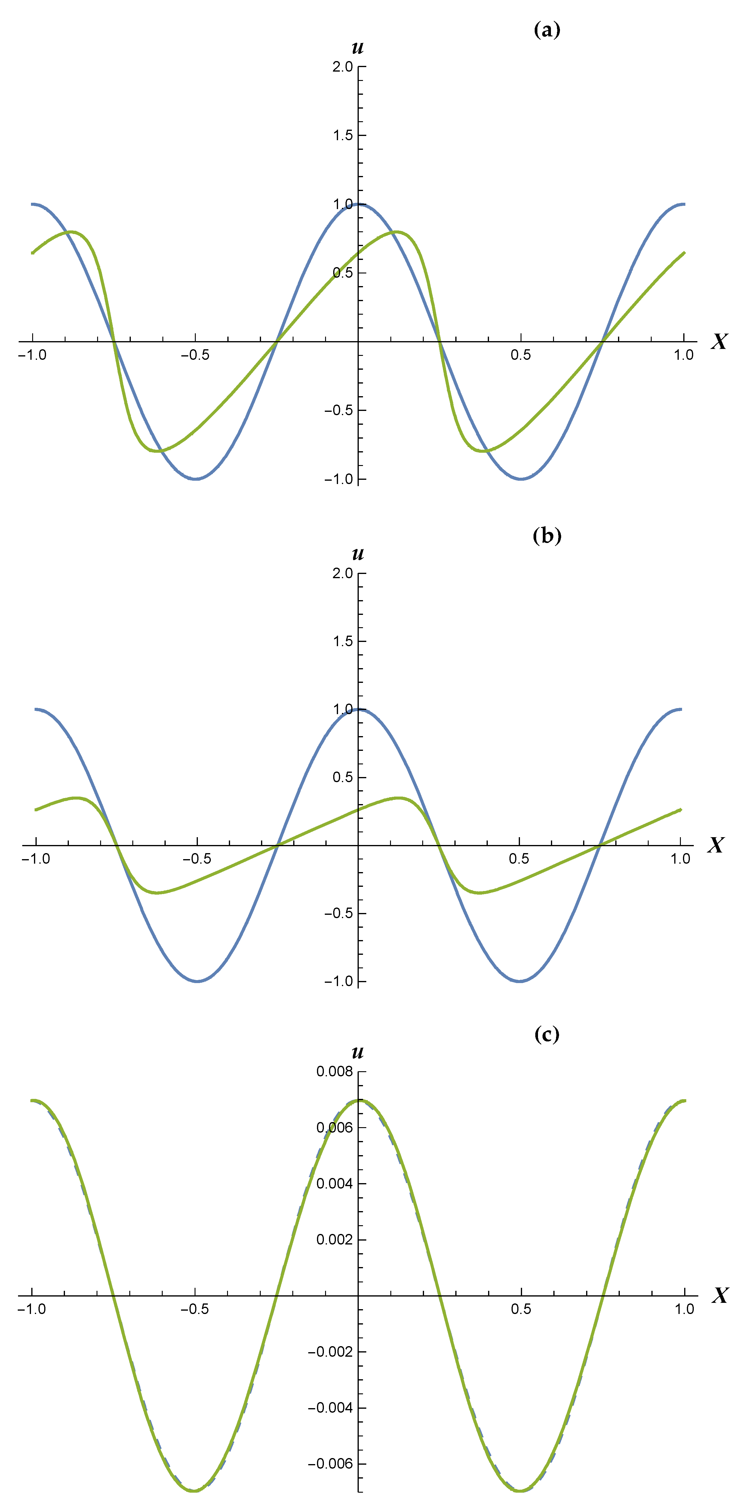
In contrast, the plots shown in Figure 2 and Figure 3 highlight the fact that, like that of the damped Burgers equation, the dBKdV profile suffers attenuation, again due to the Darcy term, and it also develops a “dull sawtooth” appearance as it shocks-up (to the right), but never breaks since $\sigma >0$. More interesting, however, is the fact that for large-T, both the damped Burgers equation and dBKdV profiles are seen to re-assume the periodic form of the IC. As Figure 2c and Figure 3c illustrate, both profiles evolve to become damped, and in the dBKdV case slightly phase-shifted (to the left), versions of the IC given in Equation (30c). This suggests that for sufficiently large values of T, one may employ the approximations $u(X,T)\approx u_{1,2}(X,T)$, where

$$u_{1,2}(X,T):=\left\{\begin{array}{cc}exp[-{♇}_1\left(T\right)]cos[2\pi X+{\psi }_1\left(T\right)],\hfill & \mathrm{dBKdV} \mathrm{equation}\hfill \\ exp[-{♇}_2\left(T\right)]cos[2\pi X+{\psi }_2\left(T\right)],\hfill & \mathrm{damped} \mathrm{Burgers} \mathrm{equation}\hfill \end{array}\right.\hspace{1em}(T\gg T_B^{*}),$$

(31)

and where we require ${♇}_{1,2}\left(T\right)>0$. Comparing the blue-broken curve in Figure 2c with its counterpart in Figure 3c we see that ${♇}_2\left(20T_B^{*}\right)>{♇}_1\left(20T_B^{*}\right)>0$ while ${\psi }_1\left(20T_B^{*}\right)>{\psi }_2\left(20T_B^{*}\right):=0$; here, for simplicity, we have assumed ${♇}_{1,2}\left(T\right)$ and ${\psi }_{1,2}\left(T\right)$ to be linear functions of T. In the setting of IBVP (30), then, the presence of the third order (i.e., RRG) term in the dBKdV equation gives rise to both a phase shift and slightly less attenuation vis-à-vis the damped Burgers equation.

While their usefulness may be limited to certain “windows” of T-values, the functions ${♇}_{1,2}\left(T\right)$ and ${\psi }_{1,2}\left(T\right)$ should be constructible based on Equation (31) and numerically generated, large-T, data sets using one of the many data-fitting methodologies found in the literature.

5. The RRG Case with “Artificial” $\mu$

In 1950, von Neumann and Richtmyer (vNR) [23] introduced their artificial viscosity coefficient. In this section, we make use of this celebrated artifice not to regularize numerical schemes used to calculate shock profiles, as was vNR’s aim, but rather to obtain an analytical solution to the poroacoustic version of the piston problem (Unlike Ref. [23], wherein Lagrangian coordinates were used, in this communication we employ the Eulerian description; see, e.g., (Ref. [24], §V-D-1) wherein vNR’s system is recast under the latter.).

To this end, we return to the RRG case of System (3) and assume that

$$\mu \propto {\alpha }^2\varrho \left|u_x\right|,$$

(32)

but continue to regard $\tilde{\mu }$ as a positive constant. Here, we have expressed the length-scale factor in vNR’s artificial viscosity coefficient as $\alpha$, instead of some grid spacing $\Delta x$.

For simplicity, we now assume that the porous solid in question is comprised of packed beds of rigid solid spheres, all of radius $r(>0)$, which are fixed in place. For such a configuration, the permeability is given by the well known Kozeny–Carmen relation [4]:

$$K=\frac{r^2{\chi }^3}{45{(1-\chi )}^2}.$$

(33)

As these spheres are scatters of acoustic waves, we take $\alpha$ to be proportional to the characteristic length now associated with our dual-phase medium; i.e., we take $\alpha =b_{1}r$, where $b_1(>0)$ is an “adjustable” (dimensionless) constant ([24], p. 233).

If, moreover, we limit our focus to kink-type waveforms, as physical intuition suggests, and have the piston located at $x=-\infty$ and moving to the right along the x-axis, then $u_x<0$ and Equation (32) becomes

$$\mu =-b_1^2{r}^2\varrho {\varphi }_{xx},$$

(34)

where we have used the relation $u={\varphi }_x$. Returning to our dimensionless variables, and once again applying the finite-amplitude approximation, it is readily established that, under the aforementioned assumptions, the following (simpler) weakly-nonlinear PDE replaces Equation (5) as our bi-directional EoM:

$${\varphi }_{tt}-[1-2ϵ(\beta -1){\varphi }_t]{\varphi }_{xx}+ϵ(1-{\delta }_1){\partial }_t{\left({\varphi }_x\right)}^2=\sigma {\varphi }_{txx}+a_1^2{\varphi }_{ttxx}\hspace{1em}(\mathrm{artificial} \mu ).$$

(35)

In Equation (35), which we observe applies only to the RRG case, we have set $a_1:=b_{1}r\sqrt{2}/L$, where we require that $a_1\sim \mathcal{O}\left(ϵ\right)$, and

$${\delta }_1:=\frac{ϵb_1^{2}45{(1-\chi )}^2}{{\chi }^2}\hspace{1em}(0<{\delta }_1<1),$$

(36)

where the requirement ${\delta }_1\in (0,1)$ implies that $b_1$ must satisfy the inequality

$$0<b_1<\frac{1}{3\sqrt{5ϵ}}\left(\frac{\chi }{1-\chi }\right).$$

(37)

Assuming the gas at $x=+\infty$ is in its equilibrium state, and thus motionless, and observing that in the present context $U_{\mathrm{p}}$ is the dimensional speed of the piston, we let $\varphi (x,t)=G\left(\eta \right)$, where $\eta =x-v_{1}t$ and the (dimensionless) shock speed $v_1$ is taken to be a positive constant, and then substitute into Equation (35). On integrating once with respect to $\eta$ and then imposing/enforcing the asymptotic conditions $g\to 1,0$ as $\eta \to \mp \infty$, respectively, Equation (35) is reduced to the ODE

$$a_1^2{v}_1{g}^{″}-\sigma g^{\prime }-ϵ{\beta }_{1}g(1-g)=0,$$

(38)

where we note that the resulting constant of integration is zero. In Equation (38), $g\left(\eta \right)=G^{\prime }\left(\eta \right)$, where a prime denotes $\mathrm{d}/\mathrm{d}\eta$; we have defined

$${\beta }_1:=\beta -{\delta }_1,$$

(39)

recalling that $\beta$ is the coefficient of nonlinearity (see Equation (6)); and

$$v_1=\frac{1}{2}ϵ{\beta }_1+\sqrt{1+\frac{1}{4}{ϵ}^2{\beta }_1^2}\hspace{1em}(v_1>1),$$

(40)

which we observe is the positive root of

$$v_1^2-ϵ{\beta }_1{v}_1-1=0.$$

(41)

To apply the solution methodology employed in (Ref. [2], §2) to Equation (38), the following condition must be satisfied:

$$25a_1^2(v_1^2-1)=6{\sigma }^2.$$

(42)

In (Ref. [2], §2), satisfying Equation (42) required that the value of the Mach number be fixed, a constraint which clearly limits the usefulness of the TWSs presented in that article. Here, however, we shall use this restriction to our advantage; specifically, in the following sense: Since the value of $\tilde{\mu }$ for a given poroacoustic flow is, in general, not known, and we are seeking a kink-type TWS, then the only possible solution of Equation (42) in the present context is

$$\sigma =5a_1\sqrt{\frac{v_1^2-1}{6}}\hspace{1em}\Rightarrow \hspace{1em}\tilde{\mu }=\frac{5{\varrho }_0{b}_{1}r}{\chi }\sqrt{\frac{{\mathfrak{v}}_1^2-c_0^2}{3}},$$

(43)

where we observe that ${\mathfrak{v}}_1=v_1{c}_0$ is the dimensional shock speed and, moreover, that $v_1>1$ implies ${\mathfrak{v}}_1>c_0$.

On imposing the usual wave front condition $g\left(0\right)=1/2$, but otherwise referring the reader to (Ref. [2], §2) for details regarding its derivation, the TWS we seek is

$$g\left(\eta \right)=\frac{1}{4}{\mathrm{sech}}^2\left(\frac{27\eta }{16{\lambda }_1}+\mathcal{K}\right)+\frac{1}{2}\left[1-\tanh \left(\frac{27\eta }{16{\lambda }_1}+\mathcal{K}\right)\right],$$

(44)

where $\mathcal{K}={\tanh }^{-1}\left(-1+\sqrt{2}\right)$. Letting ${\lambda }_1={\ell }_1/L$ denote the dimensionless shock thickness (Recall Equation (2)) admitted by Equation (44), it is easily established that

$${\lambda }_1=\frac{135a_1^2{v}_1}{8\sigma }=\frac{81a_1{v}_1}{4\sqrt{6(v_1^2-1)}}\hspace{1em}\Rightarrow \hspace{1em}{\ell }_1=\frac{81{\mathfrak{v}}_1{b}_{1}r}{4\sqrt{3({\mathfrak{v}}_1^2-c_0^2)}},$$

(45)

where ${\ell }_1$ is the corresponding dimensional shock thickness. Also, with regard to computing ${\lambda }_1$, it should be noted that $g^{″}\left({\eta }^{*}\right)=0$, where ${\eta }^{*}(<0)$ is given by

$${\eta }^{*}=\frac{10a_1^2{v}_1\left[{\tanh }^{-1}\left(1/3\right)-\mathcal{K}\right]}{\sigma },$$

(46)

and where it should also be noted that $g\left({\eta }^{*}\right)=5/9$.

The usefulness of Equation (45) might be ascertained as follows. Assume that ${\mathfrak{v}}_1$ and ${\ell }_1$ can both be determined, either directly or indirectly, from experimental measurements and, moreover, that both are (at most) slowly varying functions of time. With ${\mathfrak{v}}_1$ known, $b_1$ can, of course, be computed using Equations (36), (39) and (40). If this (inferred) value of $b_1$ satisfies the inequality in Equation (37), $a_1\sim \mathcal{O}\left(ϵ\right)$ is also satisfied, and the measured value of ${\ell }_1$ is in agreement with that computed from Equation (45) over, say, some span of time $t\in \mathcal{T}$, then we can expect Equation (45) to prove useful as an approximation within the transition region of our kink-type traveling wave profile for $t\in \mathcal{T}$.

6. Discussion: Possible Follow-On Studies

In addition to gaining a better understanding of how the solution of IBVP (30) behaves for large-T, in particular, determining to what extent (if any) the recurrence behavior seen in Figure 2c and Figure 3c is related to the functional form of a given IC, future work on poroacoustic RRG theory could included the use of homogenization methods in problems wherein K and/or $\chi$ vary with position. Other possible extensions include the poroacoustic generalization of the study carried out in Ref. [25], wherein $\alpha$ was taken to be a function of ${\left(u_x\right)}^2$, and also the case in which $\tilde{\mu }$ is a power-law function of the shear rate tensor. Follow-on work might also include the study of poroacoustic signaling problems involving sinusoidal and/or shock input signals, as well as problems in which changes in entropy and temperature are taken into account.

References

- Rubin, M.B.; Rosenau, P.; Gottlieb, O. Continuum model of dispersion caused by an inherent material characteristic length. J. Appl. Phys. 1995, 77, 4054–4063. [Google Scholar] [CrossRef]
- Jordan, P.M.; Keiffer, R.S.; Saccomandi, G. A re-examination of weakly-nonlinear acoustic traveling waves in thermoviscous fluids under Rubin–Rosenau–Gottlieb theory. Wave Motion 2018, 76, 1–8. [Google Scholar] [CrossRef]
- Burmeister, L.C. Convective Heat Transfer, 2nd ed.; Wiley: Hoboken, NJ, USA, 1993; §2.8. [Google Scholar]
- Nield, D.A.; Bejan, A. Convection in Porous Media, 5th ed.; Springer: Berlin/Heidelberg, Germany, 2017; Chapter 1. [Google Scholar]
- Straughan, B. Stability and Wave Motion in Porous Media; Applied Mathematical Sciences; Springer: Berlin/Heidelberg, Germany, 2008; Volume 165. [Google Scholar]
- Morduchow, M.; Libby, P.A. On a complete solution of the one-dimensional flow equations of a viscous, heat-conducting, compressible gas. J. Aeronaut. Sci. 1949, 16, 674–684, 704. [Google Scholar] [CrossRef]
- Thompson, P.A. Compressible-Fluid Dynamics; McGraw–Hill: New York, NY, USA, 1972. [Google Scholar]
- Keiffer, R.S.; McNorton, R.; Jordan, P.M.; Christov, I.C. Dissipative acoustic solitons under a weakly-nonlinear, Lagrangian-averaged Euler-α model of single-phase lossless fluids. Wave Motion 2011, 48, 782–790. [Google Scholar] [CrossRef]
- Beyer, R.T. The parameter B/A. In Nonlinear Acoustics; Hamilton, M.F., Blackstock, D.T., Eds.; Academic Press: Cambridge, MA, USA, 1998; pp. 25–39. [Google Scholar]
- Crighton, D.G. Model equations of nonlinear acoustics. Ann. Rev. Fluid Mech. 1979, 11, 11–33. [Google Scholar] [CrossRef]
- Ott, E.; Sudan, R.N. Damping of solitary waves. Phys. Fluids 1970, 13, 1432–1434. [Google Scholar] [CrossRef]
- Karpman, V.I. Soliton evolution in the presence of perturbation. Phys. Scr. 1979, 20, 462–478. [Google Scholar] [CrossRef]
- Leibovich, S.; Randall, J.D. On soliton amplification. Phys. Fluids 1979, 22, 2289–2295. [Google Scholar] [CrossRef]
- Zabusky, N.J.; Kruskal, M.D. Interaction of “Solitons” in a collisionless plasma and the recurrence of initial states. Phys. Rev. Lett. 1965, 15, 240–243. [Google Scholar] [CrossRef] [Green Version]
- Rossmanith, D.; Puri, A. Recasting a Brinkman-based acoustic model as the damped Burgers equation. Evol. Equs. Control Theory 2016, 5, 463–474. [Google Scholar] [CrossRef] [Green Version]
- Nimmo, J.J.; Crighton, D.G. Bäcklund transformations for nonlinear parabolic equations: The general results. Proc. R. Soc. Lond. A 1982, 384, 381–401. [Google Scholar]
- Malfliet, W. Approximate solution of the damped Burgers equation. J. Phy. A Math. Gen. 1993, 26, L723–L728. [Google Scholar] [CrossRef]
- Ciarletta, M.; Straughan, B. Poroacoustic acceleration waves. Proc. R. Soc. A 2006, 462, 3493–3499. [Google Scholar] [CrossRef]
- Jordan, P.M. Growth and decay of acoustic acceleration waves in Darcy-type porous media. Proc. R. Soc. A 2005, 461, 2749–2766. [Google Scholar] [CrossRef]
- Jordan, P.M. Poroacoustic solitary waves under the unidirectional Darcy–Jordan model. Wave Motion 2020, 94, 102498. [Google Scholar] [CrossRef]
- Crighton, D.G. Propagation of finite-amplitude waves in fluids. In Handbook of Acoustics; Crocker, M.J., Ed.; Wiley-Interscience: Hoboken, NJ, USA, 1998; Chapter 17. [Google Scholar]
- Logan, J.D. An Introduction to Nonlinear Partial Differential Equations, 2nd ed.; Wiley-Interscience: Hoboken, NJ, USA, 2008. [Google Scholar]
- Von Neumann, J.; Richtmyer, R.D. A method for the numerical calculation of hydrodynamic shocks. J. Appl. Phys. 1950, 21, 232–237. [Google Scholar] [CrossRef]
- Roache, P.J. Computational Fluid Dynamics; Hermosa Publishers: Albuquerque, NM, USA, 1972. [Google Scholar]
- Jordan, P.M.; Saccomandi, G. Compact acoustic travelling waves in a class of fluids with nonlinear material dispersion. Proc. R. Soc. A 2012, 468, 3441–3457. [Google Scholar] [CrossRef]
- Leibovich, S.; Cornell University, New York, NY, USA. Personal communication, 22 May 2018.
Figure 1.
The dKdV case of IBVP (30). (a–c) correspond to , , and , respectively, where . Red curves: u vs. X for , , , , and . Blue curves: IC given in Equation (30c).
Figure 2.
The dBKdV case of IBVP (30). (a–c) correspond to , , and , respectively, where . Purple curves: u vs. X for , , , , and . Blue curves (solid): IC given in Equation (30c). Blue-broken curve: vs. X (see Equation (31)), where we have set and based on a series of trial-and-error “visual fits”.
Figure 3.
The damped Burgers equation case of IBVP (30). (a–c) correspond to , , and , respectively, where . Green curves: u vs. X for , , , , and . Blue curves (solid): IC given in Equation (30c). Blue-broken curve: vs. X (see Equation (31)), where we have set and based on a series of trial-and-error “visual fits”.
© 2020 by the author. Licensee MDPI, Basel, Switzerland. This article is an open access article distributed under the terms and conditions of the Creative Commons Attribution (CC BY) license (http://creativecommons.org/licenses/by/4.0/).
Share and Cite
MDPI and ACS Style
Jordan, P.M. Poroacoustic Traveling Waves under the Rubin–Rosenau–Gottlieb Theory of Generalized Continua. Water 2020, 12, 807. https://doi.org/10.3390/w12030807
AMA Style
Jordan PM. Poroacoustic Traveling Waves under the Rubin–Rosenau–Gottlieb Theory of Generalized Continua. Water. 2020; 12(3):807. https://doi.org/10.3390/w12030807
Chicago/Turabian StyleJordan, Pedro M. 2020. "Poroacoustic Traveling Waves under the Rubin–Rosenau–Gottlieb Theory of Generalized Continua" Water 12, no. 3: 807. https://doi.org/10.3390/w12030807
Note that from the first issue of 2016, this journal uses article numbers instead of page numbers. See further details here.