Managing Water Quality in Intermittent Supply Systems: The Case of Mukono Town, Uganda

Abstract

Intermittent water supply networks risk microbial and chemical contamination through multiple mechanisms. In particular, in the cities of developing countries, where intrusion through leaky pipes are more prevalent and the sanitation systems coverage is low, contaminated water can be a public health hazard. Although countries using intermittent water supply systems aim to change to continuous water supply systems—for example, Kampala city is targeting to change to continuous water supply by 2025 through an expansion and rehabilitation of the pipe infrastructure—it is unlikely that this transition will happen soon because of rapid urbanisation and economic feasibility challenges. Therefore, water utilities need to find ways to supply safe drinking water using existing systems until gradually changing to a continuous supply system. This study describes solutions for improving water quality in Mukono town in Uganda through a combination of water quality monitoring (e.g., identifying potential intrusion hotspots into the pipeline using field measurements) and interventions (e.g., booster chlorination). In addition to measuring and analyses of multiple chemical and microbial water quality parameters, we used EPANET 2.0 to simulate the water quality dynamics in the transport pipeline to assess the impact of interventions.

1. Introduction

Intermittent water supply systems represent a range of water supply services that supply water to consumers for less than 24 h per day or not at sufficiently high pressures [1]. Such systems are typical in developing countries, with more than 1.3 billion people in at least 45 low- and middle-income countries reportedly receiving water through intermittent systems [2,3,4]. It is generally considered that intermittent water supply systems are not an ideal method of supply and do not constitute the best solution [5]. Where such systems are poorly maintained and have leaky pipe infrastructure, contamination can intrude into the water distribution system when pipes are at low or zero pressure. This could be through infrastructure deficiencies (e.g., holes and cracks in some pipes due to aging and deterioration) or break flows through cross connections (a plumbed connection between a potable water supply and a non-potable water source) and this could happen through events that are persistent or temporary [6,7,8,9]. In particular, contamination of pathogenic microorganisms such as E. coli in water cause various diseases [10]. However, intermittent water supply is being used by many water utilities to address water shortages (e.g., in drought conditions) or increasing demand, without considering long-term alternative solutions [1]. Although essential, transitioning from intermittent water supply systems to continuous water supply systems is often difficult for utilities [11,12] and needs to be done in a cost-effective way, combining improved operations with targeted capital works [1].

In Uganda Vision 2040 [13], the government aims “to improve the health, sanitation, hygiene, promote commercial and low consumption industrial setups, Government (sic) will construct and extend piped water supply and sanitation systems to all parts of the country”. To accomplish this, the Ministry of Water outlines “improved water quality” and “reliable water quantity” as actionable targets for 2040 [14]. The planned transitions are even more ambitious for Kampala and target 2025 with the Kampala Water Project to rehabilitate the distribution network and extend water treatment capacity to meet all needs [14], in a bid to attain Sustainable Development Goal (SDG) 6, which focuses on sustainable access to clean water and sanitation. This means it will take up to 20 years to change all water supply systems in Uganda to new continuous systems. However, safe water quality is required under intermittent water supply systems until continuous supply goals are achieved.

In previous research, residual chlorine values in the Kampala water distribution system were investigated to assess the potential of recontamination [15]. Although Ecuru et al. [15] were only concerned with physicochemical water quality parameters (temperature, pH, turbidity, colour, ammonia, Fe²⁺, and free chlorine), they were able to show low levels of residual chlorine compared to the minimum standard requirements. However, microbial water quality parameters were missing. In addition, interventions on how to maintain the level of residual chlorine in the water distribution systems, as well as parameters for other water pollutants were also not investigated.

In this manuscript, we assess multiple chemical and microbial water quality parameters in the Kampala water distribution system and examine the impact on water quality in Mukono town because of low pressure and leaky pipe infrastructure under intermittent water supply systems. The treatment works in Kampala use conventional chlorination as a disinfectant with the aim of maintaining disinfectant residuals throughout the supply network. We, therefore, measure residual chlorine levels at different parts of the water distribution system as an indicator for remaining disinfection potential and assess multiple water quality parameters, including microbial water quality (e.g., E. coli), to examine the water quality from the treatment plant to the very end of the network. The study is based on sample data collected at multiple sampling points between Ggaba II (water treatment plant) and Mukono town, via the centre of Kampala. This study considers pH, colour, turbidity, nitrate, nitrite, ammonia, sulphate, E. coli, total coliform, COD (Chemical Oxygen Demand) and chlorine because these parameters are related to water contamination by chemical and microbial pollutants that can cause health hazards [15]. Based on this assessment, we also propose booster chlorination in the supply reservoirs to reduce the microbial risk within the existing intermittent water supply system. By coupling the modelling of the distribution network hydraulics and chlorine decay processes in EPANET 2.0 [16], with residual chlorine levels from measurements, we propose feasible booster chlorine levels to achieve minimum standards for residual chlorine at all consumption nodes.

2. Materials and Methods

2.1. Current State of Site and Its Water Distribution System

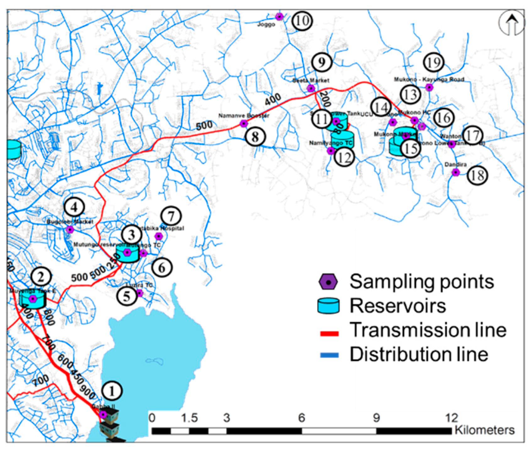
Our study focuses on Mukono, a town in the north east of Kampala with a population of 664,300 (in 2018) [17]. Water is supplied to Mukono for an average of 20 to 24 h per day to all customers and sourced from Lake Victoria, as with most towns in Uganda [4]. Water pumped up from Lake Victoria is supplied to customers after a treatment process that includes coagulation, flocculation, sedimentation, gravel and sand filtration, disinfection with chlorine gas and pH adjustment by soda [4,18]. The design capacity of Ggaba II is 80,000 m³/day with an average production of about 70,252 m³/day [19]. Water is transmitted to the primary reservoirs of Muyenga, Seeta and Mukono (see Figure 1 and

Table 1. The number and name of each sampling location as well as their respective elevation in the Kampala water distribution system (elevation data was acquired from the National Water and Sewerage Corporation (NWSC)’s GIS (Geographic Information System) data set).

Number	Name of Place	Elevation (m)	Number	Name of Place	Elevation (m)
1	Ggaba II	1126	11	Seeta tank lower	1170
2	Muyunga Tank E	1232	12	Namilyango Trading center	1196
3	Mutungo reserver	1228	13	Mukono Health Center	1168
4	Bugorobi Market	1172	14	Mukono UCU	1256
5	Luzira Trading Center	1146	15	Mukono tank A+B	1164
6	Mutungo Trading center	1168	16	Mukono Market	1240
7	Butabika Hospital	1168	17	Mukono Wantoni	1176
8	Namanve Booster	1134	18	Mukono Dandira	1160
9	Seeta market	1182	19	Mukono Kayunga Road	1172
10	Bukerere Joggo	1202

). The distribution and transmission pipes range in diameter from 50 to 900 millimetres.

2.2. Sampling Locations

This study was conducted on the Kampala water supply line from Ggaba II to Mukono town, via Kampala, in Uganda during January 2019. Kampala is the capital city of Uganda. This study focused on main points (19 sites) of the water supply system, such as the water treatment plant (Ggaba II), water storage tanks (supply reservoirs) and end user taps at various locations (a hospital, a market, a trading centre, a pump station and a university). The name of places, locations and elevations are shown in Figure 1 and listed in Table 1.

2.3. Choice of Water Quality Parameters

To assess water quality, twelve water parameters were selected for the analysis and simulation of the supply system (

Table 2. Measurement kit and device to measure water quality of tap water.

Measurement Items	Measurement Devices
E. coli, Total coliform	Compact Dry EC Nissui for Coliform and E. coli
Free chlorine, COD, Ammonia, Nitrate, Nitrite, Sulphate, Turbidity	Photometer PF-12Plus and NANOCOLOR tube test

): free chlorine, E. coli, total coliform, COD, ammonia, nitrate, nitrite, sulphate, turbidity, pH, water age and water pressure. All samples were collected and tested within the standard 30-h holding time [20].

These parameters were chosen for multiple reasons. For example, changes in residual chlorine are linked with pollution by chemicals like ammonia and biofilm growth; chlorine reactions with corrosion products and COD could most likely explain low residual chlorine levels at the end of the network, where water age can be high [21]. The low residual chlorine levels in the Mukono reservoir and areas that follow are more likely due to this reason. Higher turbidity levels are often associated with higher levels of viruses, parasites and some bacteria [22]. There can be correlations between water age and chlorine levels [21]. Exposure to extreme pH values results in irritation to the eyes, skin, and mucous membranes [23]. Careful attention to pH control is necessary at all stages of water treatment to ensure satisfactory water purification and disinfection [24]. For effective disinfection with chlorine, the pH should preferably be less than eight and pH levels that are too low can affect the degree of corrosion of metals [23]. Maintaining continuous optimal water pressure in drinking water distribution systems can protect water from contamination as it flows to consumer taps [25,26]. Sulphate is one of the major dissolved components of rain. High concentrations of sulphates in drinking water can have a laxative effect [27]. Ammonia, nitrite and nitrate can cause algae growth [28] and can be indicators of pollution from agriculture and anthropogenic sources. Ammonia is an important indicator of faecal pollution [29]. Nitrite and nitrate have toxic effects for infants under three months of age and so require monitoring [30].

2.4. Sampling Methods, Measurement Items and Analysis

We followed recommended methods, also used by the National Water and Sewerage Corporation (NWSC), to collect samples. Samples for chemical analysis were collected in clean 500 ml plastic bottles. After flushing the taps for more than 10 seconds in order to clean the faucet, the sampling bottle was rinsed three times with the same water source as the sample before sampling. Collected samples were brought back to a laboratory using a cold storage case to keep them at low temperatures (at under 10 ℃) to prevent bacterial growth during transport [20].

The measurement items and devices are listed in Table 2. Free chlorine was tested twice on-site using Photometer PF-12^Plus (MACHEREY-NAGEL, Düren, Germany) and the NANOCOLOR tube test (MACHEREY-NAGEL, Düren, Germany) by following the procedure of NANOCOLOR tube test. The samples for E. coli and total coliform were tested by incubating for 24 h at 35 ℃ ± 2 in an incubator by Compact Dry EC Nissui for coliform and E. coli detection (Nissui, Tokyo, Japan) by following the protocol for Compact Dry EC Nissui for coliform and E. coli detection. Nitrite, nitrate, sulphate, ammonia and turbidity were tested twice for each sample by Photometer PF-12^Plus and the NANOCOLOR tube test in the laboratory by following the procedure of the NANOCOLOR tube test, and were validated with pH data from January 2019 using records from internal GIS and measurement databases maintained by the operations team at NWSC. Water age and water pressure were assessed using EPANET simulations. Measurement ranges for parameters were selected to include recommended standards by WHO [24], the Ministry of the Environment Government of Japan [31], or as in Wang et al. [32] and Kumpel et al. [8] (See

Table 3. Measured parameters of water quality, the standards of water quality and range of photometer used.

Measurement Items	Measurement Standard	Range of Photometer
Free chlorine	0.5 mg/L (0.2–1.0) [24]	-
E. coli	0 (CFU/100mL) [24]	-
Total coliform	0 (CFU/100mL) [24]	-
COD	≤5 mg/L [31]	3 to 150 mg/L
Ammonia	≤1.5 mg/L [24]	0.04 to 2.30 mg/L
Nitrite	≤3 mg/L [24]	0.3 to 22.0 mg/L
Nitrate	≤50 mg/L [24]	0.1 to 4.0 mg/L
Sulphate	≤250 mg/L [24]	40 to 400 mg/L
Turbidity	≤5 NTU [24]	1 to 1000 NTU
pH	6 ≤ pH ≤ 9 [24]	-
Water age	≤5.7 days (136.8 h) [32]	-
Water pressure	≥17 psi [8]	-

).

2.5. Water Quality Modelling

EPANET 2.0 is a computer program that can perform extended period simulation of hydraulic and water quality behaviour within pressurised pipe networks with pipes, nodes (pipe junctions), pumps, valves and storage tanks or reservoirs [16].

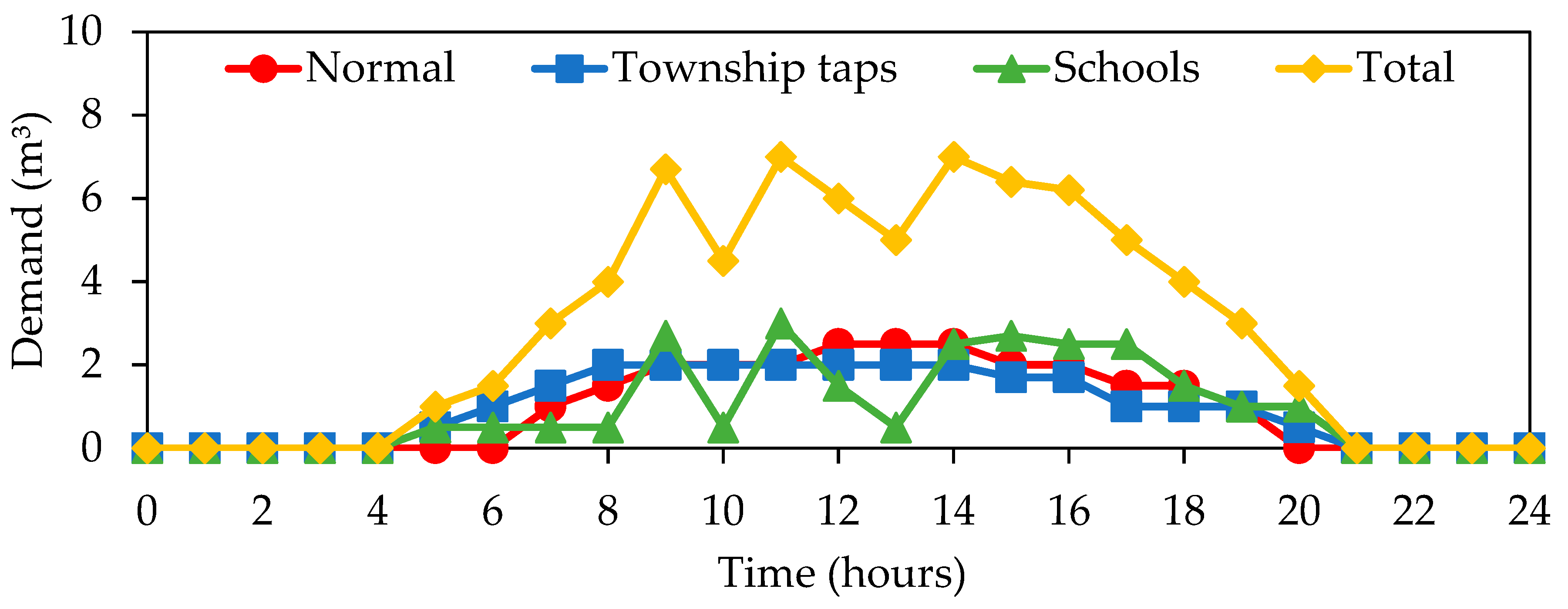
This paper used EPANET 2.0 to simulate chlorine decay, water age and pressure levels in the distribution network modelled. The pipe length and diameter data of the distribution network are shown in Figure 1 and presented in detail in

Table 4. Pipe length, diameter and roughness of water distribution lines from Ggaba II to Mukono. The name of the numbered sites or nodes is as shown in Table 1.

Pipe Name (from node No. x to y)	Pipe Length (m)	Pipe Diameter (mm)	Pipe Roughness
1 to 2	5260	800	140
2 to 3	4210	500	140
3 to 4	2700	100	140
3 to 5	1740	100	140
3 to 6	660	100	140
6 to 7	1340	100	140
3 to 8	11700	500	140
8 to 11	4710	400	140
11 to 9	1680	200	140
11 to 12	1230	100	140
9 to 10	3260	100	140
9 to15	6920	400	140
15 to 13	1220	100	140
15 to 14	710	100	140
15 to 16	1530	100	140
16 to 17	1100	100	140
17 to 18	860	100	140
13 to 16	1240	100	140
13 to 19	1100	100	140

. The considered part of the distribution network consists of five different pipe diameters and different lengths per diameter, which were all derived from the GIS dataset maintained by the National Water and Sewage Corporation (NWSC). Pipe roughness (Table 4) was derived using recommend values by Swierzawski (2000) for the material types and age [33], which are assumed to be the same for all pipe sections here. Future work can consider calibrating the roughness of the pipes, which may be different as thw pipes age. Three typical demand patterns in Kampala water distribution systems were generated to model the end-user demand for water in this study (Figure 2) [18]. Each pattern was applied based on the Republic of Uganda Ministry of water and environment’s manual on demand patterns for Ugandan urban water use (2013), also shown in

Table 5. Demand pattern for each sampling points.

No.	Pattern	No.	Pattern
1	-	11	-
2	-	12	Township taps
3	-	13	Normal
4	Township taps	14	School
5	Township taps	15	-
6	Township taps	16	Township taps
7	Township taps	17	Normal
8	-	18	Normal
9	Township taps	19	Normal
10	Normal

[18]. EPANET was run to simulate water quality parameters for 168 h (i.e., 7 days).

2.5.1. Headloss in Pipes (Hazen–Williams Formula)

In this study, the Hazen–Williams formula was used to model frictional losses in the hydraulic model. The headloss across a pipe, per 100 feet of pipe, is given as:

$$Pd=\frac{4.52\times Q^{1.85}}{C_{hw}{}^{1.85}\times d^{4.87}}$$

(1)

where Q = flow rate (gpm or Lpm), $C_{hw}$. = roughness coefficient, dimensionless, d = inside pipe diameter, in mm. The total head drop in the system (psi) as a function of the pipe length L (ft) is given as [16]:

$$Td=0,002082L\times \frac{{100}^{1.85}}{C}\times \frac{Q^{1.85}}{d^{1.8655}}$$

(2)

with velocity (V), flow rate (Q) and friction headloss (f) are computed as follows:

$$V=1.318\times C_{hw}\times R^{0.63}\times S^{0.54}$$

(3)

$$Q=0.849\times C_{hw}\times A\times R^{0.63}\times S^{0.54}$$

(4)

$$f=\frac{6.05\times Q^{1.85}}{C_{hw}{}^{1.85}\times d^{4.78}}$$

where S = the slope of the energy line (head loss per length of pipe, unitless), f = friction head loss in ft. hd./100 ft. of pipe (m per 100m), Pd = pressure drop (psi/100 feet of pipe), R = hydraulic radius, feet (m), V = velocity (feet per second), and A = cross section area, in (mm²).

2.5.2. Chlorine Decay Kinetics

There are two main reasons why residual chlorine decays through reactive processes [34,35]. One reason can be external contamination, which happens often during pipeline breaks and maintenance operations, and the second is the decay with time through reaction with natural organic matter in the bulk water. The chlorine decay model [34,35,36,37] that is included in EPANET 2.0 [16] and used within our water quality analysis accounts for both bulk and wall reactions, with a limited growth on the ultimate concentration of the decaying substance, as follows:

$$r=k_b\left(C_L-C\right)C^{\left(n-1\right)}.$$

(5)

where r is the rate of reaction (mass/volume/time), kb is the reaction constant, C is the reactant concentration (mass/volume), n is the reaction order, and C_L is the limiting concentration. Chlorine reactive decay in the bulk flow within the pipe is adequately modelled by a simple first-order reaction (n = 1, k_b = 0.849/s, C_L = 0 are used here [16]). The rate of the reactant reactions that happen at pipe walls are related to the reactant’s concentration in the bulk, modelled as:

$$r_2=\left(A/V\right)k_w{C}^n$$

(6)

where r₂ is the rate of reaction (mass/volume/time), A/V is the surface area per unit volume within the pipe which equals (4/pipe diameter), C is the chlorine concentration (mass/volume), n is the kinetics order (1 here), and k_w is the wall reaction rate coefficient (length/time for n=1 and mass/area/time for n=0). The EPANET simulation makes automatic adjustments to account for mass transfer between the bulk flow and the wall, based on the molecular diffusivity of the reactant under study and the Reynolds number of the flow. In the case of zero-order kinetics, which are recommended by the program manual [16], the wall reaction rate cannot be greater than the mass transfer rate, resulting in:

$$r_2=-MIN\left(k_w, k_{f}C\right)\left(2/R\right),$$

(7)

where k_f is the mass transfer coefficient (length/time), C is the chlorine concentration (mass/volume), and R is the pipe radius (length).

Water age was also calculated by EPANET 2.0 and was used to assess the age of each parcel of water in the system, where we have only one source at the treatment plant and the dynamics of service reservoirs (with a complete mixing model, i.e., the MIXED setting for tanks [16]) was employed. A “setpoint booster source” was used to fix the concentration of outflows leaving booster nodes, where the concentration of all inflow reaching the booster nodes was below the outflow chlorine concentration that was set. In this manuscript, Microsoft Office Excel (2016) was used to do the statistical analysis and visualize the results. Error bars were created using standard deviation P function in Microsoft Office Excel (2016).

3. Results and Discussion

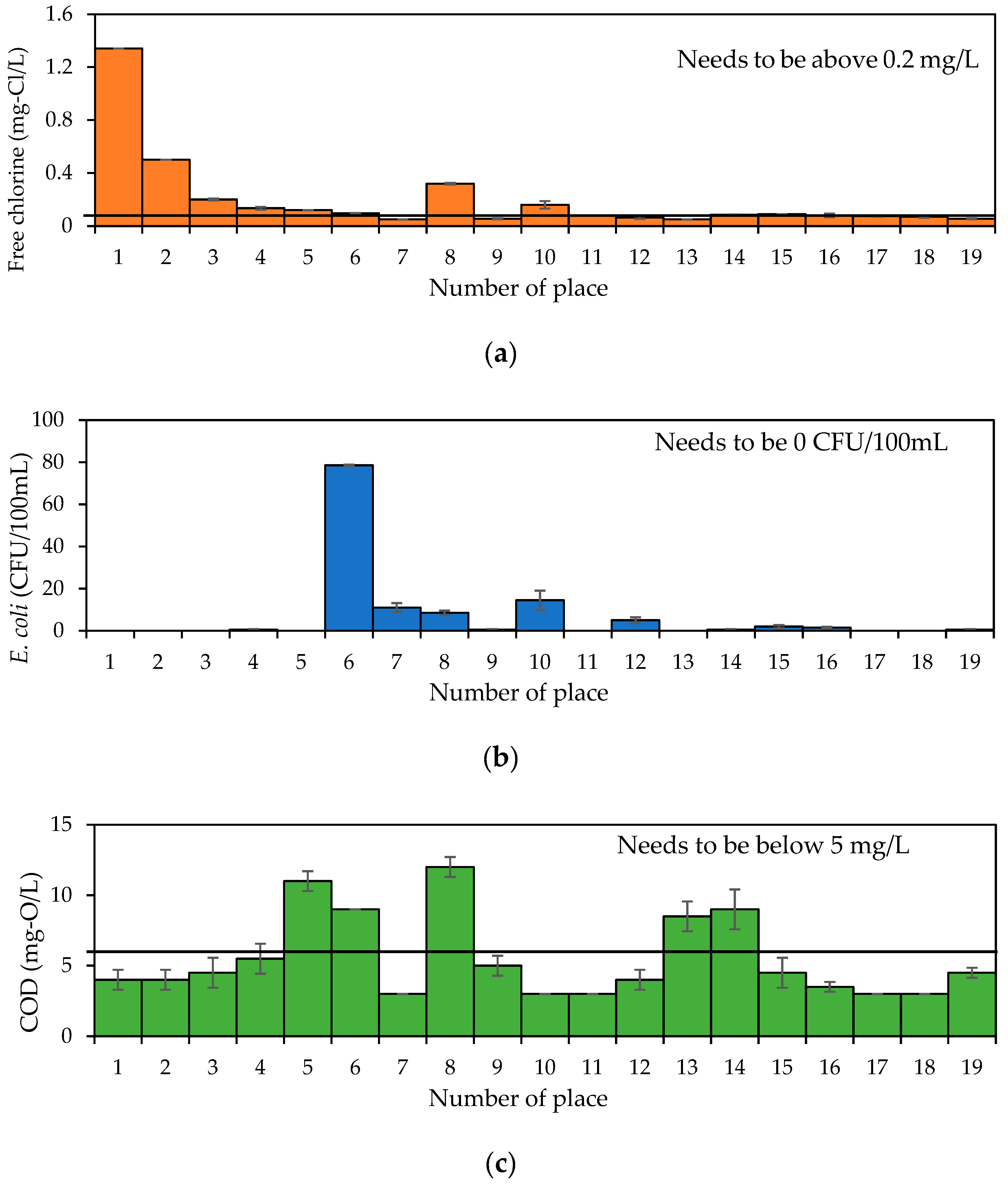
Free chlorine levels measured for samples of the distribution system did not meet the WHO standard of ≥0.2 mg/L [24] at 15 sites. E. coli was detected at 11 sites (other bacteria were not detected). Although the average COD level did not meet the standard of ≤5 mg/L [31] at six locations, there were an additional four sites where one of the samples exceeded this threshold, i.e., locations three, four, nine and 15 in Figure 3c. Therefore, with more measurements, it is possible that more locations may have higher COD values.

The average pH value in the water supply system was 7.1, the lowest was 6.8 (at Namanve booster) and the highest at 7.4 in Mukono market, which all meet the WHO standard set in [24]. Sulphate was detected at seven locations, but all below the maximum set by the WHO standard of ≤250 mg/L [24] (See also

Table 6. Ammonia, nitrate, nitrite, sulphate and turbidity from Kampala water distribution systems. Ammonia, nitrate and sulphate are shown in one item as they were not detected (or not found to be below measurable limits by the photometer) in two different measurements; these are indicated with a dash. The name of the numbered sites is as shown in Table 1.

No.	Ammonia (mg N/L)	Nitrite (mg N/L)	Nitrate (mg N/L)	Sulphate (1st, 2nd) (mg S/L)	Turbidity (NTU)
1	-	-	-	-	-
2	-	-	-	-	-
3	-	-	-	-	-
4	-	-	-	60, 40	-
5	-	-	-	-	-
6	-	-	-	-	-
7	-	-	-	-	-
8	-	-	-	54, 40	-
9	-	-	-	-	-
10	-	-	-	46, 47	-
11	-	-	-	48, 40	-
12	-	-	-	-	-
13	-	-	-	-	-
14	-	-	-	-	-
15	-	-	-	-	-
16	-	-	-	40, 48	-
17	-	-	-	73, 40	-
18	-	-	-	-	-
19	-	-	-	42, 46	-

). Ammonia, nitrite, nitrate and turbidity were found to be below measurable limits by the photometer, which measured concentrations well below WHO [24] standard limits (ammonia: ≤1.5 mg/L, nitrite: ≤3 mg/L, nitrate: ≤50 mg/L, turbidity: ≤5 NTU) (see Table 5). Therefore, rainwater runoff and wastewater, such as industrial effluent and sewage, are not suspected of intruding in the drinking water distribution pipes based on these results [27,28,29].

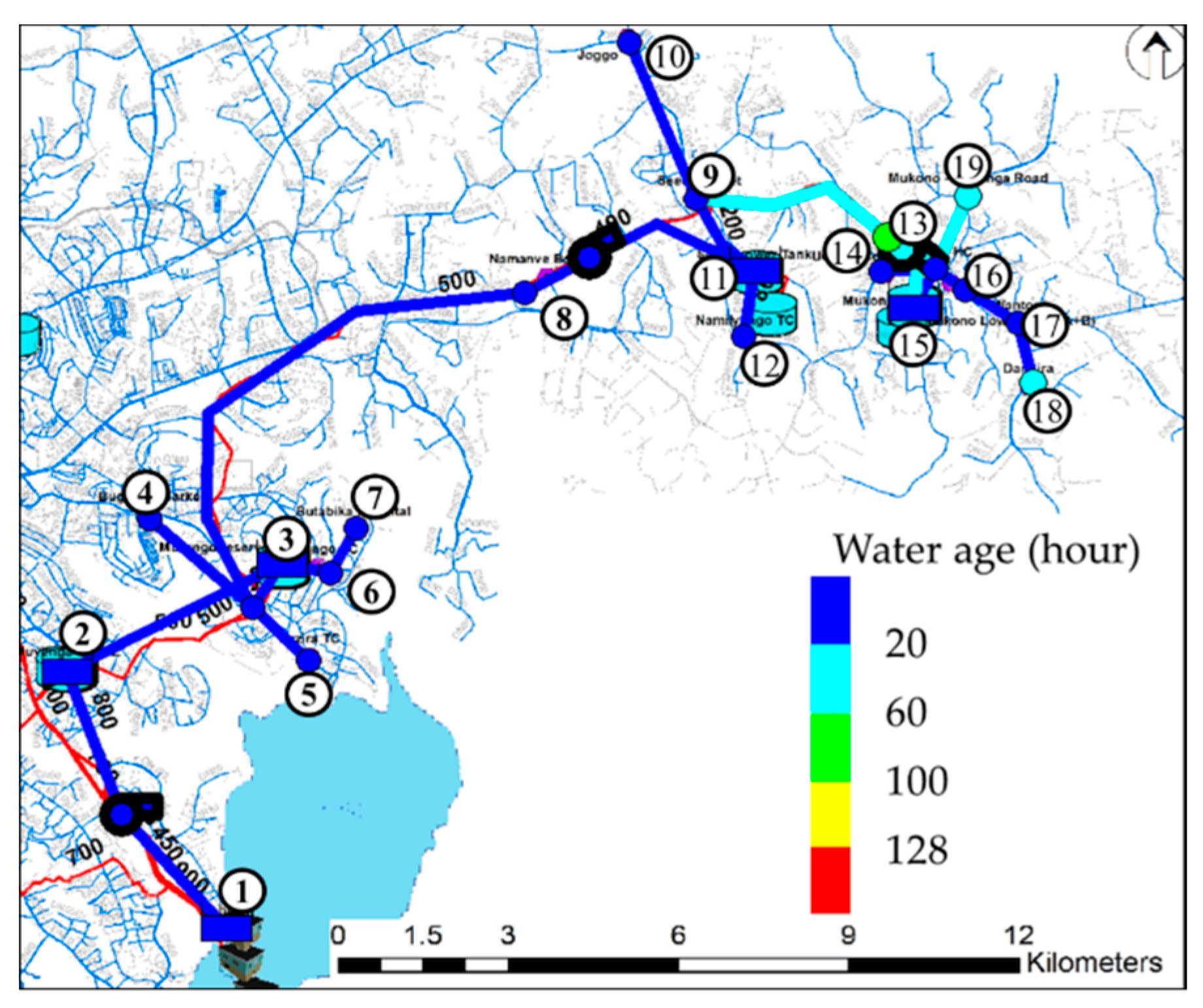
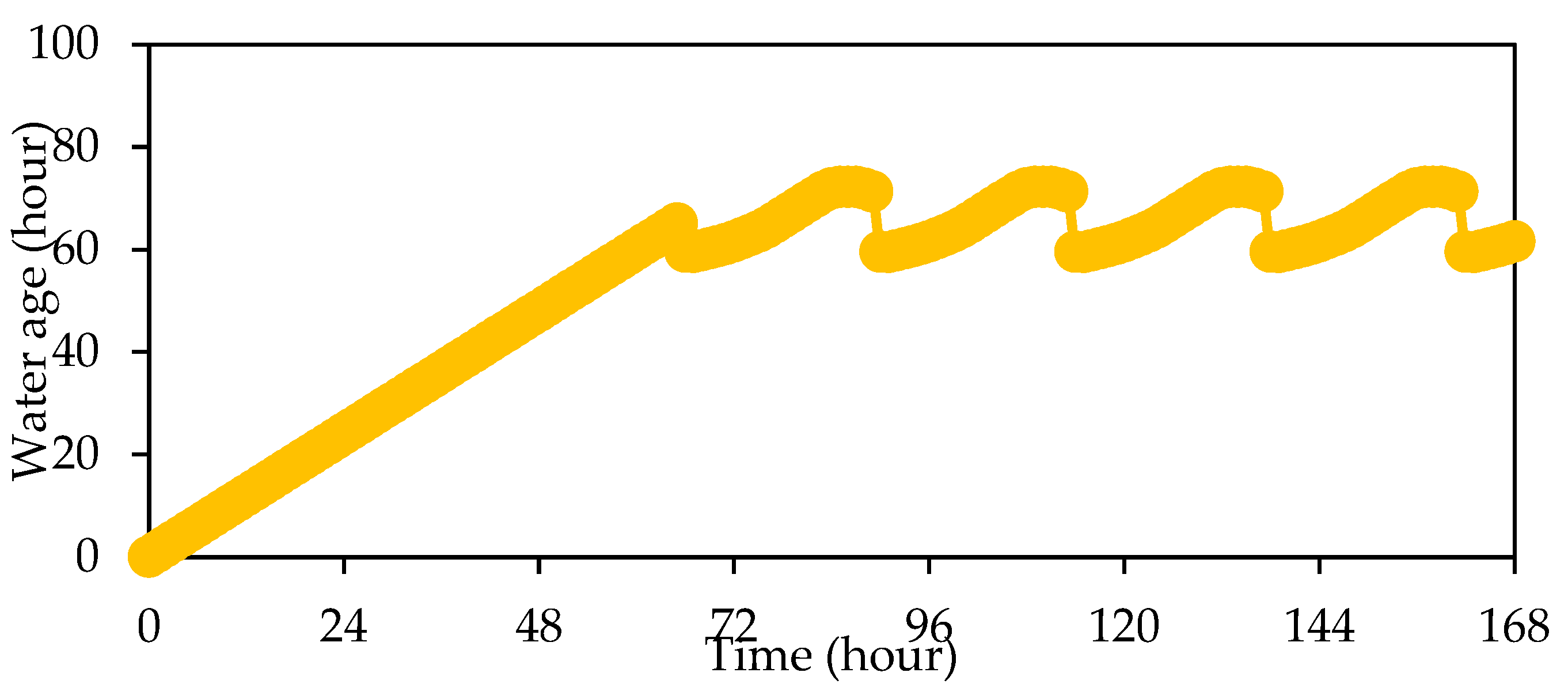
The water age at most sample locations was estimated to be less than 20 h; the water age at Mukono Health Centre was 72.3 h (Figure 4 and Figure 5), which is the highest value in this system, but is also well within the standard limit [32]. Seeta market, Namilyango TC (Trading Centre) and UCU (Uganda Christian University) Mukono (i.e., nodes numbered nine, 12 and 14 respectively) did not meet the minimum pressure head requirements of 17 psi at all times [8] (see Figure 6). At low pressures in the pipe, such as in UCU Mukono and Namilyango TC, contaminants could enter from the outside of the pipe.

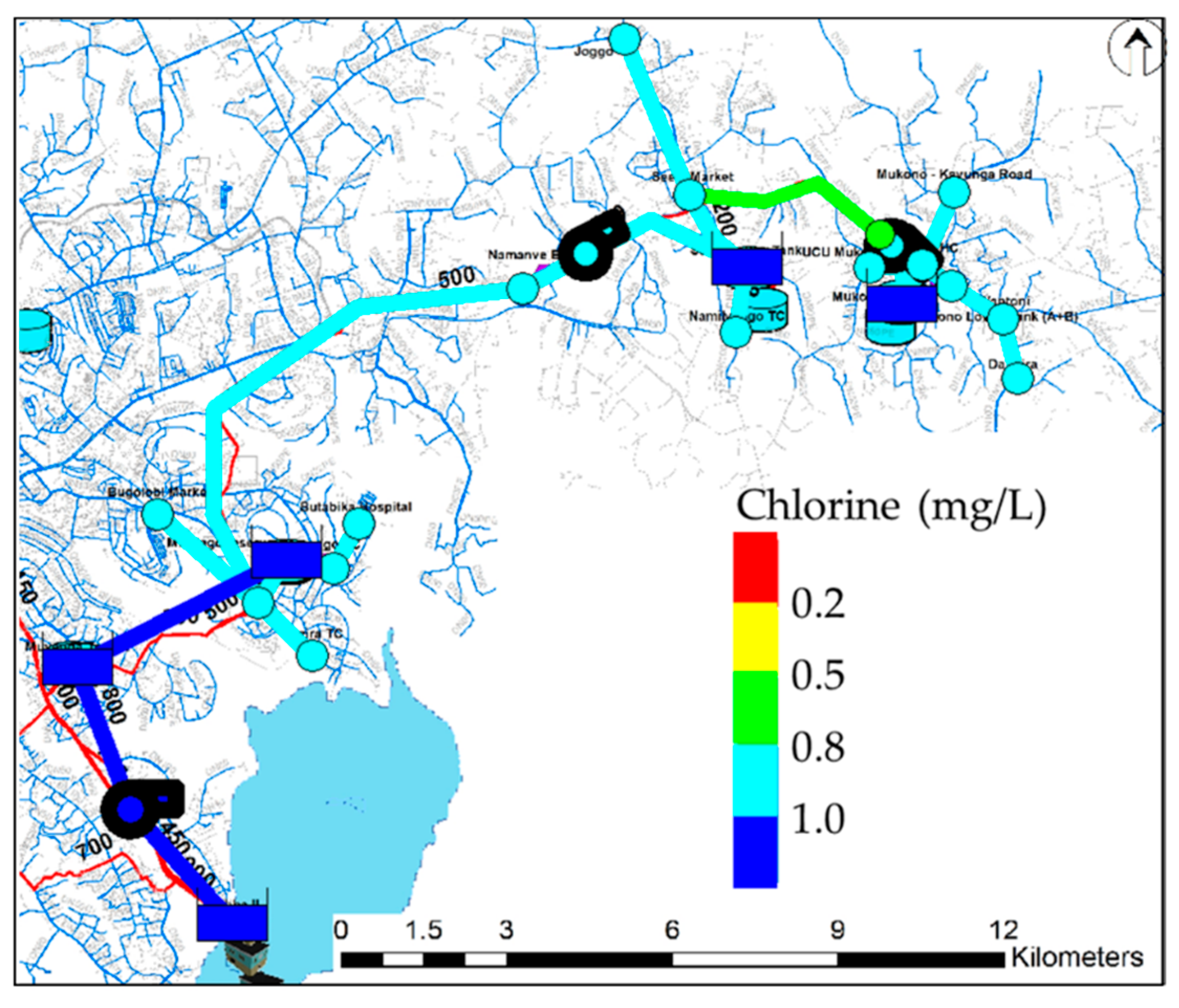
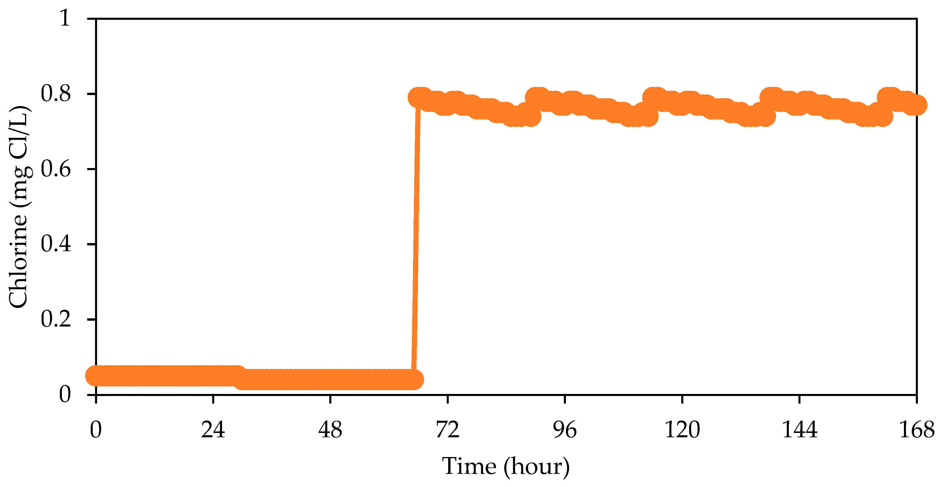
Chlorine, E. coli and COD did not meet their respective standards at many locations. Using EPANET simulations, it was found that it is possible to maintain the free chlorine in the entire system above 0.7 mg/L at all times by adding chlorine, so that its concentration in the service tanks becomes sufficiently high (1.0 mg/L or more, see Figure 7 and Figure 8). Since COD was below standard values at the exit of the water treatment plant, there is the possibility that organic matter entered from outside of the pipes due to low pressure, causing the increased COD at the sampling points, or the detachment of biofilm from pipe walls when hydraulic regimes/pressures change abruptly in the charging and discharging of pipes. If intrusion is a main culprit in COD increases, it is necessary to replace leaky pipes and joints that leak and improve operations that exasperate pipe damage and assess the impact using monitoring (e.g., COD and residual free chlorine). Free chlorine is sensitive to contaminants and its degradation can be used as an indicator of intrusion [38]. UCU Mukono and Namilyango TC, where pressure was low, did not meet free chlorine standards. Moreover, even at locations where minimum pressure standards were met, free chlorine levels did not meet the WHO standard. When comparing leaky sites and residual free chlorine along the network, we found that residual chlorine decreased after passing through Muyenga Tank E, where there are the most leaks reported (Figure 9). Similarly, cases of E. coli were mostly detected after Muyenga tank E. Therefore, intrusion from outside the pipes can be considered as probable cause. From these results, aging pipes are considered a main cause of water quality degradation in Mukono town. It has previously been reported that the large leakage levels, especially in the centre of Kampala as shown in Figure 9, are attributed to high rates of water theft, illegal connections, bursts and leakages [15,39]. Therefore, future work should explore the same parameters in the whole system, including a dense network of sampling in Kampala to get a better picture of risks associated to intrusion. Interventions in asset replacement can also be targeted to improve residual disinfection (e.g., plastic pipes, where free chlorine is more effective in preventing regrowth than in iron pipes [15]).

Although intrusion is our main suspect, it has also long been known that coliform regrowth (including faecal coliforms) is associated with biofilm regrowth in distribution systems [40,41]. High levels of coliform can be detected as a result of biofilm, even if very low levels are detected in effluent from the treatment plant. Since the residual chlorine levels of our case study were low anyway, it is possible that biofilms could play a part in bacterial regrowth. However, there were no known hydraulic disturbances and transients during the sampling campaign that imply the significant dislocation of biofilm and the very high levels of E. coli detected. Future work should consider the analysis of biofilm through grab sampling and fire hydrant experiments at a denser network of locations, taking into account the different pipe materials and ages. For example, heterotrophic plate counts (HPC) could be used as an indicator for the expanding of biofilms [21].

Although boosting the network with residual chlorine as a disinfectant is widely used, as proposed in our intervention, there are potential concerns that have to be considered in its use in addition to the capacity of residual chlorine to inactivate pathogens that gain entry to the network. Firstly, elevated levels of residual chlorine are associated with the unacceptable taste and odour of the drinking water for customers. However, our suggested intervention results in free chlorine levels were well below 1mg/L in the system, which is generally a range with no felt odour [42]. The case detection levels also vary widely between people, and can be based on the repeated experience of the taste [25]. Moreover, even if the dose needed to be high enough to result in a felt odour, it can be argued that safe water for the people (i.e., securing public and individual health) is more important than odour or taste. On the other hand, it is usually a low level of disinfectant that results in the development of discolouration, bad tastes and odours produced by biofilm. If such a case of felt odour is a concern in parts of the network, the utility should effectively communicate this to users for acceptance.

Another alternative is the use of chloramines instead of free chlorine as a residual disinfectant. This has been shown to perform better in the stability of residual concentrations throughout the distribution system, lower trihalomethane (THM) concentrations, better control of coliforms and heterotrophic plate count (HPC) bacteria [42]. It is also reported that chloramines result in less detectable taste and odour at much higher concentrations compared to free chlorine [25]. Although beyond the scope of this manuscript, the boost chlorination could also be optimised spatially and in time so that no part of the network has very high levels of residual chlorine. For example, common target concentrations for free chlorine in Europe are ~0.3 mg/L at the tap [25].

4. Conclusions

In this study, the water quality in the Kampala water distribution system was assessed from Ggaba II to Mukono town via Kampala and solutions were proposed to safeguard water quality. Using experimental data and EPANET modelling, boosting chlorine at tanks was proposed so that free chlorine concentration is at least 0.7 mg/L at all locations, to maintain residual disinfection and prevent contamination by E. coli and other biohazards. It is, therefore, possible to decrease intrusion in the network and increase the safety of water provided to consumers in Mukono town through a combination of water quality monitoring and booster disinfectant addition. Moreover, by showing a potential correlation between the water quality degradation and location of leaky pipes and low pressures, it was also recommended that preferentially upgrading leaky and damaged pipes should be done.

A further action for research would be to test the proposed intervention within the real distribution system in order to demonstrate its efficacy practically. Moreover, water quality data, which is collected continuously or through repetitive grab sampling, is needed to characterise disinfectant residual contaminations and indicator bacteria concentrations throughout the supply cycle, including during first flush [43]. As such, the approach can be applied in other similar systems using intermittent water supply to improve the water quality while the system transitions to continuous supply over many years. In future, inline disinfectant addition locations could also be optimised for a more uniform chlorine distribution [44,45].

References

- Charalambous, B.; Liemberger, R. Dealing with the Complex Interrelation of Intermittent Supply and Water Losses; International Water Association: London, UK, 2017; Available online: https://www.iwapublishing.com/books/9781780407067/dealing-complex-interrelation-intermittent-supply-and-water-losses (accessed on 12 January 2019).
- Van den Berg, C.; Danilenko, A. The IBNET Water Supply and Sanitation Performance Blue Book; The World Bank: Washington, DC, USA, 2011; Available online: http://documents.worldbank.org/curated/en/420251468325154730/The-IBNET-water-supply-and-sanitation-performance-blue-book (accessed on 22 February 2019).
- World Health Organization; UNICEF. Global Water Supply and Sanitation Assessment 2000 Report; World Health Organization: Geneva, Switzerland; UNICEF: New York, NY, USA, 2000; Available online: https://www.who.int/water_sanitation_health/monitoring/jmp2000.pdf (accessed on 12 January 2019).
- Government of Uganda Ministry of Water and Environment. Water and Sanitation Sector Performance Report 2006; Government of Uganda: Kampala, Uganda, 2006. Available online: https://docs.google.com/file/d/0BwhPKU71ZwQDSDc3eTdXMlpLV1U/edit (accessed on 22 June 2019).
- Intermittent Water Supply—A Paradigm Shift is Imperative. Available online: https://iwa-network.org/intermittent-water-supply-a-paradigm-shift-is-imperative/ (accessed on 25 June 2019).
- Vairavamoorthy, K.; Gorantiwar, S.D.; Mohan, S. Intermittent water supply under water scarcity situations. Water Int. 2007, 32, 121–132. [Google Scholar] [CrossRef]
- Barwick, R.S.; Uzicanin, A.; Lareau, S.; Malakmadze, N.; Imnadze, P.; Iosava, M.; Ninashvili, N.; Wilson, M.; Hightower, A.W.; Johnston, S.; et al. Outbreak of Amebiasis in Tbilisi, republic of Georgia, 1998. Am. Trop. Med. Hyg. 2002, 67, 623–631. [Google Scholar] [CrossRef] [Green Version]
- Kumpel, E.; Nelson, K.L. Mechanisms affecting water quality in an intermittent piped water supply. Environ. Sci. Technol. 2014, 48, 2766–2775. [Google Scholar] [CrossRef] [PubMed]
- Mutikanga, H.E.; Sharma, S.K.; Vairavamoorthy, K. Assessment of apparent losses in urban water systems. Water Environ. J. 2011, 25, 327–335. [Google Scholar] [CrossRef]
- Haward, G.; Pedley, S.; Tibatemwa, S. Quantitative microbial risk assessment to estimate health risks attributable to water supply: Can the technique be applied in developing countries with limited data? J. Water Health 2006, 4, 49–65. [Google Scholar] [CrossRef]
- IWA Connect. Available online: https://iwa-connect.org/group/intermittent-water-supply-iws/about?view=public (accessed on 26 June 2019).
- Klingel, P.; Nestmann, F. From intermittent to continuous water distribution: A proposed conceptual approach and a case study of Béni Abbès (Algeria). Urban Water J. 2014, 11, 240–251. [Google Scholar] [CrossRef]
- National Planning Authority (NPA), Government of Uganda. Uganda Vision 2040; NPA: Kampala, Uganda, 2013. Available online: https://www.greengrowthknowledge.org/sites/default/files/downloads/policy-database/UGANDA%29%20Vision%202040.pdf (accessed on 8 January 2019).
- The Republic of Uganda, Ministry of Water and Environment. Framework and Guidelines for Water Source Protection Volume 2: Guidelines for Protecting Water Sources for Piped Water Supply Systems; The Republic of Uganda Ministry of Water and Environment: Kampala, Uganda, 2013. Available online: https://www.mwe.go.ug/sites/default/files/library/Vol.%202%20-%20Guidelines%20for%20Protecting%20Piped%20Water%20Sources%20-%20FINAL.pdf (accessed on 10 January 2019).
- Ecuru, J.; Okumu, O.J.; Okurut, O.T. Monitoring residual chlorine decay and coliform contamination in water distribution network of Kampala, Uganda. Afr. J. Online 2011, 15, 167–173. [Google Scholar] [CrossRef]
- Rossman, L. EPANET 2 User’s Manual; Risk Reduction Engineering Laboratory, U.S. Environmental Protection Agency: Cincinnati, OH, USA, 2000.
- Uganda Bureau of Statistics Population and Censuses, Population Projections 2018. Available online: https://www.ubos.org/explore-statistics/20/ (accessed on 30 June 2019).
- The Republic of Uganda Ministry of water and environment. Water Supply Design Manual Second Edition; The Republic of Uganda Ministry of Water and Environment: Kampala, Uganda, 2013. Available online: https://www.mwe.go.ug/sites/default/files/library/Water%20Supply%20Design%20Manual%20v.v1.1.pdf (accessed on 12 January 2019).
- Kalibbala, H.M.; Nalubega, M.; Wahlberg, O.; Hultman, B. Performance Evaluation of Drinking Water Treatment Plants in Kampala—Case of Ggaba II. In Proceedings of the 32nd WEDC International Conference, Colombo, Sri Lanka, 13–17 November 2006; pp. 373–376. [Google Scholar]
- Environmental Protection Agency. Quick Guide to Drinking Water Sample Collection; Environmental Protection Agency: Washington, DC, USA, 2016. Available online: https://www.epa.gov/sites/production/files/2015-11/documents/drinking_water_sample_collection.pdf (accessed on 22 February 2019).
- Blokker, M.; Furnass, W.; Machell, J.; Mounce, S.; Schaap, P.G.; Boxall, J. Boxall. Relating Water Quality and age in drinking water distribution systems using self-organising maps. Environments 2016, 3, 10. [Google Scholar] [CrossRef] [Green Version]
- Minnesota Pollution Control Agency. Turbidity: Description, Impact on Water Quality, Sources, Measures—A General Overview; Minnesota Pollution Control Agency: St Paul, MN, USA, 2008. Available online: https://www.pca.state.mn.us/sites/default/files/wq-iw3-21.pdf (accessed on 20 February 2019).
- World Health Organization. pH in Drinking-Water Background Document for Development of WHO Guidelines for Drinking-Water Quality; World Health Organization: Geneva, Switzerland, 2014. [Google Scholar]
- Cotruvo, J.A. 2017 WHO guidelines for drinking water quality: First addendum to the fourth edition. J. Am. Water Works Assoc. 2017, 109, 44–51. [Google Scholar] [CrossRef] [Green Version]
- Ainsworth, R. Safe Piped Water: Managing Microbial Water Quality in Piped Distribution Systems; World Health Organization: Geneva, Switzerland, 2004; Available online: https://apps.who.int/iris/handle/10665/42785 (accessed on 12 January 2019).
- Geldreich, E. Microbial Quality of Water Supply in Distribution Systems; CRC Lewis Publishers: Boca Raton, FL, USA, 1996. [Google Scholar]
- William, D.H.; Robert, S.S.; Elston, S.; Sharon, C.M.; Marjorie, G.B.; Barbara, G.S.; Susan, N.P. Intestinal effects of sulphate in drinking water on normal human subjects. Dig. Dis. Sci. 1997, 42, 1055–1061. [Google Scholar] [CrossRef]
- Prest, E.I.; Hammes, F.; van Loosdrecht, M.C.; Vrouwenvelder, J.S. Biological stability of drinking water: Controlling factors, methods, and challenges. Front. Microbiol. 2016, 7, 45. [Google Scholar] [CrossRef] [PubMed]
- World Health Organization. Ammonia in drinking-Water Background Document for Development of WHO Guidelines for Drinking-Water Quality; World Health Organization: Geneva, Switzerland, 2001; Available online: https://www.who.int/water_sanitation_health/water-quality/guidelines/chemicals/ammonia.pdf?ua=1 (accessed on 12 January 2019).
- World Health Organization. Nitrate and Nitrite in Drinking-Water Background Document for Development of WHO Guidelines for Drinking-Water Quality; World Health Organization: Geneva, Switzerland, 2016; Available online: https://apps.who.int/iris/handle/10665/75380 (accessed on 12 January 2019).
- Ministry of the Environment Government of Japan. Available online: https://www.env.go.jp/en/index.html (accessed on 12 January 2019).
- Wang, H.; Masters, S.; Hong, Y.; Stallings, J.; Falkinham, J.O., III; Edwards, M.A.; Pruden, A. Effect of disinfectant, water age, and pipe material on occurrence and persistence of Legionella, mycobacteria, Pseudomonas aeruginosa, and two amoebas. Environ. Sci. Technol. 2012, 46, 11566–11574. [Google Scholar] [CrossRef] [PubMed]
- Tadeusz, J. Swierzawski. Piping Handbook 7th Edition, Flow and fluids Chapter B8; MCGRAW-HILL: New York, NY, USA, 2000; Available online: https://engineeringdocu.files.wordpress.com/2011/12/piping-handbook.pdf (accessed on 23 February 2019).
- Ozdemir, O.N.; Ucak, A. Simulation of chlorine decay in drinking-water distribution systems. J. Environ. Eng. 2002, 128, 31–39. [Google Scholar] [CrossRef]
- Vieira, P.; Coelho, S.T.; Loureiro, D. Accounting for the influence of initial chlorine concentration, TOC, iron and temperature when modeling chlorine decay in water supply. J. Water Supply Res. Technol. AQUA 2004, 53, 453–467. [Google Scholar] [CrossRef]
- Al-Jasser, A.O. Chlorine Decay in Drinking-Water Transmission and distribution systems: Pipe service age effect. Water Res. 2007, 41, 387–396. [Google Scholar] [CrossRef]
- Housing and Building National Research Centre. Egyptian Code for Design and Implementation of Pipeline Networks for Drinking Water and Sanitation, 10th ed.; Housing and Building National Research Centre: Cairo, Egypt, 2007. [Google Scholar]
- Helbling, D.E.; Van Briesen, J.M. Modeling residual chlorine response to a microbial contamination event in drinking water distribution systems. J. Environ. Eng. 2009, 135, 918–927. [Google Scholar] [CrossRef]
- The Republic of Uganda, Ministry of Water and Environment. Uganda Water and Environment Sector Performance Report 2017; The Republic of Uganda Ministry of Water and Environment: Kampala, Uganda, 2017. Available online: https://www.mwe.go.ug/sites/default/files/library/SPR%202017%20Final.pdf (accessed on 20 February 2020).
- LeChevallier, M.W.; Babcock, T.M.; Lee, R.G. Examination and characterization of distribution system biofilms. Appl. Environ. Microbiol. 1987, 53, 2714–2724. [Google Scholar] [CrossRef] [Green Version]
- Flemming, H.-C.; Percival, S.; Walker, J.T. Contamination potential of biofilms in water distribution systems. Water Sci. Technol. Water Supply 2002, 2, 271–280. [Google Scholar] [CrossRef]
- Norton, C.D.; LeChevallier, M.W. Chloramination: Its effect on distribution system water quality. Am. Water Works Assoc. J. 1997, 89, 66–77. [Google Scholar] [CrossRef]
- Kumpel, E.; Nelson, K.L. Intermittent water supply: Prevalence, practice, and microbial water quality. Environ. Sci. Technol. 2015, 50, 542–553. [Google Scholar] [CrossRef]
- Xin, K.; Zhou, X.; Qian, H.; Yan, H.; Tao, T. Chlorine-age based booster chlorination optimization in water distribution network considering the uncertainty of residuals. Water Supply 2018, 19, 796–807. [Google Scholar] [CrossRef]
- Tryby, M.E.; Boccelli, D.L.; Uber, J.G.; Rossman, L.A. Facility location model for booster disinfection of water supply networks. J. Water Resourc. Plan. Manag. 2002, 128, 322–333. [Google Scholar] [CrossRef]
Figure 1.
Kampala water distribution systems and pipelines from Ggaba II to Mukono town. The names of the numbered sites are shown in Table 1.
Figure 2.
Typical weekday consumption patterns (normal households aggregated, township taps, schools and total of the three patterns) in Kampala water distribution systems [18].
Figure 3.
Free chlorine (a), E. coli (b) and COD (c) measurements from the Kampala water distribution system. The place numbers are as shown in Table 1 (n = 2). The error bars show the standard deviation of duplicate samples.
Figure 4.
Water age in Kampala water distribution system. The overlaid colour of the node indicates water age after 130 h when the chlorine dynamics had stabilised with diurnal variations. The names of the numbered sites are shown in Table 1.
Figure 5.
Water age at Mukono Health Centre (No. 13), the highest value in the system.
Figure 6.
Kampala water distribution system and pipeline from Ggaba II to Mukono. The name of the numbered sites is shown in Table 1. The overlaid colour of nodes indicates water pressure.
Figure 7.
Kampala water distribution system and pipeline from Ggaba II to Mukono. The name of the numbered sites is shown on the Table 1. The overlaid colour of pipelines indicates free chlorine levels after 24 h adding chlorine at reservoirs.
Figure 8.
Free chlorine value at Mukono Health Centre (No. 13), lowest value for the system.
Figure 9.
Kampala water distribution system and pipeline from Ggaba II to Mukono with leak occurrences (green circles) overlaid with E. coli measurements (a) and COD measurements (b). The name of the numbered sites is shown on the Table 1.