
Calculation of Multiple Critical Depths in Open Channels Using an Adaptive Cubic Polynomials Algorithm

Department of Civil Engineering, University of Thessaly, Pedion Areos, 38334 Volos, Greece
*
Author to whom correspondence should be addressed.
Water 2020, 12(3), 799; https://doi.org/10.3390/w12030799
Submission received: 28 December 2019
/
Revised: 15 February 2020
/
Accepted: 28 February 2020
/
Published: 13 March 2020
(This article belongs to the Special Issue Insights on the Water–Energy–Food Nexus)
Abstract
:A method for the calculation of multiple critical depths in compound and natural channels, using an adaptive cubic polynomials algorithm (ACPA), is presented in this paper. The algorithm is based on the approximation of the specific energy with multiple cubic polynomials. The roots of these polynomials’ derivatives are determined to calculate all local minima and maxima. These extremities yield the critical depths. Furthermore, the Froude number can be calculated at any elevation by applying a simple formula after calculating the derivative of the corresponding polynomial, which contains the given elevation. The algorithm developed was tested on various compound and natural channels. Its results were then compared with the results provided by the HEC-RAS (Hydrologic Engineering Center – River Analysis System) computer program, proving that in some cases ACPA results were more accurate than those of HEC-RAS. This has to do with the fact that HEC-RAS algorithm determines a single critical depth and is better fitted to simple prismatic channels. On the other hand, the ACPA algorithm is able to calculate all critical depths of a natural or compound channel, providing thus more accurate results.
1. Introduction
A flow in an open channel may be either deep with low velocity or shallow with high velocity. In the first case, the flow is subcritical while in the latter it is supercritical. In the special case where the flow is neither subcritical nor supercritical, it is critical. The depth where critical flow occurs (critical depth) generally depends on the geometry of the channel and the discharge value.
The actual depth and velocity of the flow for a specific discharge depends on the friction coefficient and the slope of the channel’s bed and can be directly calculated via Manning’s equation:
where: Q (m3/s) is the discharge; n (s/m1/3) is the Manning’s coefficient; A (m2) is the cross-sectional area of flow (which depends on the flow depth); R=A/p (m) is the hydraulic radius (m), where P (m) is the wetted perimeter (which also depends on the flow depth); and finally S is the slope of the channel’s bed.
Calculation of the critical depth is very important, as an open channel should be protected from erosive conditions caused by unstable critical flow or high velocity supercritical flow. Thus, appropriate fine tuning (adjustment) of the channel’s geometrical parameters should take place during the channel’s designing phase to avoid these kinds of flows.
Froude number gives an indication of the flow regime. If the Froude’s number is lower than 1, then the flow is subcritical, while if it is higher than 1, then the flow is supercritical. When the Froude’s number equals 1 then the flow is critical. Froude number is related to the slope of the specific energy curve based on Equation (2) [1,2,3]:
where: H is the specific energy [4]; and y is the flow depth.
Therefore, when the slope of the specific energy curve is positive, the flow is subcritical, while negative slope indicates supercritical flow. Finally, when the slope is zero, the flow is critical [5].
The specific energy in simple prismatic channels (i.e. rectangular, trapezoidal) for a given discharge gets its minimum value only when the flow depth gets a specific value [6]. Thus, there is only one critical depth in such channels for every discharge value. It has been proven, both in the lab and through numerical modelling, that in open channels with overbanks (compound channels), more than one critical depth may occur for a given discharge [2,7,8]. The specific energy at these depths has local minima, but may also have maxima as well, as Chaudhry and Bhallamudi showed [9]. Although Blalock and Sturm [2] defined a Froude number for compound channels, which correctly locates the exact positions where the minima and maxima of the specific energy occurs, they didn’t provide a solid procedure to calculate the critical depths related.
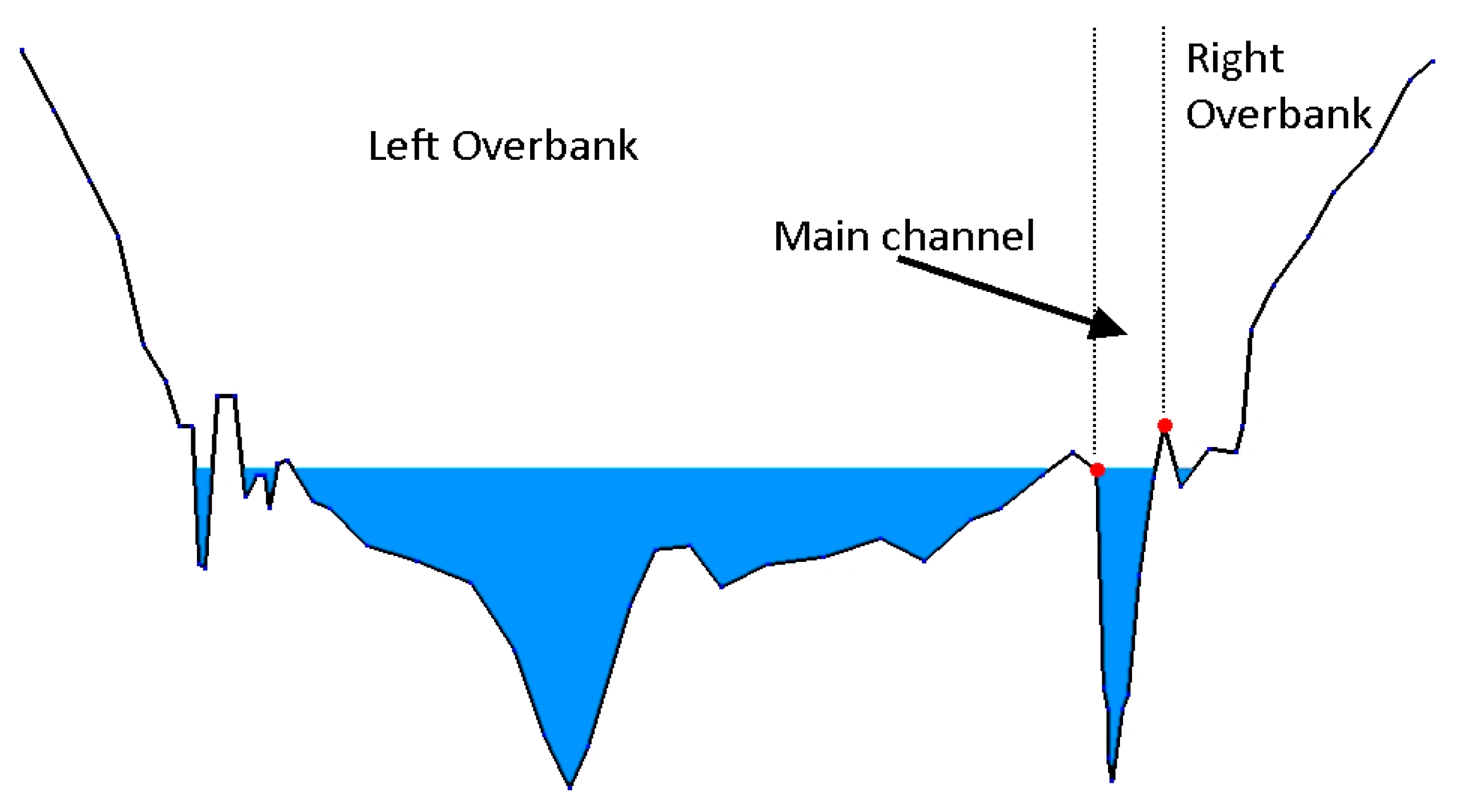
Although prismatic and compound channels are usually artificial ones, it is essential to deal with natural open channels that are irregularly shaped by the ground, when studying river flows or floods. The shape of such channels (Natural Channels) can be determined by either elevation maps or simply extracted by Digital Elevation Models (D.E.M.) [10,11,12] together with the drainage networks and the associated hydrological characteristics [13,14,15,16]. These channels are commonly described by several sections (Natural Sections) vertical to the flow path, taken at various intervals. Each section consists of three regions, the main channel and the two overbanks. As overbank might be either artificial or natural, covered or not with vegetation, it might have its own friction coefficient (Figure 1). To describe the properties and characteristics of this type of sections, the flow calculation software HEC-RAS (Hydrologic Engineering Center-River Analysis System) [17] is usually used [18].
2. The Proposed Approach
In order to pinpoint the critical depths of a natural section, specific energy needs to be calculated:
where: α is the kinetic energy correction factor; V is the mean flow velocity; and Q is the discharge.
The cross-sectional area of flow A is a strictly monotonically increasing function of the flow depth and can be calculated by the section’s geometry. The kinetic energy correction factor α on the other hand, depends on the cross-sectional areas and conveyances of each region and the total cross-sectional area and total conveyance as well [6]:
where: Alob, Ach and Arob are the cross-sectional areas of the left overbank, main channel and right overbank respectively; Klob, Kch and Krob are the conveyances of the left overbank, main channel and right overbank respectively; and K is the total conveyance (i.e. the sum of the partial conveyances). The conveyances of the left overbank, main channel and right overbank along with the total conveyance can also be easily calculated (Equations (5)–(8)).
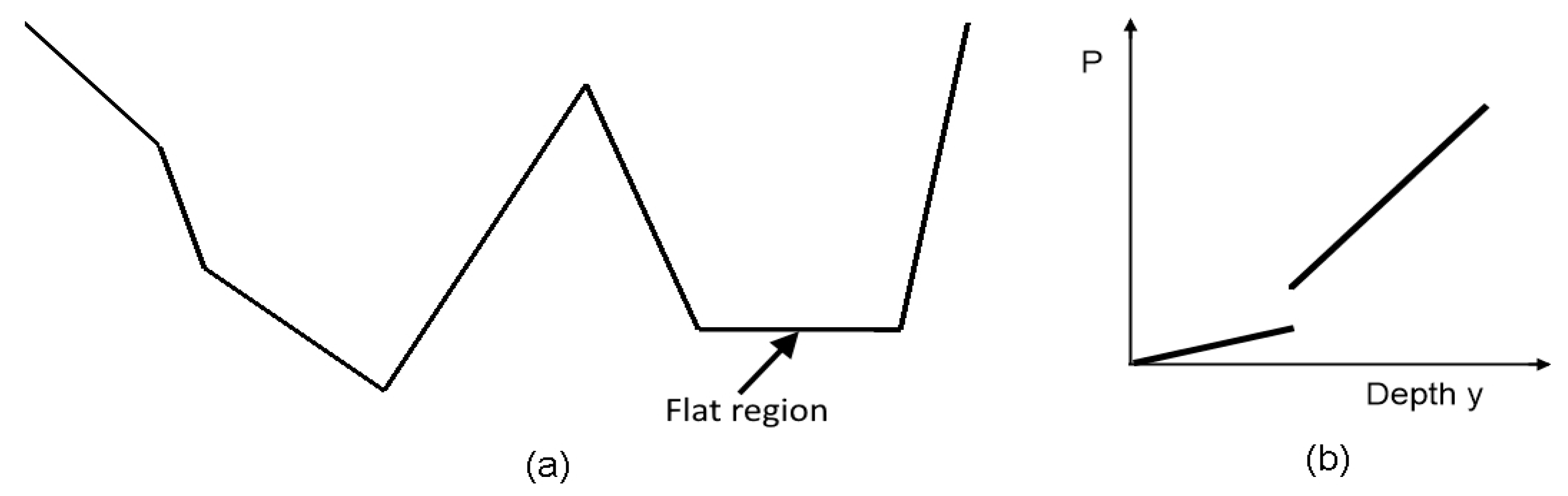
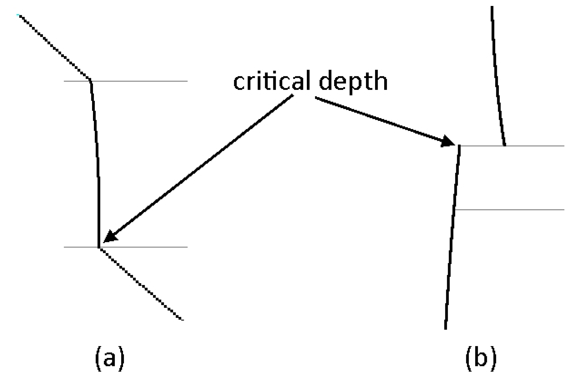
The hydraulic radius R is a non-monotonic function of the flow depth and may also have discontinuities when the section contains flat regions, since the wetted perimeter in such cases is discontinuous (Figure 2a,b). Consequently, the respective conveyance will also be non-monotonic with possible discontinuities.
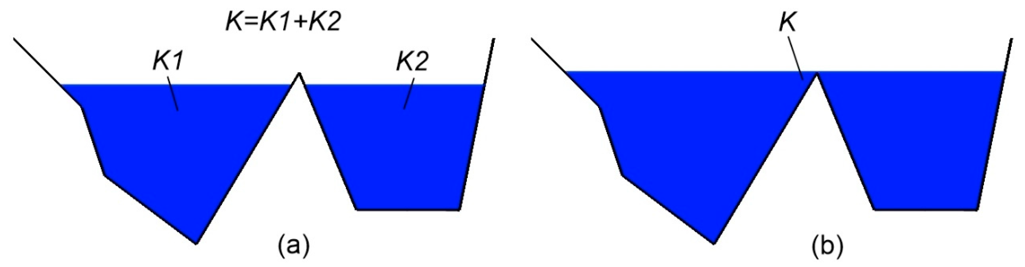
Another issue is that for certain section shapes and depths, the flow may be divided in two or more parallel flows (Figure 3a). When this happens, the conveyance for each parallel flow is being separately calculated, while the total conveyance is the sum of all these individual conveyances. Eventually after a certain depth, the divided flows join up into a single one (Figure 3b). At this point, the conveyance is being calculated as a whole, leading again to a discontinuity.
For all these reasons, the kinetic energy correction factor a is non-monotonic and may have discontinuities. The same also stands for the specific energy H which apart from the discontinuities may have multiple minima or maxima and thus, result in multiple critical depths.
In this study, an approximation of the specific energy using multiple cubic polynomial functions is being proposed. The approximation of hydraulic or hydrological parameters using polynomials is a widely used technique, which allows the analytical calculations of these parameters. As polynomial functions can be easily differentiated, it is therefore very easy to calculate the curve’s slope and from there, applying equation 2, the Froude’s number.
Furthermore, since the polynomials are cubic, their derivatives are quadratic polynomials. The roots of quadratic polynomials can be easily extracted and thus the depths of the local minima or maxima can be easily determined. These are of course the critical depths.
As mentioned before, the specific energy might be a discontinuous function. The first step is to determine the exact points of its possible discontinuities. The section’s geometry is defined by a set of X-Y points, where X is the distance from the leftmost side of the section, as seen from upstream to downstream, while Y is the elevation. Between any two successive Y elevations (Figure 4a), the section increases by multiple trapezoidal subsections (Figure 4b). This means that the area is increased by the sum of the areas of all these trapezoidal subsections and the wetted perimeter is increased by the sum of the wetted perimeters of the same trapezoidal sections (Figure 4c). The area of a single trapezium is a quadratic polynomial of the depth, while its wetted perimeter is a linear polynomial of the depth. The sum of quadratic polynomials is a quadratic polynomial and likewise the sum of linear polynomials is a linear polynomial too. Consequently, between two successive elevations, the area and wetted perimeter of the section can be easily calculated (Equations (9) and (10)).
where: Aprev and Pprev are the area and wetted perimeter respectively, just before the lower of the two elevations; α1, b1, c1A are the coefficients of the quadratic polynomial for the calculation of the area; α2, b2A are the coefficients of the linear polynomial for the calculation of the wetted perimeter; and y is the depth. Merging the constant terms c1A and b2A with Aprev and Pprev respectively, yields:
The hydraulic radius R is a quotient of two polynomials, hence it is a rational function and as such it is continuous and differentiable. The conveyances Klob, Kch and Krob are power functions of Rlob, Rch and Rrob (Equations (5)–(7)) respectively, therefore they are continuous and differentiable too. The same stands also for the total conveyance K (Equation (8)). The kinetic energy correction factor α (Equation (4)) in turn, consists of continuous and differentiable terms and thus it is continuous and differentiable as well. The same stands for the specific energy too. Presumably, it can be concluded that between any two successive elevations of the section, the specific energy is continuous and differentiable and therefore can be approximated by a suitable interpolation function. By selecting multiple functions, one for each elevation interval, the whole specific energy curve can be approximated.
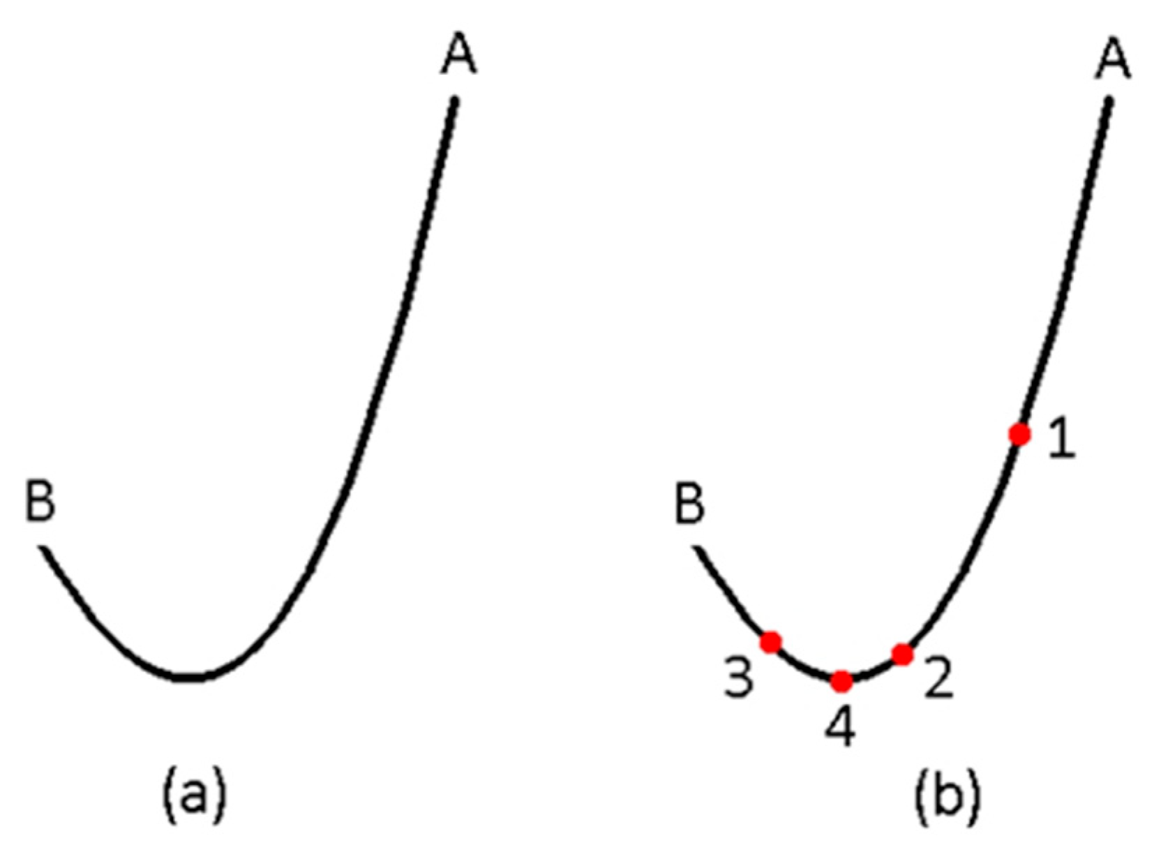
As mentioned before, the selection of cubic polynomials for the interpolation offers two important advantages, resulting from the fact that they can be analytically differentiated: a) the derivative from Equation (2) yields the Froude number; and b) if this derivative is set to zero, its roots are the critical depths. Furthermore, cubic polynomials provide adequate flexibility to interpolate various shapes. In general, most of the times, the shape of the specific energy curve resembles quadratic polynomials and therefore it can be easily interpolated by cubic polynomials. Occasionally, its shape is flat on one end and highly curved on the other (Figure 5a). In such cases the result of the proposed approximation could be quite inaccurate.
The solution adopted in the current study was to subdivide the interval into two equal ones. Then, each interval is examined, whether it satisfies or not certain criteria of “flatness” (Figure 5a). If this condition is not satisfied, then the subdivision continues until the shape of the intervals formed meets the specified criteria. Figure 5b presents such a successive approach. The first subdivision takes place at point 1, forming an adequately “flat” segment A-1 and another segment 1-B which needs to be subdivided as it not flat enough. The second subdivision takes place at point 2, forming a “flat” segment 1-2 and in a not that flat segment 2-B which needs to be subdivided too. Subdivision at point 3, results in a “flat” segment 3-B and in the segment 2-3 which needs to be subdivided as it not flat enough. Finally, subdivision at point 4 results in the segments 2-4 and 4-3 which are both “flat”. This signals the end of the “subdividing” process.
All necessary subdivisions are being automatically done by the algorithm developed herein until all interpolated segments are adequately “flat”. Thus, the resulting cubic polynomials are considered adaptive and the algorithm is named adaptive cubic polynomials algorithm (ACPA).
3. Adaptive Cubic Polynomials Algorithm (ACPA)
Initially, all elevations of the section are sorted in increasing order and any duplicates are removed. This results in an array of n elevations y1, y2, …, yn and n-1 segments y1-y2, y2-y3, …, yn-1-yn. As proven above, the curve of the specific energy is continuous and differentiable in each one of these segments. Figure 6 presents an example, in which a part of the specific energy curve appears. The horizontal lines show the sorted elevations. At y10, y11 and y14, the curve is continuous but at y12 and y13 it is not. The discontinuities, as mentioned before, occur either due to flat parts of the section or due to parallel flows which join up, changing the way the conveyance K is calculated.
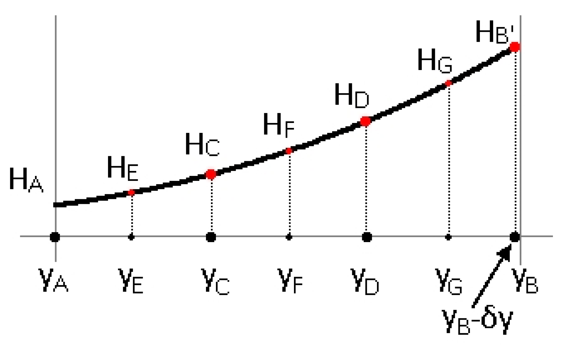
Then, for each segment between elevations yA and yB, the specific energy at four different elevations yA, yB’, yC and yD (Figure 7) can be easily calculated (Equations (13)–(15)).
where: δy is a small amount in the order of 1e-5. This is necessary because the discontinuities occur at y=yB, therefore, by decreasing y, continuity is guaranteed.
The four unknown coefficients α, b, c and d of the cubic polynomial can be calculated by solving the following linear system of equations:
At this point, the candidate cubic polynomial has been defined. The specific energy can now be calculated at any intermediate point through Equation (17).
Likewise, the first and second derivatives can also be directly calculated through the Equations (18) and (19)
The next task is to assess the accuracy of the approximation approach through a stepwise process which includes the three following checks:
- ✓
- Check 1 (convex concave): check whether there is an inflection point inside the segment or not. In other words, if the curve turns from convex to concave or vice versa. In that case, the segment must be subdivided. The second derivative at inflection points is zero. Therefore, it is adequate to calculate H’’ at both ends of the segment and check the signs. If they differ, then at some point inside the segment H’’ becomes zero and thus the segment must be subdivided.
- ✓
- Check 2 (curvature): check whether the slope of the curve changes significantly or not. In that case the segment must be subdivided. H’ is calculated at both ends yielding and . Then, the following three conditions are being checked:
- Condition 1: , where δ in this study was taken 0.5*
- Condition 2:
- Condition 3: , where ratiomin in this study was taken 0.4*
If condition 1 is true and either condition 2 or 3 is true, the segment must be subdivided. The values used for δ and ratiomin were determined with experiments. Several combinations were tried and the best results occurred for these values. - ✓
- Check 3 (fit): check whether the curve is fitted well or not. In the latter case it must be subdivided. H can be easily calculated at three additional intermediate elevations yE, yF, yG (Equations (20)–(22))
The calculation is analytically conducted resulting in HE, HF and HG. The values of the specific energy can be directly evaluated by the cubic polynomial at the same elevations (HpE, HpF and HpG). The calculated values are being compared in pairs:
where: tol is the tolerance, which in this study was 0.003m (3mm) for SI units or 0.01ft for English units.
If any of these conditions is true, then the segment is subdivided. At the end of this stepwise process, the whole curve has been approximated by the cubic polynomials. The critical depths can now be calculated. The first derivative of each polynomial is set to zero and its roots are determined:
Since it is a quadratic function, the roots can be easily calculated with the discriminant:
If the latter is negative, no roots exist. Otherwise, one or two roots are calculated:
Each root is checked whether it lies inside the segment or not. Roots lying outside the segment are discarded. The valid roots calculated are the critical depths.
The critical depths determined through the above stepwise procedure are not necessarily the only critical depths. As already mentioned, when the slope of the specific energy curve is positive, the flow is subcritical, while a negative slope indicates supercritical flow. Considering that the sign of the slope of the specific energy curve changes at the critical depth, elevations where the specific energy curve is not continuous or differentiable need be checked as well, as it might be an indication of a respective critical depth. More specifically, these elevations, as explained before, are actually the ending points of the previously defined segments (Figure 8). If the slope of the specific energy curve at the end of one segment has a different sign than the slope at the beginning of the next segment, this means that the flow changes regime from subcritical to supercritical or vice versa and thus the common elevation of the two segments must be of a critical depth.
In order to locate these critical depths, each segment (having the characteristics discussed before) should be in pairs, checked with its neighbor segment in order for their first derivatives to be calculated at their common elevation. If the derivatives are found to have opposite signs, then the common elevation is a critical depth. The number of critical depths found is always an odd number. This can be explained as follows: for shallow depths, flow is supercritical, so the first critical depth signifies the transition to subcritical flow. If another critical depth is found, it signifies the transition to supercritical flow. Therefore, every odd critical depth leads to subcritical and every even critical depth to supercritical flow. Since, for deep depths, the flow is subcritical, then the number of critical depths must be odd. Apart from the critical depths, the fact that the entire specific energy curve has been approximated using polynomials allows one to calculate the Froude number at any point. This is being done by calculating the first derivative of the corresponding polynomial at the given elevation, and then applying Equation (28), that resulted by combining Equations (2) and (18). Table 1 presents an outline of the ACPA algorithm.
4. Tests and Comparison
As mentioned in the previous sections, the calculation of the critical depths is based on the calculation of the specific energy. Considering this, an appropriate algorithm (referred to hereafter as Energy Calculation Algorithm—ECA) was developed in the current study and was properly adjusted to become compatible with HEC-RAS in order for their results to become comparable. ACPA and ECA need to be validated in order to ensure the reliability of the results. Four datasets where formed in order to be used during the validation process and tests and comparisons. More analytically:
Dataset 1 consists of 46 non symmetric trapezoidal sections with random bed width and random side slopes each. The depths are expressed in (m) and the discharges in (m3/s). Each section consists of a single channel without overbanks and a single random friction coefficient. The upstream discharge is 30m3/s at section 46 and remains constant for all sections.
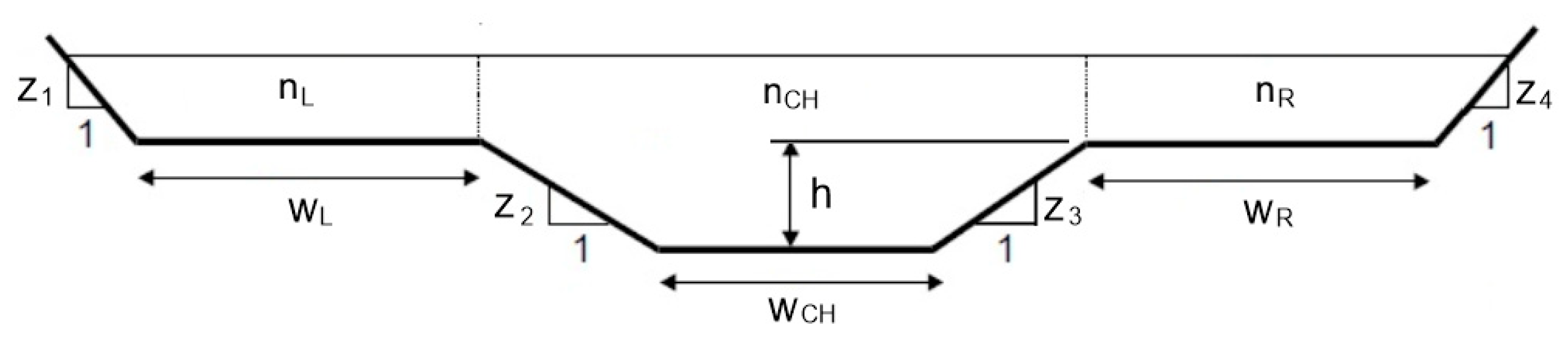
Dataset 2 consists of 164 non symmetric two stage trapezoidal compound sections (Figure 9). The depths are expressed in (m) and the discharges in (m3/s). Each section consists of a channel and two nonsymmetric overbanks with different friction coefficients. A great number of sections and discharges (more than 20 million) were examined and those presenting multiple critical depths were selected. The discharge at each section is set to the value specified by this procedure. One of the sections of Dataset 2 is the compound section presented in Figure 10. This section was used by Blalock and Sturm [2], Chaudhry and Bhallamudi [9] and other researchers. It consists of a rectangular channel with friction coefficient 0.013 and two symmetric overbanks with friction coefficient 0.0144.
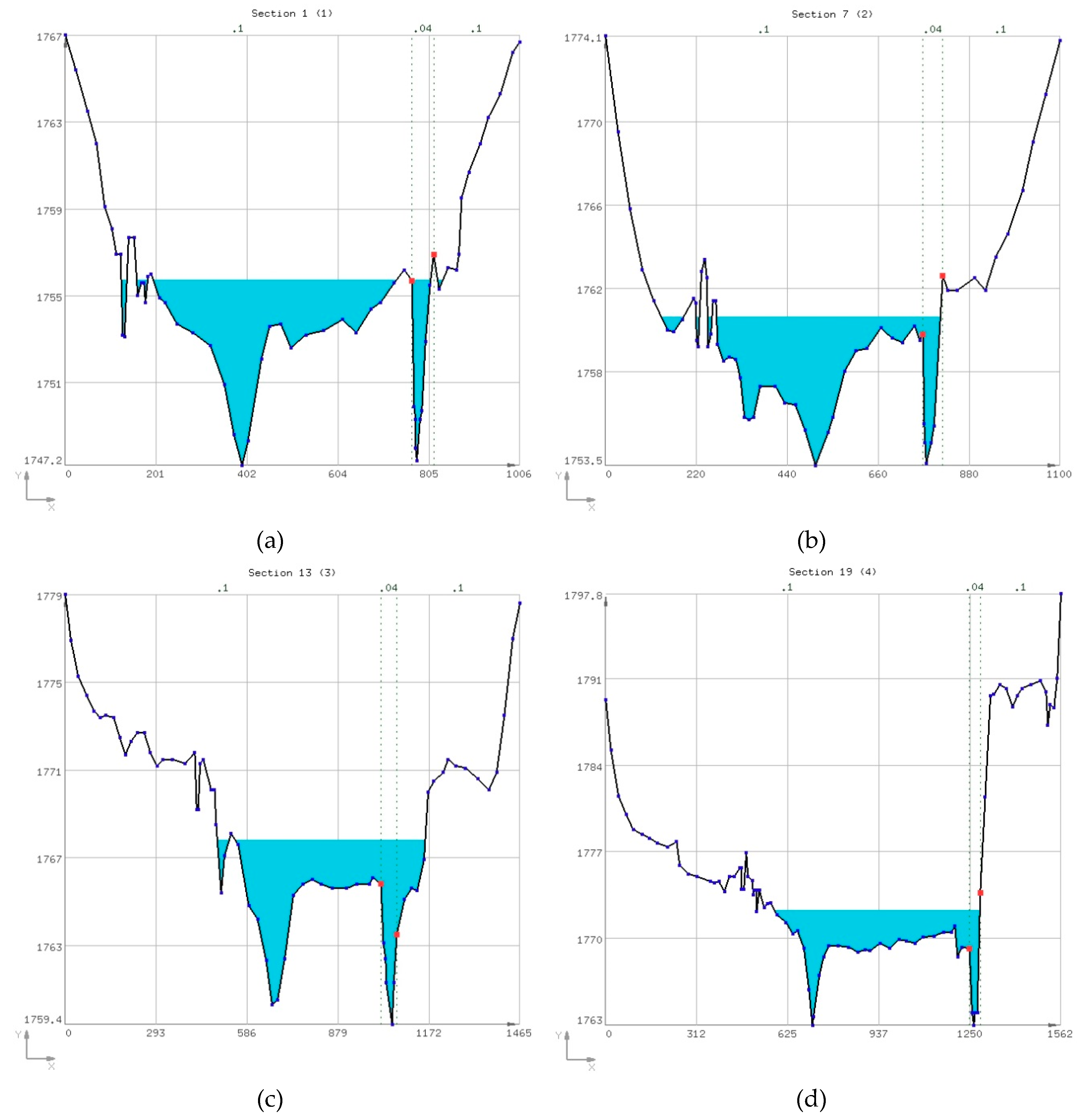
Dataset 3 is a well known project called Critical Creek [19], which ships with HEC-RAS [17]. As it uses English units, the depths are expressed in feet, while the discharges are in cubic feet per second (cfs). It contains two geometry files, consisting of 12 and 62 natural sections, respectively. The second geometry file is the one used in the current study and is based on the first, with 50 additional intermediate sections created through interpolation. Each section consists of the main channel and two overbanks, each having its own friction coefficient. The shape of each section is defined with multiple points. The upstream discharge is 9000 cfs at section 62 and increases to 9500 cfs at section 42. Figure 11 shows four sections of the project with their respective coordinate systems. The red dots are the barriers between the main channel and the overbanks while the vertical dotted lines are the barriers between different friction zones. The water level is shown at critical depth.
Dataset 4 is the same as Dataset 3, with the difference that the discharges have been modified and their values are half of the original, with upstream discharge 4500 cfs at section 62 which increases to 4750cfs at section 42.
4.1. Validation of the Hydraulic Parameters’ Calculation
The specific energy was calculated using the energy calculation algorithm (ECA). As it depends on the cross-sectional area A and the kinetic energy correction factor a (Equation (3)), both these parameters needed to be accurately assessed. Two tests were conducted to safeguard this goal.
The calculation of the cross-sectional areas was validated following a solid procedure. The cross-sectional areas of the sections presented in Figure 11 were calculated for two different depths each. The coordinates of these sections where exported to DXF files which were the input data in a CAD software. The areas were calculated for the same depths and the results were compared. The values in all eight (8) cases for both approaches were identical up to the sixth decimal digit! So, the calculation of the cross-sectional areas was reliably accurate.
Calculation of the specific energy was validated following once again a quite straightforward procedure. Three hydraulic parameters (i.e. total cross-sectional area; kinetic energy correction factor a; and specific energy) were computed with both HEC-RAS and ECA and the results were compared. All these hydraulic parameters were computed for a wide range of flow depths for the 12 original (not interpolated) sections of dataset 3. A total of 2251 sets of parameters were compared. Table 2 presents the results of this comparison analysis. The results showed that the average difference for all parameters was very low. The same stands for the maximum difference. The maximum difference of specific energy was 38.67ft, too low compared to the actual values (66,827.57 and 66,866.24ft). This proved that the hydraulic parameters were accurately calculated applying the ECA.
4.2. Determining the Critical Depths with ACPA vs. HEC-RAS
The critical depths were calculated for all four datasets using both the HEC-RAS and the ACPA. It should be noted that only one critical depth was determined in a compound or natural section by the algorithm presented by the Corps of Engineers [20], which is used by HEC-RAS and its predecessor HEC-2 [21]. In HEC-RAS’s reference manual it is stated that “when the secant method is used by the algorithm, up to three critical depths can be located” [18]. If this is the case, the critical depth with the minimum energy is selected. This critical depth will hereafter be referred as the Critical Depth of Minimum Specific Energy (CDMSE).
Dataset 1 consists of simple prismatic sections, therefore there is only one critical depth in each section. The values calculated with the two algorithms were almost identical as their maximum difference was 0.0016 m, while the average difference was 0.0006 m.
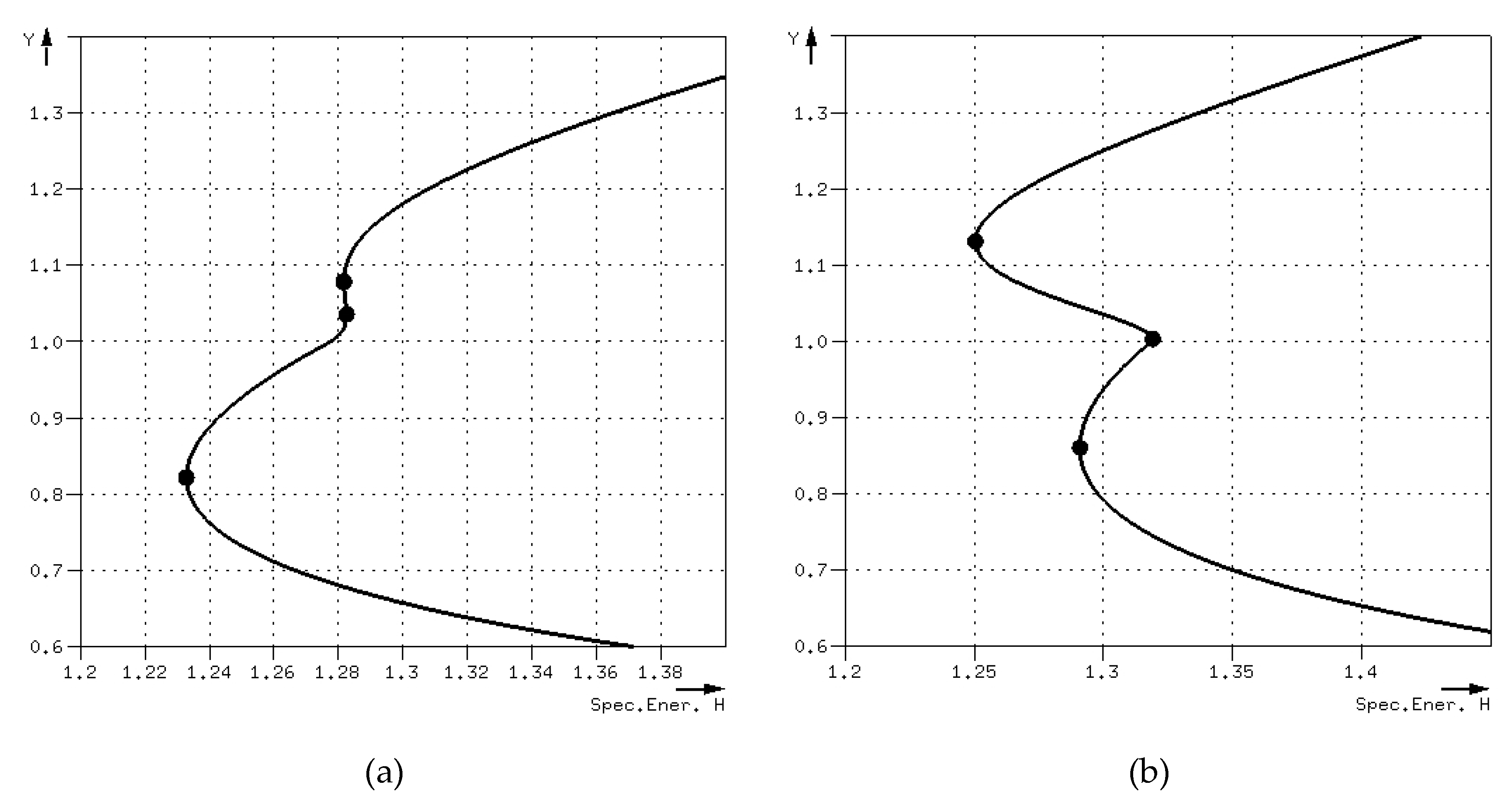
Dataset 2 consists of selected compound sections having each multiple critical depths. For each section, three critical depths were determined using the ACPA. When using HEC-RAS, although multiple critical depths were found, the one with the lowest energy was used. In all cases, this critical depth was the first (shallowest) determined using the ACPA. The values calculated with the two algorithms for this first critical depth are very similar, with a maximum difference of 0.0016 m and an average difference of 0.0005 m. Figure 12a shows the curve of the specific energy for one of these sections. The three critical depths calculated with the ACPA were 0.8219, 1.0358 and 1.0777m, appearing as black dots. The lowest depth coincides with the one found with HEC-RAS with a value of 0.8219m.
For the two-stage compound section presented in Figure 10, considering a discharge value of 2.5m3/s, the critical depths calculated were 0.86 m, 1.01 m and 1.129 m. These values agree with the respective ones calculated by Blalock and Sturm [2] for the same section and appear in Figure 12b together with the curve of the specific energy.
Dataset 3 consists of 62 natural sections having irregular shapes and being defined by multiple points. Most of the time, the curve of the specific energy is not continuous, due to reasons already explained. The critical depths calculated through ACPA were 1, 3, 5 or 7 for each section. From these critical depths, the one that had the minimum energy (CDMSE) was selected to be compared with the critical depth provided by HEC-RAS, as the CDMSE is the critical depth selected by the HEC-RAS’s algorithm, when more than one critical depths are located. The results of this comparison between the two algorithms can be classified in five different cases, depending on the number of the critical depths deriving from the ACPA and the difference (stated as “error”) between the CDMSE and the critical depth resulted from HEC-RAS. The tolerance selected for the classification was set at 0.1ft (0.03m). Differences lower than this tolerance are considered too small, that is to say that the critical depths compared are practically equal. More analytically, these five classifications were:
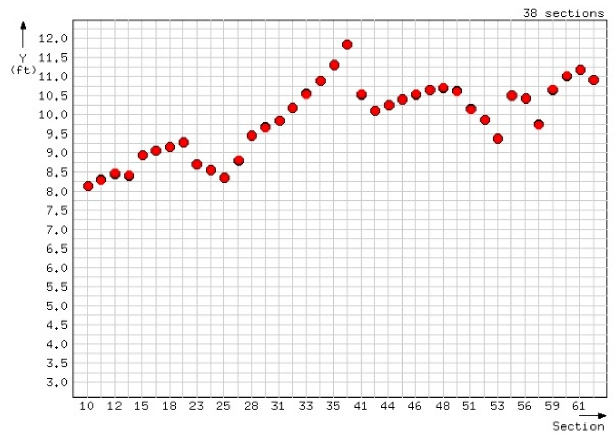
Case 1: There was only one critical depth. Its value agreed with the one resulted from HEC-RAS. Thirty-eight sections (i.e. 10–13, 15, 17–19, 23–26, 28, 30–35, 38, 41, 43–49, 51–54, 56, 57 and 59–62) fell into this case. Figure 13 presents their critical depths. The maximum error was 0.0167ft, while the average error was 0.0091ft. The black dots represent the values calculated through ACPA, while the red ones represent the values calculated through HEC-RAS.
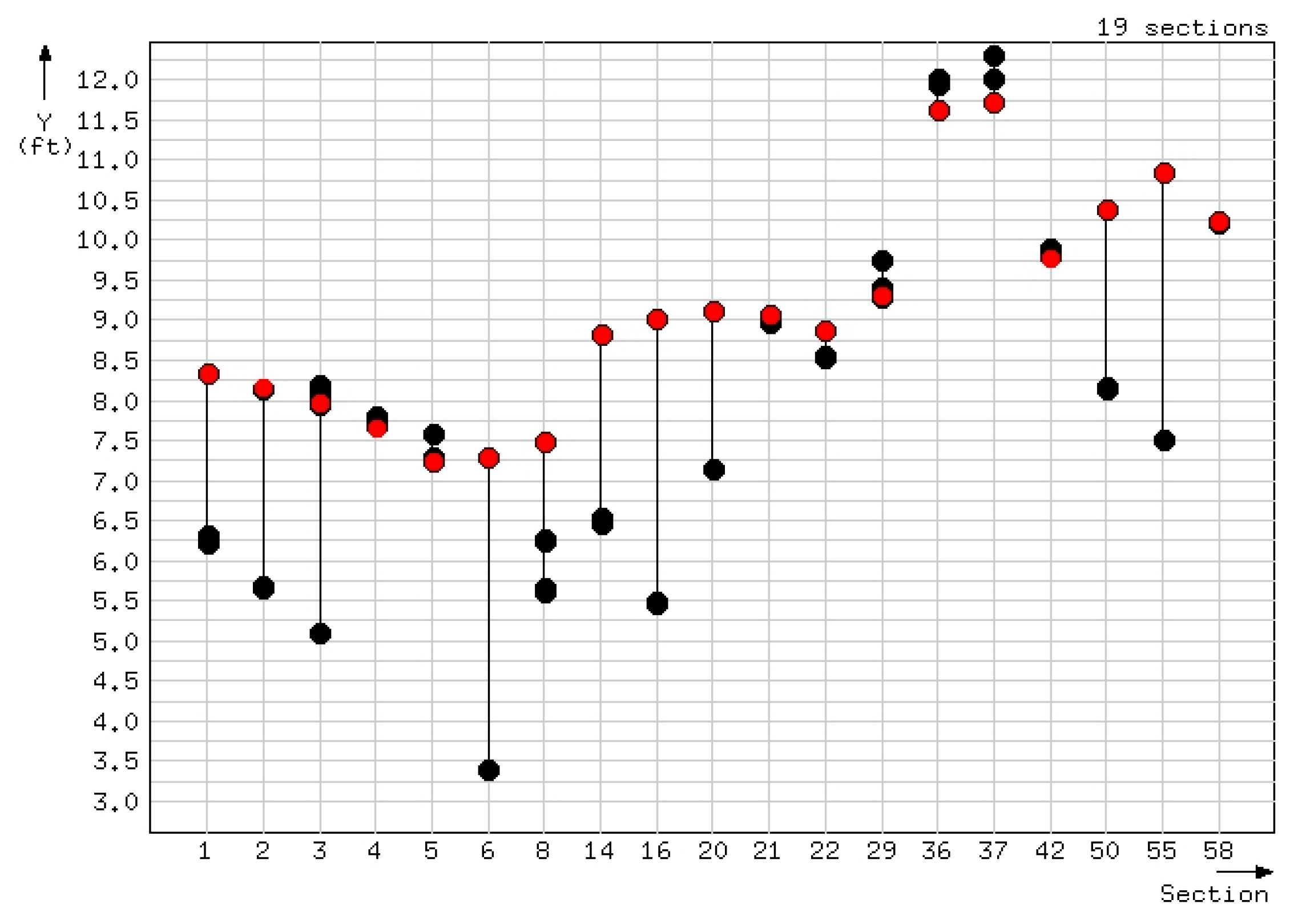
Case 2: There were multiple critical depths. The CDMSE agreed with the one resulted from HEC-RAS. Nineteen sections (i.e. 1–6, 8, 14, 16, 20–22, 29, 36, 37, 42, 50, 55 and 58) fell into this case. Figure 14 presents their critical depths. The maximum error was 0.0842ft, while average error was 0.0115ft. A dark vertical line is drawn from the lowest to the highest depth of each section.
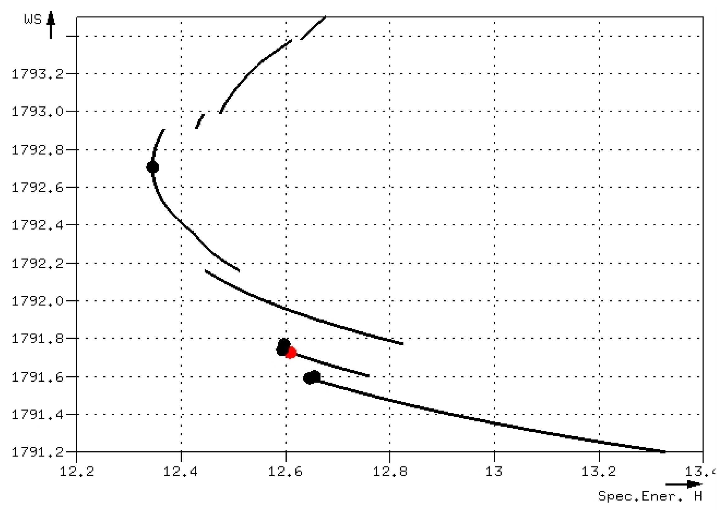
Case 3: There were multiple critical depths. One of them agreed with the one resulted from HEC-RAS, but it was not the CDMSE. Only section 40 fell into this case. Figure 15 presents its critical depths, together with the curve of the specific energy. The critical depth defined by HEC-RAS was 1,791.726ft but did not have the minimum energy, while the CDMSE was 1792.706ft. The error was 0.98ft.
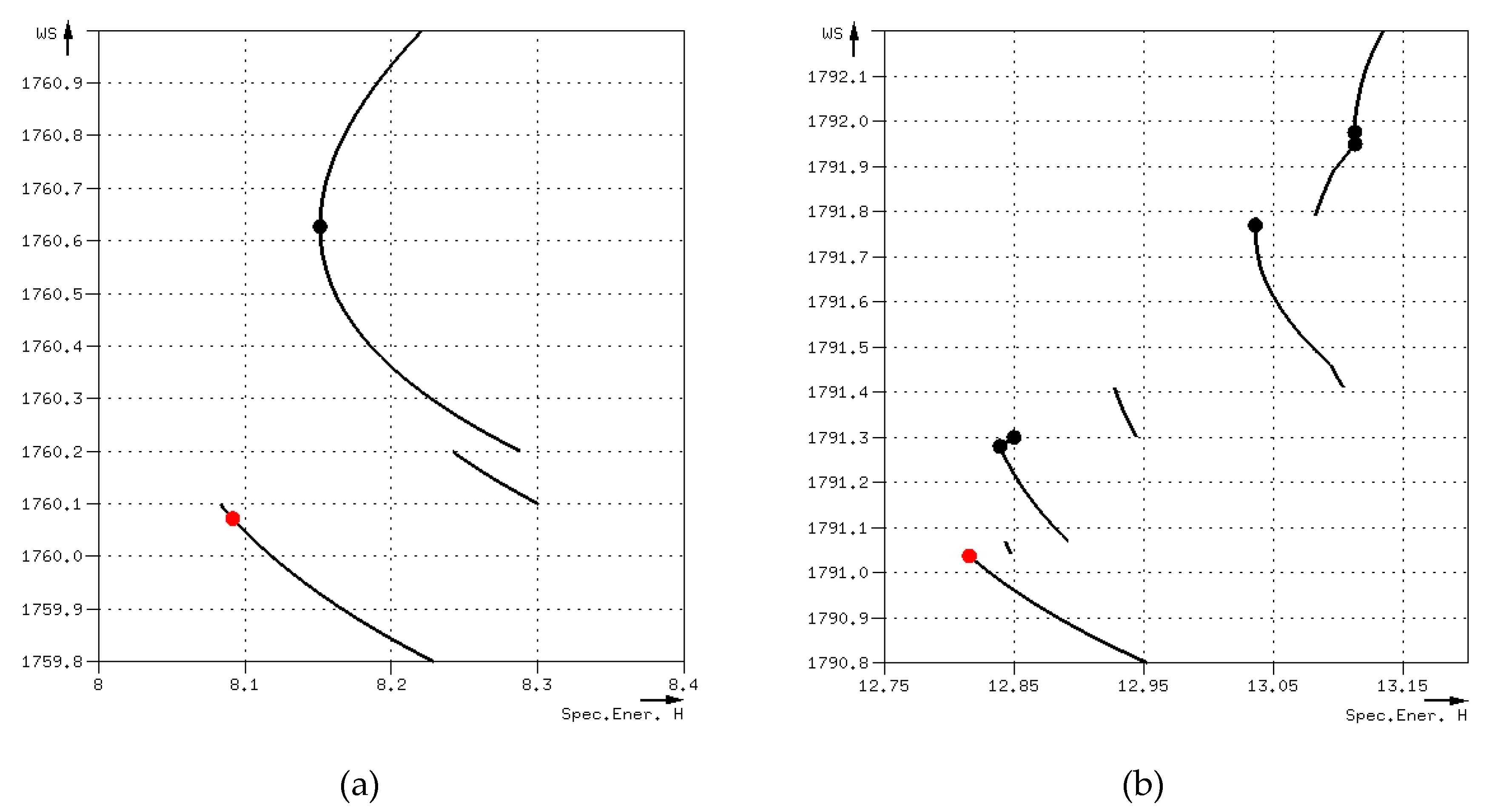
Case 4: There were multiple critical depths. None of them agreed with the one defined by HEC-RAS. Only two sections (i.e. 7, 39), fell into this case. Figure 16 presents their critical depths, together with the curves of the specific energy. The curve for section 39 was not continuous for several depths. In both sections the depth selected by HEC-RAS was not critical, since the slope of the specific energy curve before and after it was negative, and therefore the flow regime was supercritical. The error between CDMSE and HEC-RAS was 0.555ft for section 7 and 0.243ft for section 39.
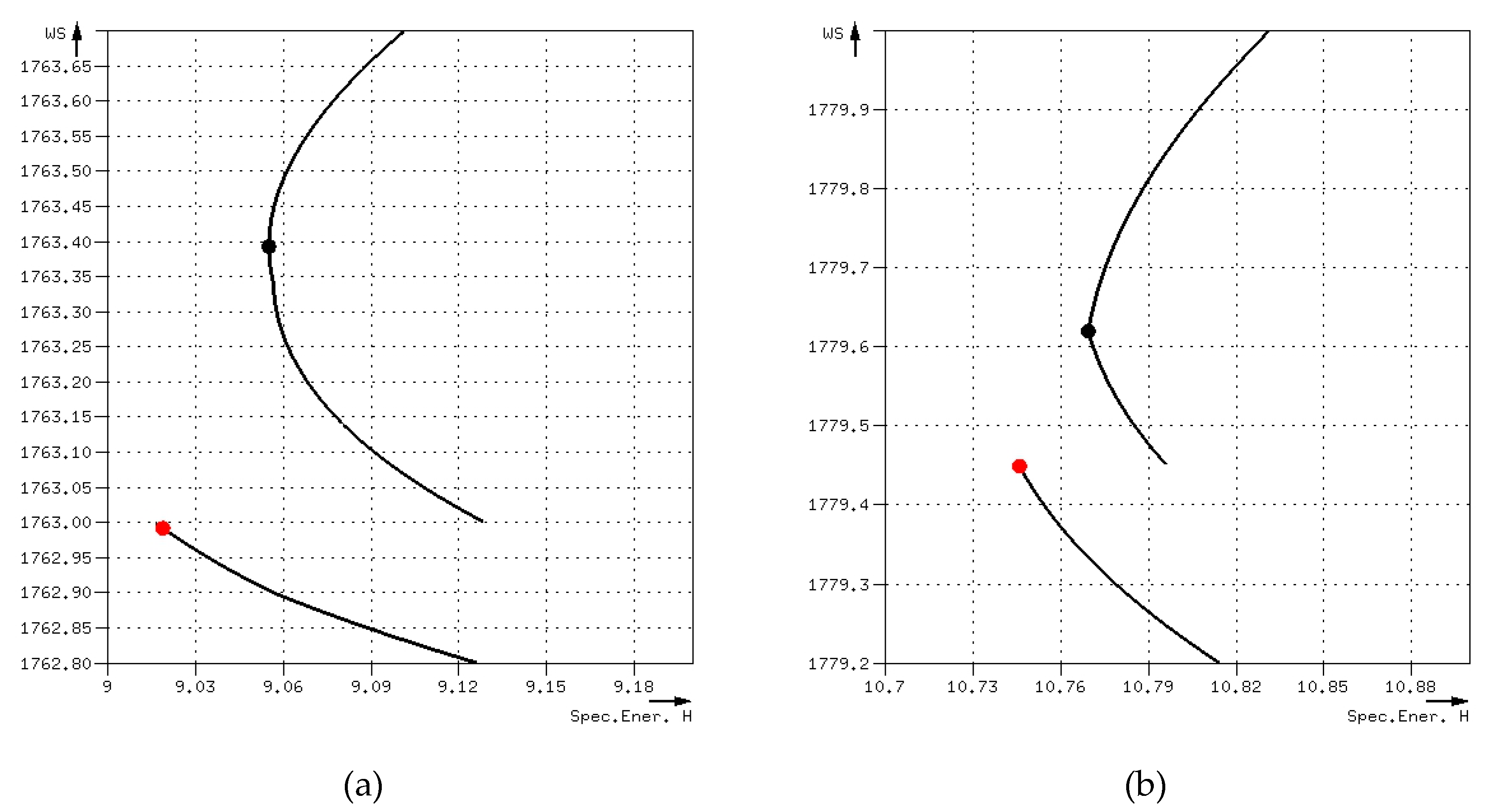
Case 5: There was only one critical depth. Its value did not agree with the one resulted from HEC-RAS. Two sections (i.e. 9, 27) fell into this case. Figure 17 presents their critical depths, together with the curves of the specific energy. In both cases the depth selected was not critical since the slope of the specific energy curve before and after it, was negative, thus the flow regime was supercritical. The error between CDMSE and HEC-RAS was 0.4 ft for section 9 and 0.171ft for section 27.
The comparison analysis of the critical depths defined by both ACPA and HEC-RAS for dataset 4 had the same outputs as the one performed for dataset 3. The same five cases/groups were formed:
Case 1: There was only one critical depth. Its value agreed with the one resulted from HEC-RAS. Forty-one sections (i.e. 4, 17–19, 21–38, 42–49, 51–54 and 56–62) fell into this case. The maximum error was 0.0307ft, while the average error was 0.0071ft.
Case 2: There were multiple critical depths. The CDMSE agreed with the one resulted from HEC-RAS. Thirteen sections (i.e. 2, 3, 7, 8, 10, 11, 13, 16, 20, 39, 40, 50 and 55) fell into this case. The maximum error was 0. 065ft, while the average error was 0.0121ft.
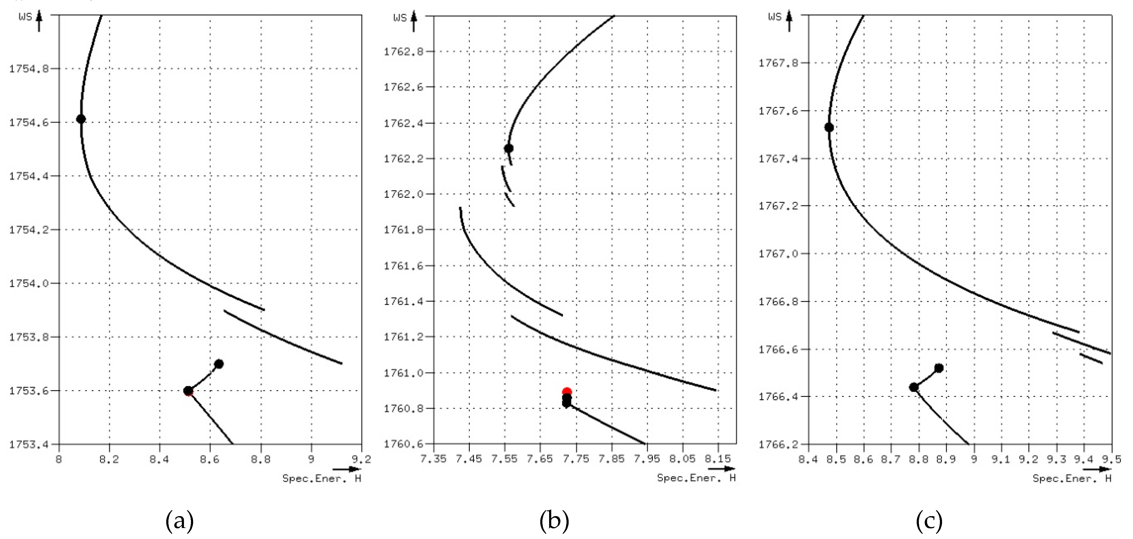
Case 3: There were multiple critical depths. One of them agreed with the one resulted from HEC-RAS, but it was not the CDMSE. Six sections (i.e. 1, 5, 6, 9, 14 and 41) fell into this case. Figure 18a–c present the critical depths for the sections 1, 9 and 14 respectively, together with the curves of specific energy. The error between CDMSE and HEC-RAS was 1.016ft (sect.1), 0.367ft (sect.5), 0.175ft (sect.6), 1.366ft (sect.9), 1.09ft (sect.14) and 0.101ft (sect.41). They were all quite big, especially for section 9.
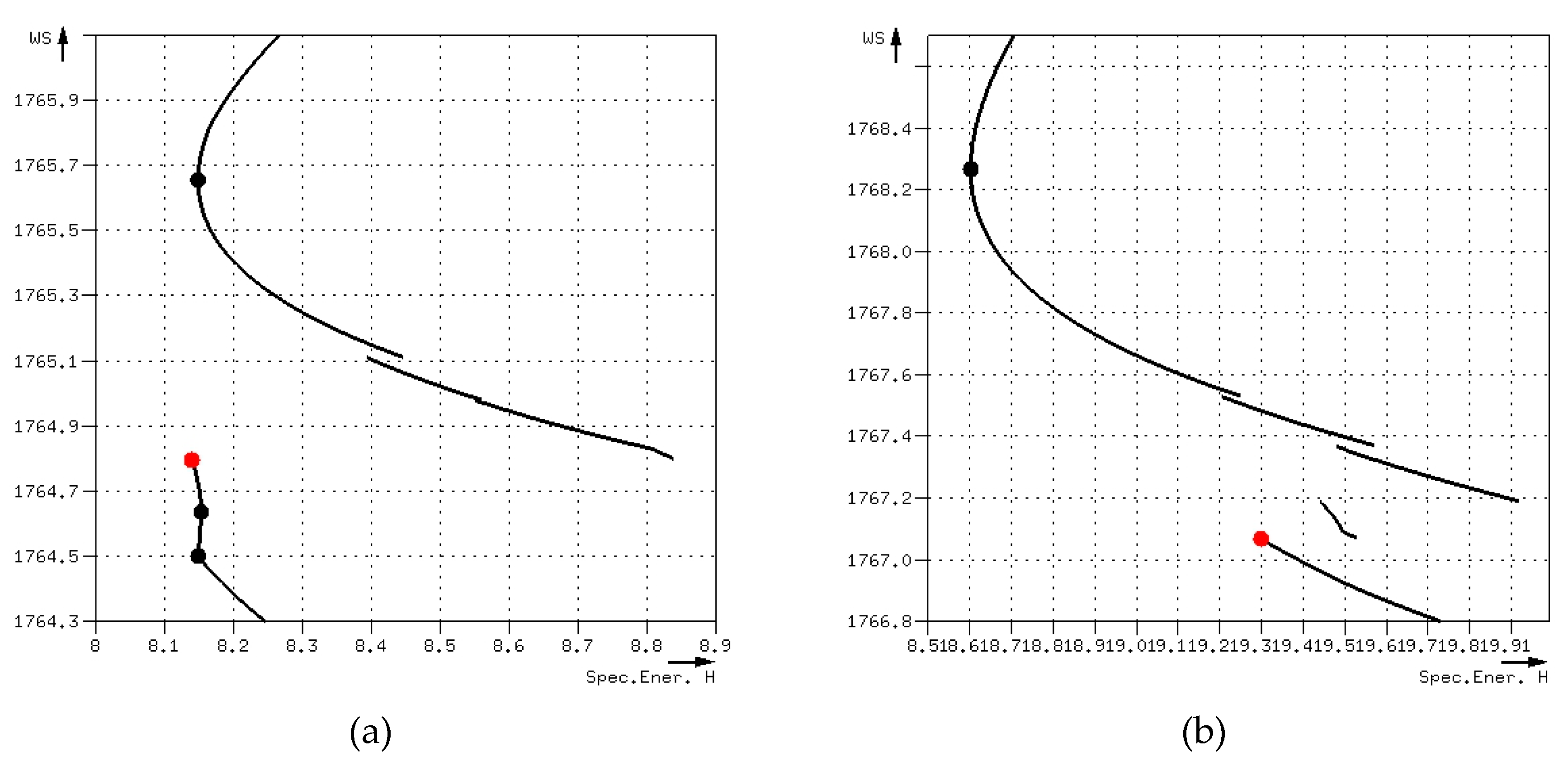
Case 4: There were multiple critical depths. None of them agreed with the one defined by HEC-RAS. Only section 12 fell into this case. Figure 19a presents its critical depths. The error between CDMSE and HEC-RAS was 0.86ft.
Case 5: There was only one critical depth. Its value did not agree with the one resulted from HEC-RAS. Only section 15 fell into this case. Figure 19b presents its critical depths. The error between CDMSE and HEC-RAS was 1.198ft.
5. Discussion
The slope of the curve of the specific energy for any section at any depth of flow determines the flow regime at this depth. Critical is the depth where the flow changes regime from supercritical to subcritical or vice versa. Consequently, the slope of the curve before the critical depth must have the opposite sign to the slope after it. Based on this criterion, the whole curve can be checked and the locations fulfilling this condition will be critical depths. In compound and natural sections with overbanks and multiple friction zones, the shape of this curve is complex and is often not continuous, therefore cannot be approximated. In this study, the points of discontinuity were determined and an algorithm was developed in order for all segments of the curve to be approximated by cubic polynomials. This allowed the analytic calculation of the specific energy value at any depth. Furthermore, it allowed the determination of the critical depth locations.
This adaptive cubic polynomials algorithm (ACPA) developed was validated through four different datasets. Thorough examination of the critical depths calculated and of the curve of the specific energy in each section proved that these depths are indeed critical ones, fulfilling the abovementioned condition regarding the sign of the slope of the specific energy curve.
The algorithm used by HEC-RAS for the determination of the critical depths is based on the minimum specific energy criterion. Many researchers have confirmed that this definition is not sufficient enough when compound channels are being studied [22,23,24]. Due to the discontinuities present in many natural sections, one location might be a local minimum without being a valid critical depth at the same time (Figure 17a). Apart from that, the whole range of elevations is being evenly divided in thirty segments and each one is being checked in order the general location of a critical depth to be located. In complex sections actually, this process may be too sparse, and the critical depth may be skipped or even omitted.
The comparison analysis of the two algorithms showed that at prismatic sections, such as in dataset 1, the results are identical. For the two stage compound sections, such as in dataset 2, with multiple critical depths, ACPA locates them all, while HEC-RAS locates only the one with the minimum specific energy. For more complex sections, such as datasets 3 and 4, HEC-RAS occasionally fails to identify a valid critical depth or finds one that is not the one with the minimum specific energy, as it should. Five sections of dataset 3 and eight of dataset 4 have been assigned a false critical depth yielding 8% and 12.9% possibility for a wrong answer. If such a faulty critical depth is used as a boundary condition for GVF (gradually varied flow) calculations, then at least the results nearby will be distorted.
6. Conclusions
Although explicit solutions for the determination of the critical depth are possible for prismatic and parabolic channels [25], for natural channels this is impossible due to their inherent complexity. In this study, an algorithm which approximates the specific energy curve of natural or compound sections with multiple cubic polynomials is presented. The segments for each polynomial are automatically found and, if necessary, they are subdivided in order to achieve an error free approximation. Then, the roots of the derivatives of these polynomials are determined. These are the critical depths of the section. In addition, the slope of the polynomials is checked to locate any additional critical depths that lie at the end of the segments. This algorithm, unlike iterative algorithms that may or may not converge, has the benefit of providing solutions every time it is used. Moreover, it has been proven that in all cases where it was tested, it provided accurate results.
Apart from the critical depths, the Froude number at any elevation can easily be calculated by evaluating the derivative of the corresponding cubic polynomial which contains the given elevation.
The algorithm has been tested and compared with HEC-RAS regarding the critical depths defined. In most cases, the results do agree. In cases where non-negligible errors were found, it was proven that ACPA’s results were more accurate compared to those of HEC-RAS. This is due to the fact that HEC-RAS uses an algorithm which is more suitable for simple sections. On the contrary, in compound and natural sections, the multiple critical depths existing cannot be located through HEC-RAS as the algorithm HEC-RAS used determines only one critical depth.
Author Contributions
E.K. provided the guidelines and the tools of the study; I.P. and E.K. conceived and designed the scenarios studied; I.P. analyzed the data; I.P. and E.K. wrote the paper. V.K. reviewed and finalized the paper. All authors have read and agreed to the published version of the manuscript.
Funding
This research received no external funding.
Conflicts of Interest
The authors declare no conflict of interest.
References
- Henderson, F.M. Open Channel Flow; The Macmillan Co.: New York, NY, USA, 1969. [Google Scholar]
- Blalock, M.E.; Sturm, T.W. Minimum Specific Energy in Compound Channel. J. Hydraul. Div. 1981, 107, 699–717. [Google Scholar]
- Blalock, M.E.; Sturm, T.W. Closure of Minimum Specific Energy in Compound Channel. J. Hydraul. Div. 1983, 109, 483–486. [Google Scholar] [CrossRef]
- Bakhmeteff, B.A. Hydraulics of Open Channels; McGraw-Hill Book Co., Inc.: New York, NY, USA, 1932. [Google Scholar]
- Schoellhamer, D.H.; Peters, J.C.; Larok, B.E. Subdivision Froude Number. Hydraul. Eng. 1985, 111, 1099–1104. [Google Scholar] [CrossRef]
- Chow, V.T. Open-Channel Hydraulics; McGraw-Hill Book Company: New York, NY, USA, 1959. [Google Scholar]
- Konemann, N. Discussion of Blalock and Sturm [1981]. J. Hydraul. Div. 1982, 108, 462–464. [Google Scholar]
- Petryk, S.; Grant, E.U. Critical Flow in Rivers with Flood Plains. J. Hydraul. Div. 1978, 104, 583–594. [Google Scholar]
- Chaudhry, M.H.; Bhallamudi, S.M. Computation of Critical Depth in Symmetrical Compound Channels. Hydraul. Res. 1988, 26, 377–396. [Google Scholar] [CrossRef]
- Samuels, P.G. Cross section location in one-dimensional models. In Proceedings of the International Conference on River Flood Hydraulics, At Wallingford, UK, 17–20 September 1990; White, W.R., Ed.; John Wiley: Chichester, UK; pp. 339–350. [Google Scholar]
- Pramanik, N.; Panda, R.K.; Sen, D. One dimensional hydrodynamic modeling of river flow using Dem extracted river cross sections. Water Resour. Manag. 2010, 24, 835–852. [Google Scholar] [CrossRef]
- Pilotti, M. Extraction of cross sections from digital elevation model for one-dimensional dam-break wave propagation in mountain valleys. Water Resour. Res. 2016, 52, 52–68. [Google Scholar] [CrossRef] [Green Version]
- O’Callaghan, J.F.; Mark, D.M. The extraction of drainage networks from digital elevation data. Comput. Vis. Graph. Image Process. 1984, 28, 323–344. [Google Scholar] [CrossRef]
- Jenson, S.K.; Domingue, J.O. Extracting topographic structure from digital elevation data for geographic information system analysis. Photogramm. Eng. Remote Sens. 1988, 54, 1593–1600. [Google Scholar]
- Tarboton, D.G.; Bras, R.L.; Rodriguez-Iturbe, I. On the extraction of channel networks from digital elevation data. Hydrol. Process. 1991, 5, 81–100. [Google Scholar] [CrossRef]
- Garbrecht, J.; Martz, L. Grid size dependency of parameters extracted from digital elevation models. Comput. Geosci. 1994, 20, 85–87. [Google Scholar] [CrossRef]
- Hydrologic Engineering Center. HEC-RAS River Analysis System, Computer Program; Version 5.0.7.; US Army Corps of Engineers, Institute of Water Resources: Davis, CA, USA, 2019.
- Hydrologic Engineering Center. HEC-RAS River Analysis System, Hydraulic Reference Manual; Version 5.0; US Army Corps of Engineers, Institute of Water Resources: Davis, CA, USA, 2016.
- Hydrologic Engineering Center. HEC-RAS River Analysis System, Applications Guide; Version 5.0; US Army Corps of Engineers, Institute of Water Resources: Davis, CA, USA, 2016.
- Hydrologic Engineering Center. HEC-2 Water Surface Profile User’s Manual; US Army Corps of Engineers, Institute of Water Resources: Davis, CA, USA, 1991.
- Hydrologic Engineering Center. HEC-2 Water Surface Profiles Computer Program; US Army Corps of Engineers, Institute of Water Resources: Davis, CA, USA, 1991.
- Chaudhry, M.H. Open-Channel Flow; Springer: New York, NY, USA, 2008. [Google Scholar]
- Subramanya, K. Flow in Open Channels; Tata McGraw-Hill: New Delhi, India, 2009. [Google Scholar]
- Vatankhah, A.R. Multiple-Critical Depth Occurrence in Two-Stage Cross-Sections: Effect of Side Slope Change. Hydrol. Eng. 2013, 18, 722–728. [Google Scholar] [CrossRef] [Green Version]
- Vatankhah, A.R. Explicit solutions for critical and normal depths in trapezoidal and parabolic open channels. Ain Shams Eng. J. 2013, 4, 17–23. [Google Scholar] [CrossRef] [Green Version]
Figure 1.
Natural section with three regions, main channel, left and right overbanks.

Figure 2.
(a) Natural section with flat region; (b) the wetted perimeter P is discontinuous.

Figure 3.
(a) Two parallel flows with separate conveyances K1 and K2. Total conveyance K = K1 + K2; (b) flows joined up to a single flow with a single conveyance K.
Figure 3.
(a) Two parallel flows with separate conveyances K1 and K2. Total conveyance K = K1 + K2; (b) flows joined up to a single flow with a single conveyance K.

Figure 4.
(a) Successive elevations of a natural section; (b) The trapezoidal subsections between two successive elevations; (c) The wetted perimeters of the subsections.
Figure 4.
(a) Successive elevations of a natural section; (b) The trapezoidal subsections between two successive elevations; (c) The wetted perimeters of the subsections.

Figure 5.
(a) Curve is flat on edge A and highly curved on edge B. (b) Curve has been subdivided in five sub-curves which fulfill certain criteria of “flatness”.
Figure 5.
(a) Curve is flat on edge A and highly curved on edge B. (b) Curve has been subdivided in five sub-curves which fulfill certain criteria of “flatness”.

Figure 6.
Part of the specific energy curve. The segments between successive elevations are continuous and differentiable.
Figure 6.
Part of the specific energy curve. The segments between successive elevations are continuous and differentiable.

Figure 7.
Specific energy (H) calculated at various elevations (y).

Figure 8.
Critical points at the ends of segments. (a) Local minimum, specific energy with continuity. (b) Local maximum, specific energy without continuity.
Figure 8.
Critical points at the ends of segments. (a) Local minimum, specific energy with continuity. (b) Local maximum, specific energy without continuity.

Figure 9.
Non-symmetric two stage trapezoidal compound section.

Figure 10.
Two stage rectangular compound section.

Figure 11.
Sections of dataset 3 (a) section 1 with 61 points; (b) section 7 with 61 points; (c) section 13 with 69 points; and (d) section 19, with 85 points.
Figure 11.
Sections of dataset 3 (a) section 1 with 61 points; (b) section 7 with 61 points; (c) section 13 with 69 points; and (d) section 19, with 85 points.

Figure 12.
Specific energy and critical depths of: (a) a typical compound section of dataset 2; (b) the compound section of Figure 10.
Figure 12.
Specific energy and critical depths of: (a) a typical compound section of dataset 2; (b) the compound section of Figure 10.

Figure 13.
Dataset 3: Critical depths of case 1 sections.

Figure 14.
Dataset 3: Critical depths of case 2 sections.

Figure 15.
Dataset 3: Critical depths of case 3 section.

Figure 16.
Dataset 3: Critical depths of case 4 (a) section 7 and (b) section 39.

Figure 17.
Dataset 3: Critical depths of case 5 (a) section 9 and (b) section 27.

Figure 18.
Dataset 4: Critical depths of case 3 (a) section 1, (b) section 9 and (c) section 14.

Figure 19.
Dataset 4: Critical depths for (a) case 4 section 12 and (b) case 5 section 15.


Table 1.
Outline of Adaptive Cubic Polynomial Algorithm (ACPA).
|
Table 2.
Comparison analysis results for 2251 elevations (Differences in computed hydraulic parameters).
Table 2.
Comparison analysis results for 2251 elevations (Differences in computed hydraulic parameters).
| Parameter | Symbol | Max. Dif. | Max. Dif. (%) | Avg. Dif. | Avg. Dif. (%) |
|---|---|---|---|---|---|
| Total cross-sectional area | A | 0.08 | 0.0005 | 0.02 | 0.001 |
| Kinetic energy correction factor | a | 0.034 | 0.626 | 0.00 | 0.002 |
| Specific energy | H | 38.67 | 0.057 | 0.18 | 0.004 |
Table 3.
Differences between critical depths computed with ACPA and HEC-RAS for dataset 3.
| Section Index | Case | Difference |
|---|---|---|
| 7 | 4 | 0.555 |
| 9 | 5 | 0.4 |
| 27 | 5 | 0.171 |
| 39 | 4 | 0.243 |
| 40 | 3 | 0.98 |
Table 4.
Differences between critical depths computed with ACPA and HEC-RAS for dataset 4.
| Section Index | Case | Difference |
|---|---|---|
| 1 | 3 | 1.016 |
| 5 | 3 | 0.367 |
| 6 | 3 | 0.175 |
| 9 | 3 | 1.366 |
| 12 | 4 | 0.86 |
| 14 | 3 | 1.09 |
| 15 | 5 | 1.198 |
| 41 | 3 | 0.101 |
© 2020 by the authors. Licensee MDPI, Basel, Switzerland. This article is an open access article distributed under the terms and conditions of the Creative Commons Attribution (CC BY) license (http://creativecommons.org/licenses/by/4.0/).
Share and Cite
MDPI and ACS Style
Petikas, I.; Keramaris, E.; Kanakoudis, V. Calculation of Multiple Critical Depths in Open Channels Using an Adaptive Cubic Polynomials Algorithm. Water 2020, 12, 799. https://doi.org/10.3390/w12030799
AMA Style
Petikas I, Keramaris E, Kanakoudis V. Calculation of Multiple Critical Depths in Open Channels Using an Adaptive Cubic Polynomials Algorithm. Water. 2020; 12(3):799. https://doi.org/10.3390/w12030799
Chicago/Turabian StylePetikas, Ioannis, Evangelos Keramaris, and Vasilis Kanakoudis. 2020. "Calculation of Multiple Critical Depths in Open Channels Using an Adaptive Cubic Polynomials Algorithm" Water 12, no. 3: 799. https://doi.org/10.3390/w12030799
Note that from the first issue of 2016, this journal uses article numbers instead of page numbers. See further details here.