Real-Time Probabilistic Flood Forecasting Using Multiple Machine Learning Methods

Abstract

Probabilistic flood forecasting, which provides uncertain information in the forecasting of floods, is practical and informative for implementing flood-mitigation countermeasures. This study adopted various machine learning methods, including support vector regression (SVR), a fuzzy inference model (FIM), and the k-nearest neighbors (k-NN) method, to establish a probabilistic forecasting model. The probabilistic forecasting method is a combination of a deterministic forecast produced using SVR and a probability distribution of forecast errors determined by the FIM and k-NN method. This study proposed an FIM with a modified defuzzification scheme to transform the FIM’s output into a probability distribution, and k-NN was employed to refine the probability distribution. The probabilistic forecasting model was applied to forecast flash floods with lead times of 1–3 hours in Yilan River, Taiwan. Validation results revealed the deterministic forecasting to be accurate, and the probabilistic forecasting was promising in view of a forecasted hydrograph and quantitative assessment concerning the confidence level.

1. Introduction

A real-time flood forecasting model is an essential nonstructural component in a flood warning system. It can provide timely forecasting information to authorities and the public with sufficient time for preparation and useful information for implementing flood-mitigation countermeasures. Flood forecasting is often performed deterministically [1], which means that a single estimate of flood discharge or stage is predicted. However, a deterministic forecast can leave users with an illusion of certainty, which can lead them to take inadequate measures [2]. Therefore, a probabilistic forecast that specifies a probability distribution pertaining to the predictand is more practical and has thus gained attention in flood forecasting [1].

Many methods are used to perform probabilistic flood forecasting. For example, the Bayesian forecasting system that integrates prior and posterior information using Bayes’ theorem has been adopted [3,4,5,6]. Furthermore, multimodel ensemble methods have been used, which produce several forecasts based on different models [7,8,9]. Moreover, researchers have adopted generalized likelihood uncertainty estimation, which is based on the idea that many different parameters may yield equally satisfactory estimates [10,11,12,13,14,15]. The present study adopted a method that combines deterministic forecasts and the probability distribution of forecast errors to produce probabilistic forecasts [1]. Such a method was adopted because forecast-error data can quantify the total uncertainty of forecasting. Montanari and Brath [16], Tamea et al. [17], and Weerts et al. [18] have used similar methods based on processing past forecast-error data to produce probability distributions for future forecasts. On the basis of the combined method in this study, various machine learning methods were applied to achieve probabilistic forecasting.

Numerous machine learning methods have been widely applied in hydrologic forecasting. A classic approach is to apply artificial neural networks to tasks such as radar rainfall estimation [19,20], flood forecasting [21,22], and reservoir inflow prediction [23,24]. A machine learning method that has recently become popular is the support vector machine (SVM) approach, which is capable of regression and classification. The SVM has been used for flood forecasting [25,26,27], daily rainfall downscaling [28,29], mining informative hydrologic data [30,31], and typhoon rainfall forecasting [32,33]. Moreover, various fuzzy models based on fuzzy set theory have been adopted in hydrologic forecasting; for example, rainfall forecasting [34,35], river level forecasting [36,37], and flood discharge forecasting [38,39,40]. The nonparametric k-nearest neighbors (k-NN) method is a simple and useful algorithm for data selection, classification, and regression. The k-NN method has been widely applied in hydrology, such as in short-term rainfall prediction [41], reservoir inflow forecasting [42], climate change scenario simulation [43], and hydrologic data generation [44].

This study applied multiple machine learning methods to achieve probabilistic flood-stage forecasting. The SVM was used to develop a deterministic forecasting model to forecast deterministic flood stages. Furthermore, this study proposed a fuzzy inference model (FIM) with a modified defuzzification scheme to deduce the probability distribution of forecast errors. In addition, the k-NN method was applied to smooth the derived probability distribution. Combining deterministic flood-stage forecasting and the probability distribution of forecast errors yielded probabilistic flood-stage forecasts. The probabilistic forecasting model was applied to forecast flood stages in Taiwan’s Yilan River. Validation results regarding actual flash flood events proved the capability of the proposed model in view of the forecasted hydrograph and a quantitative assessment concerning the confidence level.

This remainder of this paper is organized as follows. Section 2 provides a brief introduction to the probabilistic forecasting method and machine learning methods employed in this study. Section 3 describes the development and forecasting of the SVR deterministic forecasting model as well as the study area and flood events. Section 4 presents the use of the FIM and k-NN method to derive the probability distribution of forecast errors and the results of probabilistic forecasting. Finally, Section 5 presents the study’s conclusions.

2. Probabilistic Forecasting and Machine Learning Methods

2.1. Probabilistic Forecasting Method

This study applied the probabilistic forecasting method based on the methodology proposed by Chen and Yu [1], but modified it using the k-NN method to refine the probability distribution. A probabilistic forecast was obtained by combining deterministic forecasting with the probability distribution of forecast errors. A concise description of the method is presented as follows, and the detailed methodology can be found in Chen and Yu [1].

The forecast error ($E$) is defined as the difference between the deterministic forecast ($F$) and the observation ($O$).

$$E=F-O$$

(1)

Given that $O$ represents an observation without uncertainty, the variance of deterministic forecast $F$ is the same as that of the error forecast.

$$\mathrm{var}\left(F\right)=\mathrm{var}\left(E\right)$$

(2)

Thus, the uncertainty of the forecast can be deduced from the uncertainty of forecast errors. Then, the probability distribution of the forecast ${\mathsf{\Pi }}_F$ can be derived by adding the probability distribution of forecast errors ${\mathsf{\Pi }}_E$ into the single deterministic forecast $F$.

$${\mathsf{\Pi }}_F=F+{\mathsf{\Pi }}_E$$

(3)

Consequently, the probabilistic forecasting results can be demonstrated as a confidence interval with a certain confidence level from the probability distribution ${\mathsf{\Pi }}_F$.

2.2. Support Vector Regression

This study used SVR to provide deterministic forecasts. SVR is a regression procedure based on a SVM that utilizes the structural risk minimization induction principle to minimize the expected risk based on limited data [45]. Detailed descriptions of SVM theory can be found in the literature [26,46]. A brief methodology of SVR is described as follows.

SVR finds the optimal nonlinear regression function $f\left(x\right)$ according to r data sets $\left(x_i,y_i\right)$, where $x_i$ are input vectors and $y_i$ are corresponding output variables (i = 1, …, r). The SVR function can be written as

$$f\left(x\right)=w·\mathsf{\Phi }\left(x\right)+b$$

(4)

where $w$ is the weight vector, $b$ is bias, and $\mathsf{\Phi }$ is a nonlinear function that maps the original data onto a higher dimensional space, in which the input–output data can exhibit linearity. The calibration of the regression function involves an error tolerance ε when calculating the loss $L$, which is defined using Vapnik’s ε-insensitive loss function.

$$L\left(y_i\right)=\{\begin{array}{cc}0,& \mathrm{for}\left|y_i-\left(\mathrm{w}\times \mathsf{\Phi }\left({\mathrm{x}}_i\right)+b\right)\right|<\epsilon \\ \left|y_i-\left(\mathrm{w}\times \mathsf{\Phi }\left({\mathrm{x}}_i\right)+b\right)\right|-\epsilon ,& \mathrm{for}\left|y_i-\left(\mathrm{w}\times \mathsf{\Phi }\left({\mathrm{x}}_i\right)+b\right)\right|\ge \epsilon \end{array}$$

(5)

This regression problem can be formulated as a convex optimization problem, in which a dual set of Lagrange multipliers, ${\alpha }_i$ and ${\alpha }_i^{*}$, are introduced to solve the problem by applying a standard quadratic programming algorithm. As a result, the SVR function can be written as

$$f\left(x\right)={{\displaystyle \sum }}_{i,j=1}^r\left({\alpha }_i-{\alpha }_i^{*}\right)\mathsf{\Phi }{\left(x_i\right)}^T·\mathsf{\Phi }\left(x_j\right)+b$$

(6)

Then, a kernel function $K\left(x_i,x_j\right)=\mathsf{\Phi }{\left(x_i\right)}^T·\mathsf{\Phi }\left(x_j\right)$ is used to yield the inner products in the higher dimensional space to ease the calculation. This study used the radial basis function kernel with a parameter $\gamma$ as the kernel function.

$$K\left(x_i,x_j\right)=\exp \left(-\gamma {\left|x_i-x_j\right|}^2\right)$$

(7)

From Equation (6), only data with nonzero Lagrange multipliers $\left({\alpha }_i-{\alpha }_i^{*}\right)$ are used in the final regression function, and these data are termed support vectors. Finally, the regression function can be formulated as

$$f\left(x\right)={{\displaystyle \sum }}_{k=1}^m\left({\alpha }_k-{\alpha }_k^{*}\right)K\left(x_k,x\right)+b$$

(8)

where $x_k$ denotes the support vector and $m$ represents the number of support vectors.

2.3. Fuzzy Inference Model

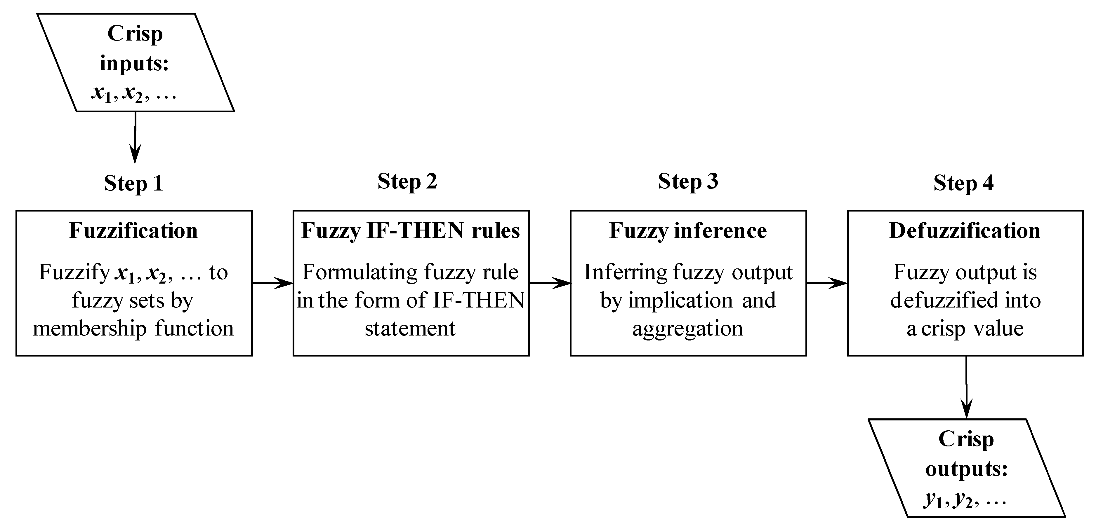
This study adopted an FIM with a defuzzification method to infer the probability distribution of forecast errors (the difference between the observation and forecast). The FIM included four steps (Figure 1), which are described as follows.

(1) Fuzzification

Fuzzification is a process that converts a crisp value (numerical value) to a fuzzy variable through a fuzzy membership function. Some membership functions are widely used, such as the triangular, trapezoidal, and Gaussian functions. In this study, the Gaussian membership function (Equation (9)) was used because of its easier differentiability compared with the triangular membership function [1]. The Gaussian function also exhibits superior performance compared with the trapezoidal function, and also demonstrates a smoother transition in its intervals [47].

$$\mu \left(x\right)=\exp \left(\frac{-{\left(x-m\right)}^2}{2{\sigma }^2}\right)$$

(9)

where $\mu$ is the membership grade of the crisp input $x$; $\sigma$ is the dispersion of the function; and $m$ is the center of the function.

(2) Fuzzy IF-THEN rules

The IF-THEN rule is used to formulate the conditional statement in the FIM. The fuzzy IF-THEN rule can be expressed as follows:

$$\begin{gathered} \mathrm{IF} \left(x_1\mathrm{is}{A}_1\right)\mathrm{and}\left(x_2\mathrm{is}{A}_2\right)\mathrm{and}\cdots \mathrm{and}\left(x_p\mathrm{is}{A}_p\right) \\ \mathrm{THEN} \left(y_1\mathrm{is}{B}_1\right)\mathrm{and}\left(y_2\mathrm{is}{B}_2\right)\mathrm{and}\cdots \mathrm{and}\left(y_q\mathrm{is}{B}_q\right) \end{gathered}$$

(10)

where $x_i$ (i = 1, 2, …, p) and $y_j$ (j = 1, 2, …, q) indicate the crisp input and output variables, respectively; and $A_i$ (i = 1, 2, …, p) and $B_j$ (j = 1, 2, …, q) are fuzzy sets. The IF part of the rule is called the antecedent or premise, and the THEN part is the consequence or conclusion.

(3) Fuzzy inference

Fuzzy inference calculates the similarity between crisp inputs and fuzzy sets in fuzzy rules. It involves two procedures, namely implication and aggregation. Implication generates a fuzzy set in the consequence part for each fuzzy rule, whereas aggregation integrates the output fuzzy sets in all fuzzy rules into an aggregated fuzzy set. More details can be found in Yu and Chen [48] and Chen [49].

(4) Defuzzification

The fuzzy output obtained in the previous step is an aggregated fuzzy set that should be defuzzified to a crisp value $y^{*}$.

The centroid method, which directly computes the crisp output as a weighted average of membership grades, was used in the present study.

$$y^{*}=\frac{{{\displaystyle \sum }}_{i=1}^n{\mu }_i\times y_i}{{{\displaystyle \sum }}_{i=1}^n{\mu }_i}$$

(11)

where ${\mu }_i$ is the fuzzy membership grade of the output variable $y_i$ of the i-th rule and n is the number of rules.

2.4. Defuzzification Into a Probability Distribution

The higher value of ${\mu }_i$ in Equation (11) indicates that the $y_i$ of the i-th rule imposes a higher weight of influence on the output $y^{*}$. Chen and Yu [1] proposed a probability interpretation of defuzzification on the basis of basic defuzzification distribution transformation [50]. Thus, the defuzzification process in the FIM can be converted to produce a probability distribution. For the detailed theory and process of defuzzification into a probability distribution, please refer to Chen and Yu [1].

2.5. k-Nearest Neighbors Method

The k-NN method, an effective nonparametric technique, was utilized in this study to smooth the derived probability distribution from the previous step because it may have a rough shape. The k-NN algorithm typically picks a certain number of data items that are closer to the object. Given an object data vector of $\mathit{z}=\left(z_1,z_2,\cdots ,z_m\right)$, the k-NN algorithm selects k data items that are nearest to the object according to the similarity or distance $D$ from the candidate data$z\prime$ to the object data $z$.

$$D=\Vert \mathit{z}-\mathit{z}\prime \Vert =\sqrt{{{\displaystyle \sum }}_{i=1}^m{\left(z_i-z_i^{\prime }\right)}^2}$$

(12)

3. Deterministic Forecasting

3.1. Study Area and Data

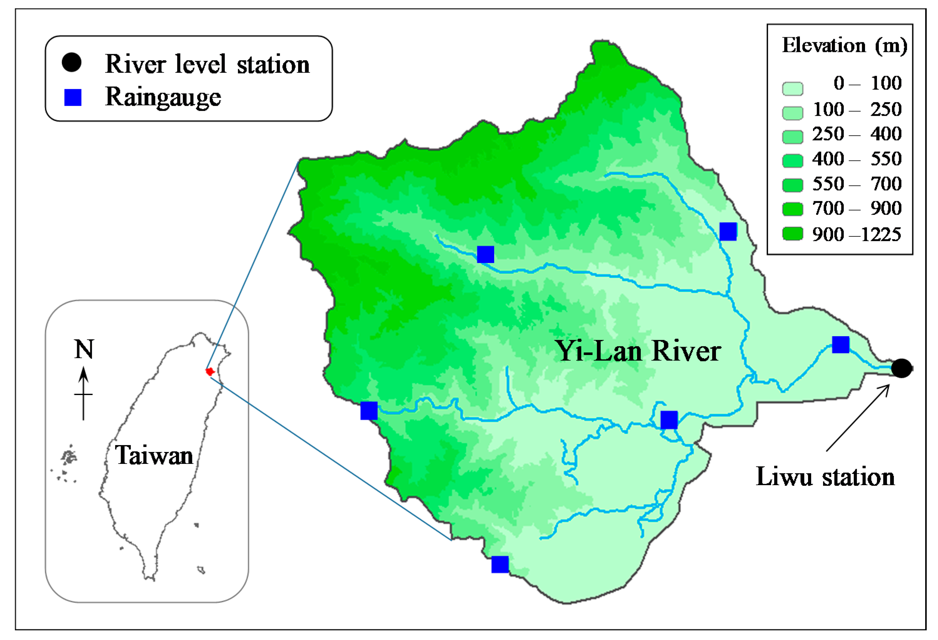
In this study, Yilan River (Figure 2) in Taiwan was selected as the study area. There are some river level stations in the Yi-Lan River basin. The Liwu station that has relatively more complete records than other stations was used in this study. Therefore, the flood stage at Liwu station was the target for real-time forecasting. The Liwu basin has an area of 108.1 km². Hourly rainfall data from six gauges and hourly river stage data at Liwu station from 2012 to 2018 were collected, and 15 flood events with complete rainfall and stage data were obtained. The collected 15 flood events were divided into a calibration set with 10 events and a validation set with 5 events.

Table 1. Collected flood events and their statistics.

Event No.	Name of Typhoon or Storm	Date	Rainfall Duration (h)	Peak Flood Stage (m)	Total Rainfall (mm)	Note
1	Jelawat	26 September 2012	96	1.22	85.2	Calibration
2	Trami	20 August 2013	71	2.14	196.3	Calibration
3	Kongrey	31 August 2013	44	1.69	138.0	Calibration
4	Usagi	20 September 2013	60	1.71	76.4	Calibration
5	Fitow	4 October 2013	67	1.62	118.5	Calibration
6	Matmo	21 July 2014	79	2.28	156.9	Calibration
7	Storm 0809	09 August 2014	133	1.22	145.6	Calibration
8	Fungwong	20 September 2014	147	2.91	364.8	Calibration
9	Dujuan	27 September 2015	86	4.23	188.2	Calibration
10	Meranti	14 September 2016	72	1.69	103.9	Calibration
11	Megi	26 September 2016	77	3.39	158.5	Validation
12	Storm 0601	1 June 2017	79	1.34	122.3	Validation
13	Storm 1013	13 October 2017	73	4.41	351.3	Validation
14	Maria	10 July 2018	41	1.47	107.4	Validation
15	Yutu	1 November 2018	73	2.52	219.9	Validation

lists the flood events with information on the source event (typhoon or storm), date of occurrence, rainfall duration, peak flood stage, and total rainfall amount. Spatially averaged rainfall was calculated from six gauges using the Thiessen polygon method, and was used as the rainfall variable in the study.

3.2. Deterministic Model Development and Forecasting

This study used SVR to perform deterministic forecasting of the flood stage at Liwu station. The observed rainfall and river stages at Liwu station during flood events were selected as input variables because of the strong relationship between these data and future stages. As the cross-sections of a river change markedly during a flood, the absolute river stage may not provide appropriate information for discriminating floods. Instead, the river stage increment, which is the river stage relative to the initial stage at the beginning of a flood event, is a more relevant variable for determining flood magnitude. Thus, the river stage increment relative to the initial stage was chosen as the stage variable for this study. Specifically, the initial stage was subtracted from the river stage data, and the obtained residual (stage increment) was the stage variable used in this study. The forecasted absolute river stage can be simply obtained by adding the forecasted stage increment to the initial stage.

Furthermore, the data of spatially averaged rainfall (R) and stage increment (S) were normalized to a range of [0, 1]. The benefit of using normalized data is avoiding one variable dominating others when the differences in their values are notable. Bray and Han [25] demonstrated that the SVR model with normalized data outperformed that without normalized data. The time lags between rainfall and stage had to be identified to construct the forecasting model; therefore, the correlation coefficients among lagged variables were calculated to identify relevant input variables for the forecasted variables [26,51]. The correlated time lags between stage and rainfall were 1–5 hours and the correlated time lags for the stage itself were 1–3 hours. Therefore, the SVR stage forecasting model in this study had eight inputs, and the model structure can be expressed as follows:

$${\widehat{S}}_{t+1}=f_{\mathrm{SVR}}\left[S_t,S_{t-1},S_{t-2},R_t,R_{t-1},R_{t-2},R_{t-3},R_{t-4}\right]$$

(13)

where $\widehat{S}$ is the forecasted flood stage; $S$ is the observed flood stage; $R$ is the observed average rainfall; $f_{\mathrm{SVR}}$ indicates the SVR model; and the subscript $t$ is the time index. The SVR model was calibrated using normalized data, and the original model outputs were the flood stages in the normalized scale. The output flood stages were transformed to their actual scale to match the observations. The SVR model, Equation (13), was established using data from 10 calibration flood events. This study used the root mean square error (RMSE) as the objective function to optimize the SVR parameters.

$$\mathrm{RMSE}=\sqrt{\frac{{{\displaystyle \sum }}_{i=1}^n{\left(S_i-{\widehat{S}}_i\right)}^2}{n}}$$

(14)

where $n$ is the number of data. During the calibration phase, the SVR model simulated flood events with an RMSE value of 0.07 m, indicating that the model was well calibrated. The SVR model, Equation (13), was used to perform real-time deterministic forecasting with a lead time of 1 hour regarding the five validation events. To perform multiple-hour-ahead forecasting, Equation (13) could be used in a recursive form as in Equations (15) and (16), where the future stage inputs ${\widehat{S}}_{t+2}$ and ${\widehat{S}}_{t+1}$ can be available from the forecasted data and the future rainfall is obtained from naïve forecasts; that is, ${\widehat{R}}_{t+2}={\widehat{R}}_{t+1}=R_t$.

$${\widehat{S}}_{t+2}=f_{\mathrm{SVR}}\left[{\widehat{S}}_{t+1},S_t,S_{t-1},{\widehat{R}}_{t+1},R_t,R_{t-1},R_{t-2},R_{t-3}\right]$$

(15)

$${\widehat{S}}_{t+3}=f_{\mathrm{SVR}}\left[{\widehat{S}}_{t+2},{\widehat{S}}_{t+1},S_t,{\widehat{R}}_{t+2},{\widehat{R}}_{t+1},R_t,R_{t-1},R_{t-2}\right]$$

(16)

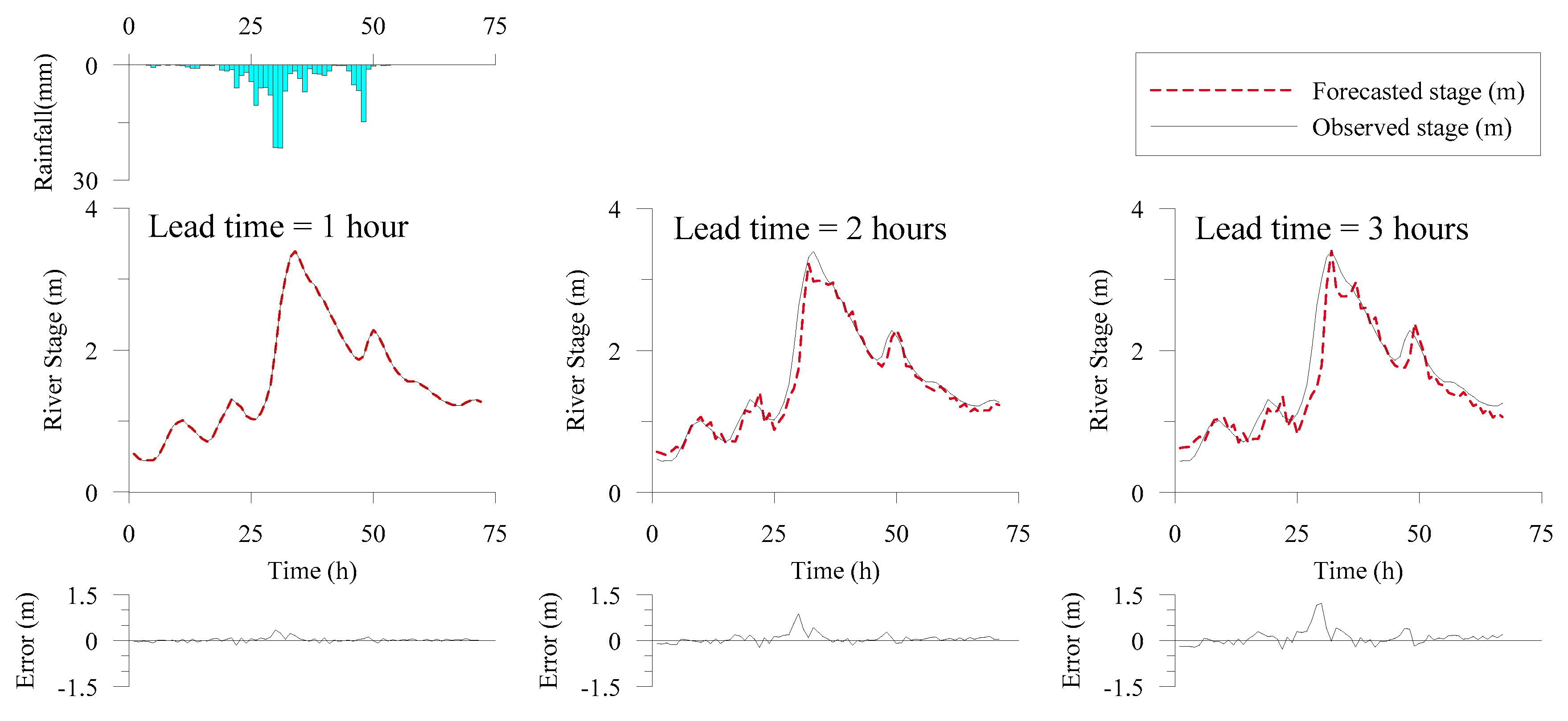
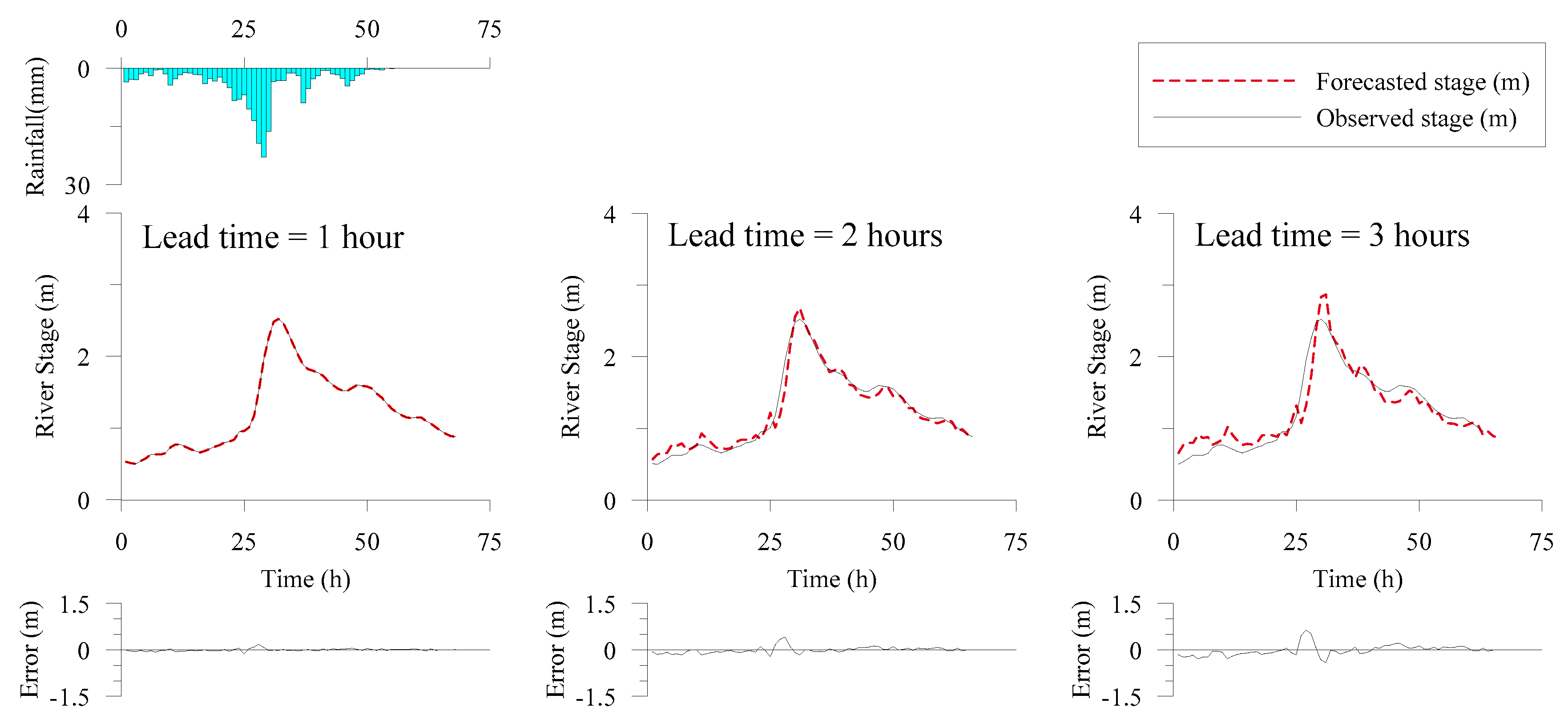
Figure 3 and Figure 4 present the deterministic forecasting results of the flood hydrographs for Events 11 and 15, respectively. Basin average rainfall and forecast error are also presented in the figures. The forecasted hydrographs were close to the observed ones and the forecast errors were small, indicating that the deterministic forecasting model could effectively perform real-time forecasting with lead times of 1–3 hours. To evaluate the forecasting performance in an objective manner, statistical indices, the RMSE, and the coefficient of efficiency (CE), were calculated with respect to validation events.

$$\mathrm{CE}=1-\frac{{{\displaystyle \sum }}_{i=1}^n{\left(S_i-{\widehat{S}}_i\right)}^2}{{{\displaystyle \sum }}_{i=1}^n{\left(S_i-\overline{S}\right)}^2}$$

(17)

where $\overline{S}$ is the average of the observation stage. The CE value being closer to unity indicated good model performance.

Table 2. Statistical indices for deterministic forecasting.

Lead Time	RMSE (m)	CE
1 hour	0.07	0.99
2 hours	0.15	0.97
3 hours	0.25	0.93

lists the statistical indices of the RMSE and CE with respect to multiple-hour-ahead forecasting for validation events. The low RMSE and high CE values confirmed that the SVR model could effectively perform deterministic forecasting.

4. Probabilistic Forecasting

4.1. Probabilistic Model Development

This section describes the use of the FIM to obtain error probability distributions. The deterministic forecasting model was originally used with normalized data. Thus, fuzzy inference was also performed with data in a normalized scale. First, the data regarding the input variables were transformed into fuzzy sets by applying a fuzzy membership function, namely the Gaussian membership function in Equation (9). The parameter of the membership function is the dispersion parameter$\sigma$. As parameter$\sigma$ indicates the dispersion of the data, adopting the standard deviation of the data as the parameter is logical. The parameters of the fuzzy membership function for rainfall (R) and stage (S) were 0.18 and 0.14, respectively, at their normalized scale.

Subsequently, the fuzzy rules were used to formulate a conditional statement to infer the forecast errors. The deterministic model used eight inputs (see those in Equation (13)) to produce the forecasts. Therefore, the forecast errors were dependent on the used inputs. Using these inputs in the premise of the fuzzy rule is rational; however, too many variables in the premise may lead to an inadequate implication. Moreover, lagged input variables can contain the same information when naïve forecasting is applied for forecasting with longer lead times. Therefore, the premise part was simplified using the most relevant variables of rainfall and stage at time $t$. That is, the variables $R_t$ and $S_t$ were used in the premise to infer the forecast errors with lead times of 1–3 hours. Accordingly, the fuzzy rule was formulated as

$$\begin{gathered} \mathrm{IF} \left(S_t\mathrm{is}{F}_s\right)\mathrm{and}\left(R_t\mathrm{is}{F}_R\right) \\ \mathrm{THEN} \left(E_{t+1}\mathrm{is}{F}_{E1}\right)\mathrm{and}\left(E_{t+2}\mathrm{is}{F}_{E2}\right)\mathrm{and}\left(E_{t+3}\mathrm{is}{F}_{E3}\right) \end{gathered}$$

(18)

where $F_s$ and $F_R$, are fuzzy sets defined by the Gaussian fuzzy membership function pertaining to variables $S_t$ and $R_t$, respectively; $E_{t+1}$, $E_{t+2}$, and $E_{t+3}$ are inferred forecast errors with lead times of 1–3 hours; and $F_{E1}$, $F_{E2}$, and $F_{E3}$ are the respective fuzzy sets of forecast errors.

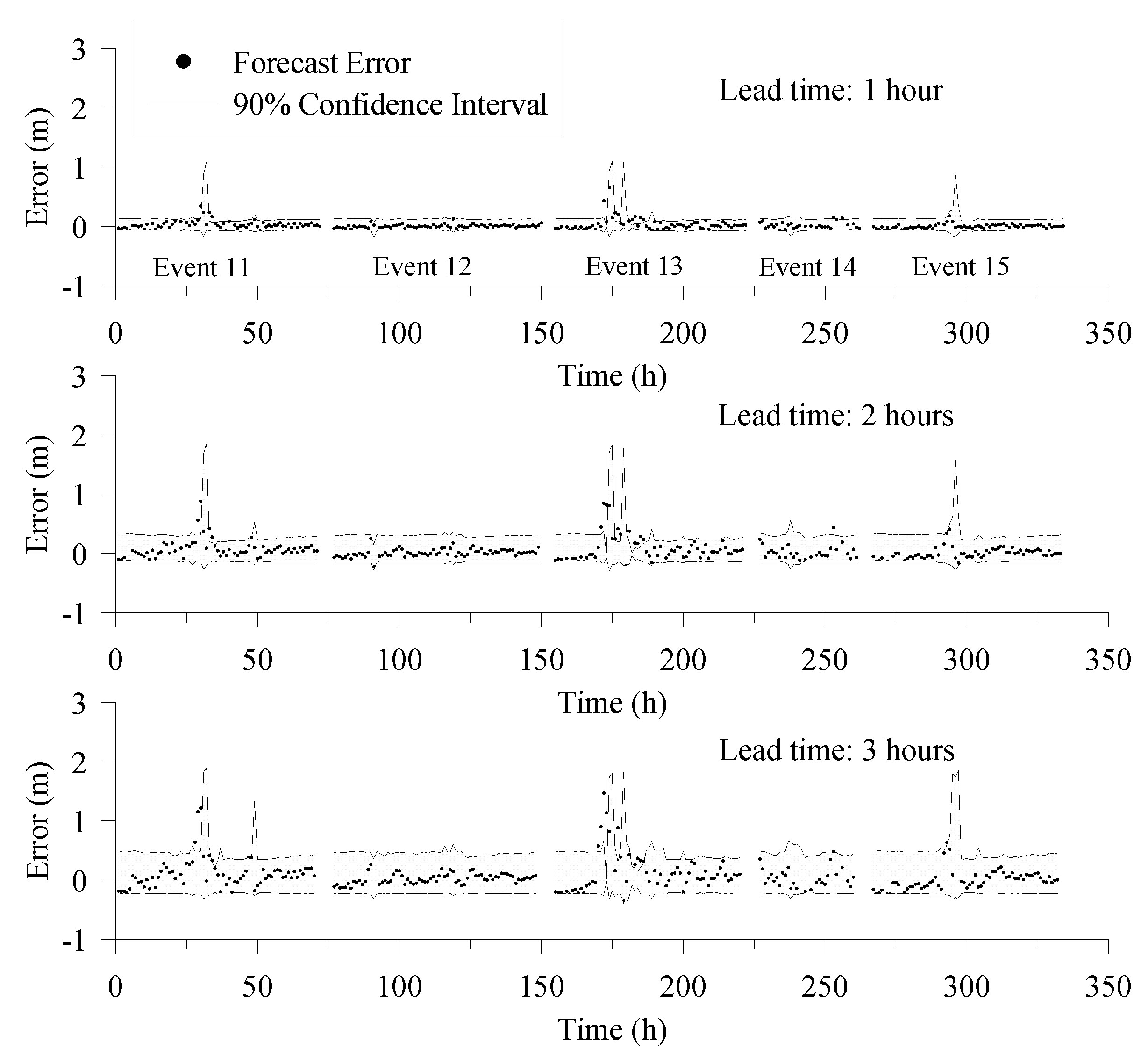
When stage and rainfall data $S_t$ and $R_t$ at present time $t$ were available, fuzzy inference could be conducted to derive the aggregated output fuzzy set. The proposed defuzzification approach was then employed to obtain the probability distributions of forecast errors. After defuzzification is performed, the derived probability distribution may demonstrate a rough-shaped curve. To solve this problem, this study applied the k-NN method to smooth the rough probability curve. The smoothing process generates numerous data to form a smooth curve to replace the original probability distribution’s rough curve. A resampling technique was adopted to implement the smoothing. At each sampling time, an object data item was randomly selected from the original probability distribution. Then, the k-NN method was applied to select three data items nearest to the object from the original probability distribution (k was set to 3 herein). The mean and standard deviation of the three data items were calculated to construct an interval, of which the upper and lower boundaries were the mean ± standard deviation, respectively. Next, a number within the interval was randomly picked to become an adjusted value to refine the probability distribution. The resampling process was repeated 10,000 times to produce a smooth probability curve with 10,000 values. With the derived smooth probability distribution, different confidence levels could be used to form the predictive confidence interval (CI). Figure 5 presents the forecast errors and the predicted 90% CI pertaining to five validation events with continuous data sequences. The confidence region could include most of the forecast errors, indicating that the CI practically covers the uncertainty of the forecast errors. The confidence region is extended with the forecast lead time, which is also rational in light of the uncertainty in forecasting.

4.2. Probabilistic Forecasting Results

The probabilistic flood-stage forecasting results were obtained by adding the probability distribution of forecast errors to the deterministic stage forecasts. Figure 6 illustrates the probabilistic flood-stage forecasting results with 90% CIs for validation events. For 1-hour forecasting, the confidence regions covered most of the observed data well with a narrow span, indicating that the proposed probabilistic forecasting method was both correct and useful. The CI range widened when the lead times increased to 2–3 hours. Moreover, the predictive CIs around the peak stage broadened sharply, and the upper boundary of the 90% CI was large. This meant that the predictive CI was less practical around the peak, because a larger CI indicates less confidence in the object of interest. Nevertheless, the proposed probabilistic forecasting model reflected the existence of greater uncertainty around the peak flood.

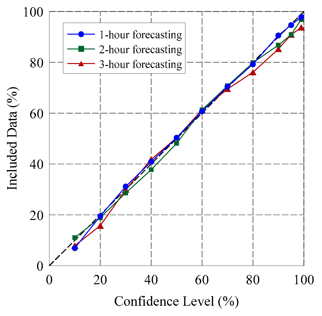
If the predictive probability distribution can effectively explain the forecasting uncertainty, then the percentage of data included in the CI will be identical to the confidence level. Therefore, the quantity of data that are correctly enclosed within the confidence region can be used as a guide to assess the probabilistic forecasting results. Figure 7 plots the percentages of observed flood stages that were included in the CI for confidence levels of 10%, 20%, …, 90%, 95%, and 99%, with respect to validation events. The percentages of included data closely matched the confidence levels, because the points on the graph were close to the 45° line. Scrutinizing the data regarding different lead times revealed that the probabilistic forecasting performance only decreased marginally with an increase in lead times. This suggested that the probabilistic forecasts with longer lead times were not inferior to those with shorter lead times in terms of this assessment measure. The capability of the proposed probabilistic forecasting model that involves using multiple machine learning methods is promising.

5. Conclusions

Probabilistic forecasts are more informative and helpful than deterministic forecasts in practical flood forecasting. This study developed a real-time probabilistic forecasting model for impending flash floods using various machine learning methods. The probabilistic forecasting method combines deterministic forecasting and the probability distribution of forecast errors. SVR was employed to provide deterministic forecasts, and an FIM with a modified scheme for defuzzification was applied to deduce the predictive probability distribution of forecast errors. A resampling scheme with the k-NN method was used to refine the predictive probability distribution. The probabilistic forecasting results could thus be presented using a CI.

The proposed methodology was applied to perform probabilistic flood-stage forecasting with lead times of 1–3 hours in Taiwan’s Yilan River. Correlation analysis was performed to determine the lagged inputs, and a recursive form of the model was established to perform multiple-hour-ahead forecasts. The SVR performed deterministic forecasting well, as was indicated by the low RMSE and high CE values. The probabilistic forecasting results were agreeable because the 90% CI could cover most of the observations with a narrow band width. To objectively assess the probabilistic forecasting performance, this study adopted a quantitative measure that calculated the percentage of observations included in the predictive CI. The percentages of included data closely matched the confidence levels, suggesting the capability of the proposed probabilistic forecasting model that involves using multiple machine learning methods.

References

- Chen, S.T.; Yu, P.S. Real-Time probabilistic forecasting of flood stages. J. Hydrol. 2007, 340, 63–77. [Google Scholar] [CrossRef]
- Krzysztofowicz, R. The case for probabilistic forecasting in hydrology. J. Hydrol. 2001, 249, 2–9. [Google Scholar] [CrossRef]
- Krzysztofowicz, R. Bayesian theory of probabilistic forecasting via deterministic hydrologic model. Water Resour. Res. 1999, 35, 2739–2750. [Google Scholar] [CrossRef] [Green Version]
- Krzysztofowicz, R. Bayesian system for probabilistic river stage forecasting. J. Hydrol. 2002, 268, 16–40. [Google Scholar] [CrossRef]
- Krzysztofowicz, R.; Maranzano, C.J. Bayesian system for probabilistic stage transition forecasting. J. Hydrol. 2004, 299, 15–44. [Google Scholar] [CrossRef]
- Biondi, D.; De Luca, D.L. Performance assessment of a Bayesian Forecasting System (BFS) for real-Time flood forecasting. J. Hydrol. 2013, 479, 51–63. [Google Scholar] [CrossRef]
- Georgakakos, K.P.; Seo, D.-J.; Gupta, H.; Schaake, J.; Butts, M.B. Towards the characterization of streamflow simulation uncertainty through multimodel ensembles. J. Hydrol. 2004, 298, 222–241. [Google Scholar] [CrossRef]
- Diomede, T.; Davolio, S.; Marsigli, C.; Miglietta, M.M.; Moscatello, A.; Papetti, P.; Tiziana Paccagnellal, T.; Andrea Buzzi, A.; Malguzzi, P. Discharge prediction based on multi-Model precipitation forecasts. Meteorol. Atmos. Phys. 2008, 101, 245–265. [Google Scholar] [CrossRef] [Green Version]
- Davolio, S.; Miglietta, M.M.; Diomede, T.; Marsigli, C.; Morgillo, A.; Moscatello, A. A meteo-Hydrological prediction system based on a multi-Model approach for precipitation forecasting. Nat. Hazard. Earth Syst. 2008, 8, 143–159. [Google Scholar] [CrossRef]
- Beven, K.J.; Binley, A. The future of distributed models: Model calibration and uncertainty prediction. Hydrol. Process. 1992, 6, 279–298. [Google Scholar] [CrossRef]
- Franks, S.W.; Gineste, P.; Beven, K.J.; Merot, P. On constraining the predictions of a distributed model: The incorporation of fuzzy estimates of saturated areas into the calibration process. Water Resour. Res. 1998, 34, 787–797. [Google Scholar] [CrossRef]
- Hunter, N.M.; Bates, P.D.; Horritt, M.S.; de Roo, A.P.J.; Werner, M.G.F. Utility of different data types for calibrating flood inundation models within a GLUE framework. Hydrol. Earth Syst. Sci. 2005, 9, 412–430. [Google Scholar] [CrossRef]
- Fan, F.M.; Collischonn, W.; Quiroz, K.J.; Sorribas, M.V.; Buarque, D.C.; Siqueira, V.A. Flood forecasting on the Tocantins River using ensemble rainfall forecasts and real-time satellite rainfall estimates. J. Flood Risk Manag. 2016, 9, 278–288. [Google Scholar] [CrossRef]
- Han, S.; Coulibaly, P. Probabilistic flood forecasting using hydrologic uncertainty processor with ensemble weather forecasts. J. Hydrometeorol. 2019, 20, 1379–1398. [Google Scholar] [CrossRef]
- Leandro, J.; Gander, A.; Beg, M.N.A.; Bhola, P.; Konnerth, I.; Willems, W.; Carvalho, R.; Disse, M. Forecasting upper and lower uncertainty bands of river flood discharges with high predictive skill. J. Hydrol. 2019, 576, 749–763. [Google Scholar] [CrossRef]
- Montanari, A.; Brath, A. A stochastic approach for assessing the uncertainty of rainfall-Runoff simulations. Water Resour. Res. 2004, 40, W01106. [Google Scholar] [CrossRef]
- Tamea, S.; Laio, F.; Ridolfi, L. Probabilistic nonlinear prediction of river flows. Water Resour. Res. 2005, 41, W09421. [Google Scholar] [CrossRef] [Green Version]
- Weerts, A.H.; Winsemius, H.C.; Verkade, J.S. Estimation of predictive hydrological uncertainty using quantile regression: Examples from the National Flood Forecasting System (England and Wales). Hydrol. Earth Syst. Sci. 2011, 15, 255–265. [Google Scholar] [CrossRef] [Green Version]
- Teschl, R.; Randeu, W.L.; Teschl, F. Improving weather radar estimates of rainfall using feed-Forward neural networks. Neural Netw. 2007, 20, 519–527. [Google Scholar] [CrossRef]
- Chen, S.T.; Yu, P.S.; Liu, B.W. Comparison of neural network architectures and inputs for radar rainfall adjustment for typhoon events. J. Hydrol. 2011, 405, 150–160. [Google Scholar] [CrossRef]
- Chang, F.J.; Chiang, Y.M.; Chang, L.C. Multi-Step-Ahead neural networks for flood forecasting. Hydrolog. Sci. J. 2007, 52, 114–130. [Google Scholar] [CrossRef]
- Jhong, Y.D.; Chen, C.S.; Lin, H.P.; Chen, S.T. Physical hybrid neural network model to forecast typhoon floods. Water 2018, 10, 632. [Google Scholar] [CrossRef] [Green Version]
- Lin, G.F.; Wu, M.C. An RBF network with a two-Step learning algorithm for developing a reservoir inflow forecasting model. J. Hydrol. 2011, 405, 439–450. [Google Scholar] [CrossRef]
- Sattari, M.T.; Yurekli, K.; Pal, M. Performance evaluation of artificial neural network approaches in forecasting reservoir inflow. Appl. Math. Model. 2012, 36, 2649–2657. [Google Scholar] [CrossRef]
- Bray, M.; Han, D. Identification of support vector machines for runoff modelling. J. Hydroinform. 2004, 6, 265–280. [Google Scholar] [CrossRef] [Green Version]
- Yu, P.S.; Chen, S.T.; Chang, I.F. Support vector regression for real-time flood stage forecasting. J. Hydrol. 2006, 328, 704–716. [Google Scholar] [CrossRef]
- Lin, G.F.; Chou, Y.C.; Wu, M.C. Typhoon flood forecasting using integrated two-Stage support vector machine approach. J. Hydrol. 2013, 486, 334–342. [Google Scholar] [CrossRef]
- Chen, S.T.; Yu, P.S.; Tang, Y.H. Statistical downscaling of daily precipitation using support vector machines and multivariate analysis. J. Hydrol. 2010, 385, 13–22. [Google Scholar] [CrossRef]
- Yang, T.C.; Yu, P.S.; Wei, C.M.; Chen, S.T. Projection of climate change for daily precipitation: A case study in Shih-Men Reservoir catchment in Taiwan. Hydrol. Process. 2011, 25, 1342–1354. [Google Scholar] [CrossRef]
- Chen, S.T.; Yu, P.S. Pruning of support vector networks on flood forecasting. J. Hydrol. 2007, 347, 67–78. [Google Scholar] [CrossRef]
- Chen, S.T. Mining informative hydrologic data by using support vector machines and elucidating mined data according to information entropy. Entropy 2015, 17, 1023–1041. [Google Scholar] [CrossRef] [Green Version]
- Lin, G.F.; Chen, G.R.; Wu, M.C.; Chou, Y.C. Effective forecasting of hourly typhoon rainfall using support vector machines. Water Resour. Res. 2009, 45. [Google Scholar] [CrossRef]
- Chen, S.T. Multiclass support vector classification to estimate typhoon rainfall distribution. Disaster Adv. 2013, 6, 110–121. [Google Scholar]
- Yu, P.S.; Chen, S.T.; Wu, C.C.; Lin, S.C. Comparison of grey and phase-Space rainfall forecasting models using fuzzy decision method. Hydrolog. Sci. J. 2004, 49, 655–672. [Google Scholar] [CrossRef]
- Yu, P.S.; Chen, S.T.; Chen, C.J.; Yang, T.C. The potential of fuzzy multi-Objective model for rainfall forecasting from typhoons. Nat. Hazards 2005, 34, 131–150. [Google Scholar] [CrossRef]
- Alvisi, S.; Mascellani, G.; Franchini, M.; Bardossy, A. Water level forecasting through fuzzy logic and artificial neural network approaches. Hydrol. Earth Syst. Sci. 2006, 10, 1–17. [Google Scholar] [CrossRef] [Green Version]
- Chen, C.S.; Jhong, Y.D.; Wu, T.Y.; Chen, S.T. Typhoon event-Based evolutionary fuzzy inference model for flood stage forecasting. J. Hydrol. 2013, 490, 134–143. [Google Scholar] [CrossRef]
- Wolfs, V.; Willems, P. A data driven approach using Takagi-Sugeno models for computationally efficient lumped floodplain modeling. J. Hydrol. 2013, 503, 222–232. [Google Scholar] [CrossRef]
- Lohani, A.K.; Goel, N.K.; Bhatia, K.K.S. Improving real time flood forecasting using fuzzy inference system. J. Hydrol. 2014, 509, 25–41. [Google Scholar] [CrossRef]
- Chen, C.S.; Jhong, Y.D.; Wu, W.Z.; Chen, S.T. Fuzzy time series for real-time flood forecasting. Stoch. Env. Res. Risk A 2019, 33, 645–656. [Google Scholar] [CrossRef]
- Toth, E.; Brath, A.; Montanari, A. Comparison of short-Term rainfall prediction models for real-Time flood forecasting. J. Hydrol. 2000, 239, 132–147. [Google Scholar] [CrossRef]
- Coulibaly, P.; Haché, M.; Fortin, V.; Bobée, B. Improving daily reservoir inflow forecasts with model combination. J. Hydrol. Eng. 2005, 10, 91–99. [Google Scholar] [CrossRef]
- Sharif, M.; Burn, D.H. Simulating climate change scenarios using an improved k-nearest neighbor model. J. Hydrol. 2006, 325, 179–196. [Google Scholar] [CrossRef]
- Sapin, J.; Rajagopalan, B.; Saito, L.; Caldwell, R.J. A k-Nearest neighbor based stochastic multisite flow and stream temperature generation technique. Environ. Modell. Softw. 2017, 91, 87–94. [Google Scholar] [CrossRef]
- Vapnik, V.N. The Nature of Statistical Learning Theory; Springer: New York, NY, USA, 1995. [Google Scholar]
- Vapnik, V.N. Statistical Learning Theory; Wiley: New York, NY, USA, 1998. [Google Scholar]
- Reddy, C.S.; Raju, K.V.S.N. An improved fuzzy approach for COCOMO’s effort estimation using Gaussian membership function. J. Softw. 2009, 4, 452–459. [Google Scholar] [CrossRef]
- Yu, P.S.; Chen, S.T. Updating real-Time flood forecasting using a fuzzy rule-Based model. Hydrolog. Sci. J. 2005, 50, 265–278. [Google Scholar] [CrossRef]
- Chen, S.T. Probabilistic forecasting of coastal wave height during typhoon warning period using machine learning methods. J. Hydroinform. 2019, 21, 343–358. [Google Scholar] [CrossRef]
- Filev, D.; Yager, R.R. A generalized defuzzification method via BAD distributions. Int. J. Intell. Syst. 1991, 6, 687–697. [Google Scholar] [CrossRef]
- Solomatine, D.P.; Dulal, K.N. Model trees as an alternative to neural networks in rainfall-Runoff modelling. Hydrolog. Sci. J. 2003, 48, 399–411. [Google Scholar] [CrossRef]
Figure 1.
Fuzzy inference process.
Figure 2.
Yilan River basin and stations.
Figure 3.
Deterministic forecasting results (Event 11).
Figure 4.
Deterministic forecasting results (Event 15).
Figure 5.
Forecast errors and 90% confidence intervals.
Figure 6.
Probabilistic forecasting with 90% confidence intervals.
Figure 7.
Percentage of observed data included in the confidence region.