Bed-Sediment Transport Conditions along the Sagavanirktok River in Northern Alaska, USA


Water and Environmental Research Center, University of Alaska Fairbanks, Fairbanks, AK 99775, USA
Water 2020, 12(3), 774; https://doi.org/10.3390/w12030774
Submission received: 13 December 2019
/
Revised: 20 February 2020
/
Accepted: 8 March 2020
/
Published: 11 March 2020
(This article belongs to the Section Hydraulics and Hydrodynamics)
Abstract
:This manuscript presents a study in predicting bed-sediment transport rates along the Sagavanirktok River in Alaska. Extensive field activities took place to accomplish this goal: four hydro-meteorological stations were installed in a 150 km reach along the river in summer 2015. During the same year, pits were excavated near the stations, and in subsequent summers, the pits were surveyed multiple times in conjunction with taking discharge measurements. Water slope was measured and bed sediment was characterized. Site-specific relationships between water levels and cross-section water depths were developed. Volume change between consecutive surveys was calculated, and main flood events between surveys were identified. Finally, the first bed-sediment transport equations valid for the Sagavanirktok River were developed. Considering the intrinsic error in sediment transport predictions, the agreement between predicted and measured sediment transport values is good. These equations could be used by resource managers when predicting the expected time for an excavated material site in the Sagavanirktok River to refill.
1. Introduction
In general, Alaska—the northernmost state in the U.S.—is characterized by extreme cold weather, vast uninhabited areas, and sparse hydro-meteorological data. The lack of data is especially pronounced in aspects related to sediment transport processes in rivers. Efforts to develop new data sets and to improve our knowledge of arctic rivers are usually carried out in response to natural disasters.
A multiyear hydro-sedimentological study of an area along an approximately 150 km reach on the Sagavanirktok River was performed in response to an unprecedented flood event that occurred during spring 2015, when the river overtopped and severely damaged the Dalton Highway near Deadhorse, an oil-support town located in northern Alaska [1]. The Dalton Highway, which provides the only terrestrial access to Deadhorse, parallels the Sagavanirktok River along the study area (Figure 1). Immediately after the flood, the Alaska Department of Transportation and Public Facilities (ADOT&PF) began work on a project to raise the highway. The road improvement work required a substantial amount of material, which in this remote location of Alaska was acquired by extracting sediment from the river. Questions about the sediment replenishment rates were raised by resource managers, but data on Sagavanirktok River bed-sediment transport rates were nonexistent. The hydro-sedimentological study discussed here was conducted to fill the information gap.
This manuscript presents field activities and analysis performed to develop the first set of bed-sediment transport equations for the Sagavanirktok River.
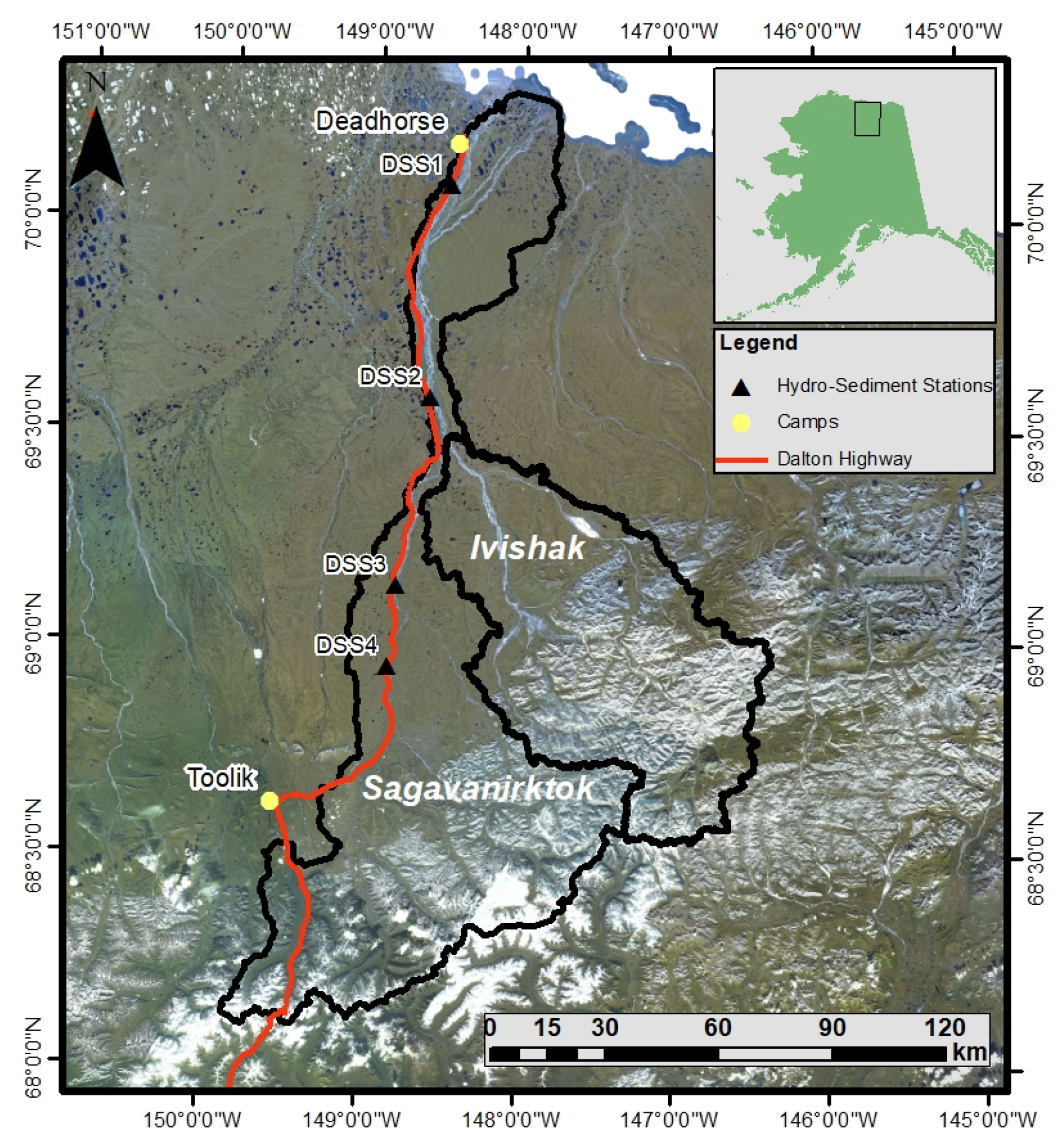
2. Geographic Location
The Sagavanirktok River flows north, from the Brooks Range to the Beaufort Sea. The river is parallel to the Dalton Highway for approximately 160 km [1]. The Sagavanirktok River basin has three distinct areas, characterized by increasing slopes: the coastal plain, foothills, and mountain region [2]. The total watershed area is roughly 13,500 km2, with two sub-basins in the mountain region: the Upper Sagavanirktok, 6500 km2, and the Ivishak, 5200 km2 [1]. Figure 1 shows the watershed boundaries as well as the Dalton Highway.
3. Methodology and Analysis
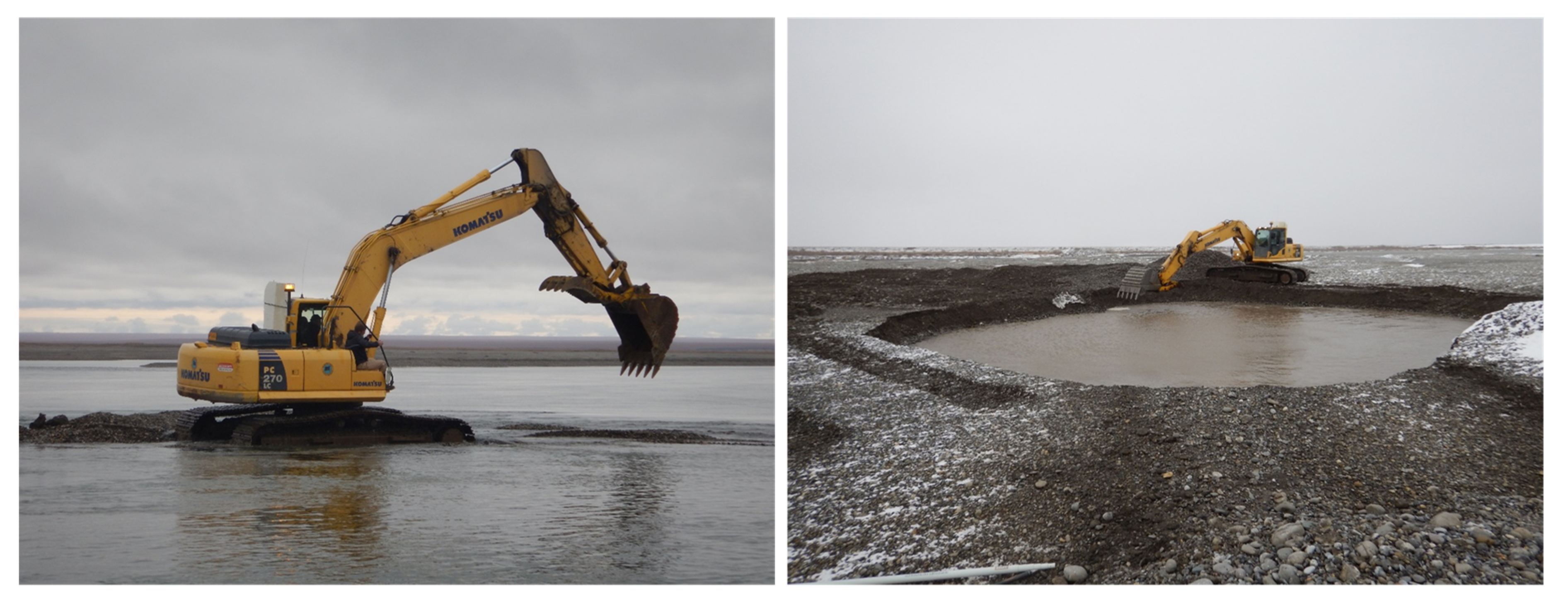
Given the location (far from population centers) and the characteristics of the study reach (limited river access), commonly used methodologies in bed-sediment transport research, such as Helley-Smith type samplers and tracers, could not be applied in this study. Seven pits dug in the river bed (Figure 2) were used as study sites in this effort to quantify bed-sediment transport rates in the Sagavanirktok River. Hydrological data (nearly continuous water levels and discrete discharge measurements) were collected in the vicinity of the pits. The pits were excavated in fall 2015 at four locations in the Sagavanirktok River channel and active floodplain (near the Dalton Highway at MP [milepost] 405 [DSS1], downstream of the Ivishak River confluence [DSS2], at Happy Valley [DSS3], and near MP318 [DSS4]). Sediment extracted from the pits was spread over the adjacent river bed. No significant changes in local topography were made. The pits were 2–3 m in depth and 8–18 m in the direction perpendicular to the flow. ADOT&PF excavated two pits at DSS2, DSS3, and DSS4, and excavated only one pit at the west channel near DSS1 [3]. The pits are referred to as wet and dry because of where they were excavated. Wet pits were excavated in water near the edge of the active channel; dry pits were excavated at gravel bars farther away from the main channel [4]. In a literature search, no reports of similar studies on rivers in arctic regions were found.
Following excavation of the pits, the sites were surveyed using a real-time kinematic (RTK) GPS, and the bathymetry was recorded using an acoustic Doppler current profiler (ADCP) or an echo sounder. The equipment used achieves horizontal and vertical accuracies of 0.7 m and 0.01 m, respectively. Beginning in June 2016, the pits were resurveyed at approximately 1-month intervals throughout the summer (3 surveys per season) to monitor volume changes. Table 1 presents the date of each bathymetric survey of the pits. On numerous occasions, bathymetric surveys in the wet pit could not be conducted because neither a motorboat nor kayak could be launched safely with the survey equipment during high water events [3]. Topo-bathymetric maps were generated after each survey, and the volume of each pit was calculated. Water slopes were measured over a 2–5 km reach using the GPS equipment (each pit was located near the middle of this distance) on both margins of the river.
To track the water level changes, vented pressure transducers were installed in the river bed at the hydrological stations, near the pits. These sensors were set to record data every 15 min. Collected data were transmitted via a complex telemetry system from each of the sites (DSS1 to DSS4 in Figure 1) in near-real-time and reported online [4].
Discharge measurements were carried out near the stations when the pits were dug and, on average, every month during summers 2016–2018. These measurements were coincident with the pit surveys. An ADCP and a GPS were mounted on a kayak or motorboat. The measurements paired with the respective water levels were used to develop rating curves for each station [3]. Average geometric dimensions (width and depth) of river cross-sections were extracted from the ADCP-generated data files. The geometric data were used to generate empirical relationships at each site (DSS1–DSS4) to estimate average water depth on the main river channel. Details on these relationships are provided in the following paragraphs.
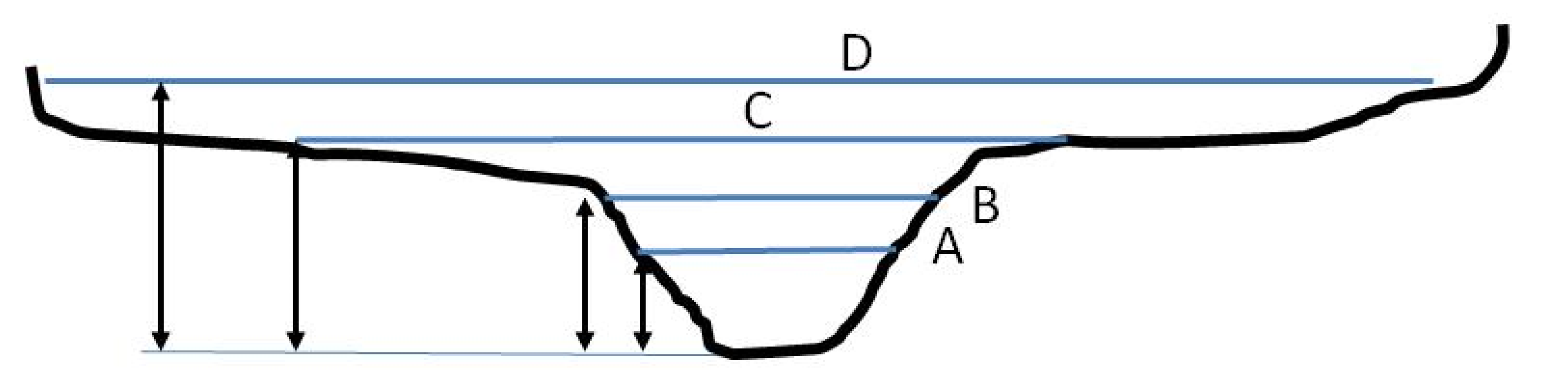
Figure 3 shows a schematic of an entire river cross-section with a main channel. In the figure, it is possible to see that at low or medium flows, all discharge measurements will be done inside the main channel. At higher water levels (lines C and D in the figure), the channel width increases significantly. Thus, the average water depth over the cross-section decreases. However, it is water depth in the main channel, which is needed for calculating basic sediment transport parameters, that is of interest.
Basic summary data collected by the ADCP during a given discharge measurement (i.e., channel width and average depth) and the corresponding gauge height for each summer measurement were plotted to estimate the average water depth at bankfull condition in the main channel.
The calculation of bed shear stress, , is given by the following equation:
where γ is the specific gravity of water, H is the average water depth, and S is the water slope. Water depths in the main channel were determined by adding the extra layer of water (above bankfull) to the depth corresponding to bankfull conditions in the main channel.
Shields [5] pioneered research, involving dimensional analysis and laboratory experiments, on the threshold of motion of non-cohesive bed-sediment particles. He defined a dimensionless parameter, the Shields number, τ*, as
where ρ is the density of water, R is the submerged specific gravity of natural sediments (R = 1.65 for quartz), g is gravity, and D is the sediment diameter.
Shields determined that a minimum value is needed to initiate the motion of particles. This value is known as the critical Shields number, τc*, which ranges from 0.03 to 0.06 for gravel-bed rivers, as reported in the published literature [6]. This variation in τc* imposes an additional complication when developing a bed-sediment transport equation. A common value used in several sediment transport equations is 0.047 [6]. Wilcock et al. [7] suggested a value of 0.03 for rivers with coarse sediments, similar to the Sagavanirktok River.
Common, single-size, bed-sediment transport equations take the following general form,
where is the dimensionless sediment transport rate per unit width, which is defined as
where (Equation (3)) is a constant coefficient, which is different for various published equations; for instance, 8 Meyer-Peter and Muller [8], 5.7 Fernandez Luque and Van Beek [9], 3.97 Wong and Parker [10], and where qs (Equation (4)) is the bed load transport rate per unit width.
Furthermore, the total bed load transport rate, Qs, can be calculated as
where B is the channel width.
To estimate bed-sediment transport at each site (DSS1–DSS4) between bathymetric surveys from the river’s hydraulic conditions, the hydrographs between surveys were analyzed. After identifying the major event(s) between surveys (Figure 4), the hydrographs were simplified, retaining the key inflection points, and the relative time between these points was recorded (see Figure 5 as an example). The average water depths for each of the points were then calculated using the empirical relationships previously described.
To investigate if any of the commonly used, and simplistic, bed-sediment transport equations predicted the sediment transport estimated from successive pit surveys in the field, Laurio [11], applied several single-size bed-sediment transport equations to the Sagavanirktok River. The equations used in Laurio’s work were Meyer-Peter and Muller [8], Wong and Parker [10], Ashida and Michiue [12], Fernandez Luque and Van Beek [9], Engelund and Fredsoe [13], Lajeunesse et al. [14], Wilson [15], Parker fit to Einstein [16], as well as ACRONYM [17], software which is capable of estimating bed-sediment transport for a given grain-size distribution and is freely available. Laurio [11], concluded that none of the sediment transport equations applied successfully reproduced the sediment transport estimated from successive pit surveys in the field.
Consequently, the development of an equation capable of reproducing the data collected in the field for the Sagavanirktok River was needed. A simple structure similar to that of Equation (3) was thought to accomplish this task. Two main challenges were encountered during the development of such an equation: finding the correct value and defining the value in Equation (3). The methodologies used to define the and values are discussed in the following paragraphs.
As mentioned, one of the key components in the process was selection of the τc* value. To accomplish this task, the maximum sediment size that could be moved during the largest annual summer hydrological event (i.e., annual maximum water level elevation) was estimated in the Sagavanirktok River for the years 2016, 2017, and 2018. The analysis was not conducted for the spring breakup period because anchor ice and frozen streambed often prohibit the movement of sediment during much of breakup.
The average water depth in the main channel, corresponding to the annual maximum water level elevation, was estimated from the empirical relationships derived from all summer discharge measurements available at each site. The information collected in the field was used to calculate an average slope (the slopes on both margins were averaged). A set of different τc* values was used in combination with the maximum shear stress value, calculated from Equation (1), to estimate the maximum sediment diameter that could be moved by the river using Equation (2). These values were then compared with grain-size distributions collected in the field.
After the correct τc* value was selected, a computer program was written to find the α value in Equation (3), the second challenge in developing the bed-sediment transport equations for the Sagavanirktok River.
4. Results
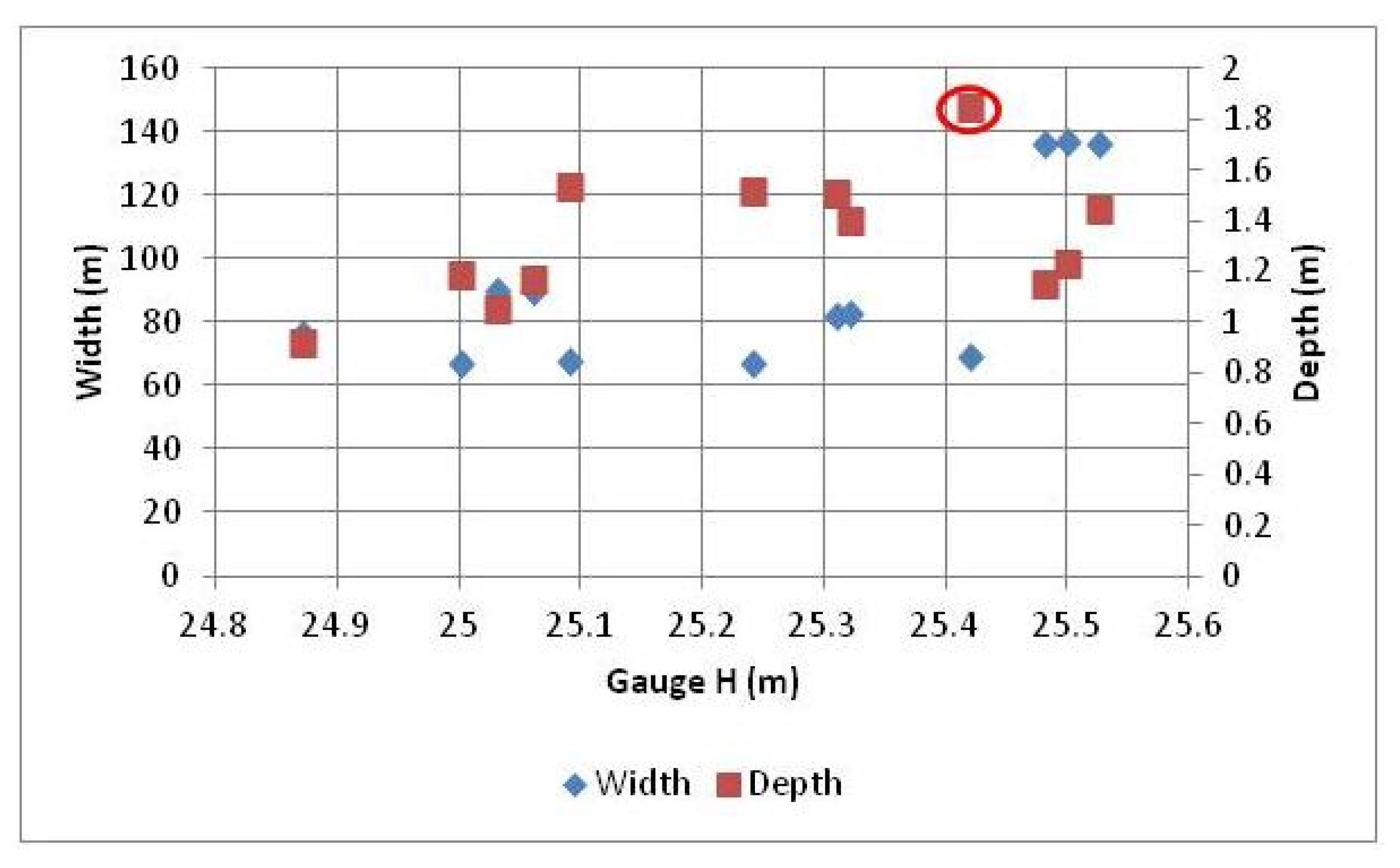
Figure 6 shows the plot of channel width and average water depth as a function of gauge height above mean sea level (AMSL) for the station at MP405 (DSS1). An inspection of the data in the figure indicates that water depths increased with increasing gauge height to about 25.42 m AMSL, while the channel width remained relatively constant. At gauge heights above 25.42 m AMLS, the average water depth decreased, and the channel width increased significantly. Consequently, the channel is considered at bankfull with a gauge height of 25.42 m AMSL (the red oval in the figure indicates the water depth that is considered bankfull depth at the main channel). The water depths corresponding to bankfull conditions for other stations were determined similarly.
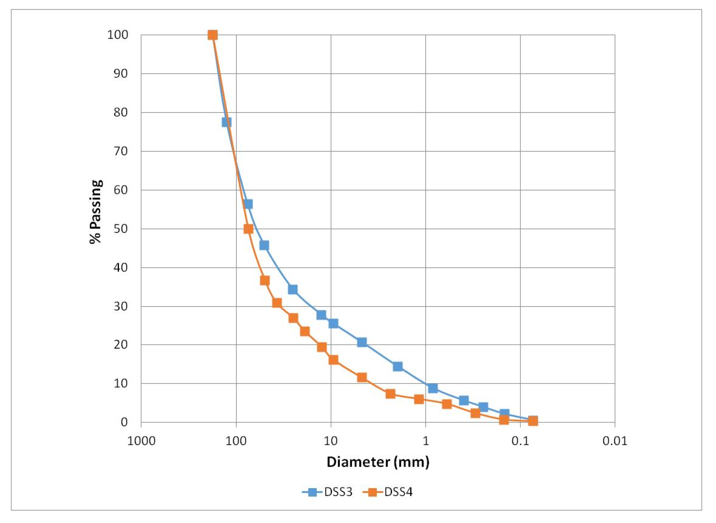
Maximum annual summer water level elevations at each station were used to calculate maximum sediment size that could be moved along the main channel. In the calculations, water slope was considered constant at each station (S = 0.0012 at DSS1; S = 0.0022 at DSS2; S = 0.0032 at DSS3; S = 0.0032 at DSS4). Some could maintain that the selection of a constant slope poses a limitation to the analysis; however, it is argued that the approach used here is reasonable, given the field logistical constraints. In addition, similar approaches have been reported in the literature [6,7]. The critical Shields number, τc*, was set to 0.03. The slope at DSS1 is close to 0.00135, reported in an early geological study conducted near Prudhoe Bay [18]. Table 2 and Table 3 provide the maximum sediment diameter at stations DSS3 and DSS4 along the Sagavanirktok River. These maximum diameters were compared with surface sediment randomly extracted from the pits during the 2018/19 winter. The maximum sediment diameters (i.e., b axis of pebbles) from the pits were 0.12 m and 0.15 m for DSS3 and DSS4, respectively. The agreement between maximum sampled sediment and maximum calculated sediment was remarkable. Grain size distributions upstream of the pits at DSS3 and DSS4 are shown in Figure 7.
Table 4 shows the volume change between consecutive surveys. From the water level data, major hydrographs were identified between the surveys. Water depths in the channel were estimated based on the empirical relationships developed for each station (see Figure 6 for instance).
A computer program was developed to identify the best alpha value that matched the sediment deposited in each pit. The representative diameter, D50, of grain-size distribution at each site was 0.03 m, 0.03 m, 0.06 m, 0.075 m for DSS1, DSS2, DSS3, and DSS4, respectively. The pit width perpendicular to flow direction was 16.5 m (DSS1), 12.5 m (DSS2 wet), 17 m (DSS2 dry), 9.5 m (DSS3 wet), 9 m (DSS3 dry), 8.5 m (DSS4 wet), and 8.5 m (DSS4 dry). A porosity of 0.4 was used in the calculations. Table 5 shows the range and average alpha values for each station, as well as the average error in the sediment deposit volume (last column in Table 5). Thus, one can conclude that the developed equations adequately reproduce the bed-sediment transport conditions along the study sites.
5. Discussion
Table 4 shows that there was appreciable sedimentation only in a few surveys, while Figure 4, which represents an example of the stations, shows that sedimentation did not occur even with similar water levels.
These facts manifest the importance of bed armoring in sediment transport processes in gravel-bed rivers. Bed armoring is defined as a coarse surface layer on the river bed, which protects the finer sediments located in the substrate from being entrained in the current [19,20,21]. Two types of armoring layers are recognized in the literature: static armoring and dynamic armoring. Static armoring develops as a result of a long period of flows over a sediment mixture constituted by coarse and fine sediments (for instance, gravel and sand). The shear stresses generated by the flows are smaller than that needed to move the largest particle but are large enough to entrain the fines. Over time, the fine sediment is winnowed from the bed surface [19]. Sediment transport in a developed static armored layer can be zero or negligible [22]. Consequently, when the sediment transport of a gravel bed is estimated from the grain-size distribution of the bed surface without considering the surface structure, the results often over-predict the transport rates [23]. In addition, it is important to re-emphasize that previously reported alpha values [8,9,10] were obtained considering uniform grain-size distributions. Consequently, armoring was not present in the derivations of those alpha coefficients. One could argue that the small alpha values obtained for the Sagavanirktok River (Table 5) intrinsically account for bed armoring, which was reported in an area near Prudhoe Bay [18].
The armor layer can break during the rising limb of high flow events, which creates a sudden increase in the sediment transport rate and will re-develop during the falling limb of these events [19]. Dynamic armoring is formed when the shear stresses are big enough to move all the particles present in the river bed. The dynamic armoring is insensitive to additional changes in the flow conditions [22].
The prediction of armoring breakup is still a challenging task because our current knowledge on the subject is somewhat limited [24]. Available literature on armoring also indicates that lift is as important as shear stress when estimating a particle’s threshold condition. Key factors in dynamic lift include the ramping duration and the ramping rate, as well as the total increase in discharge [25].
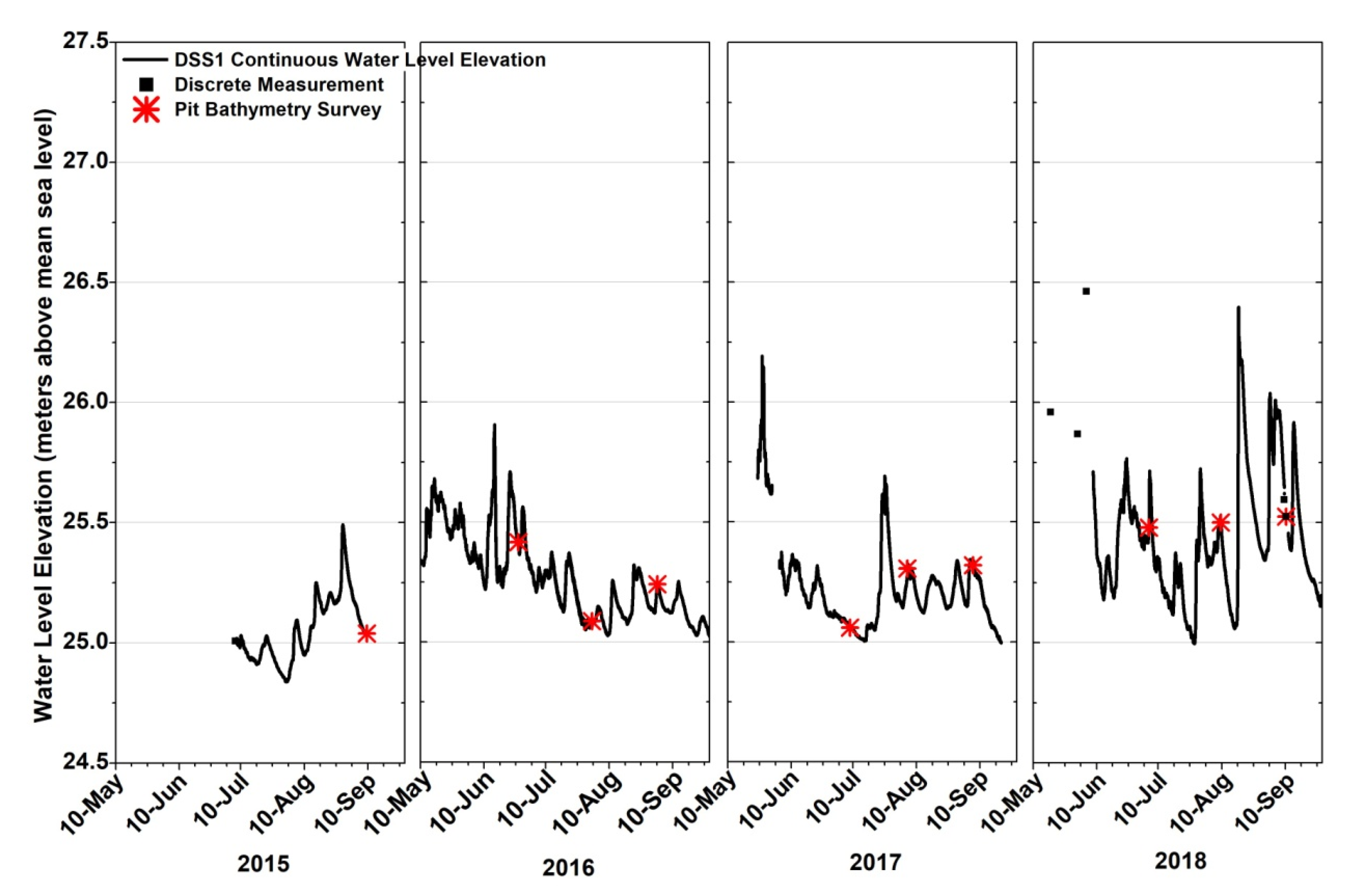
It is speculated here that spring breakup characteristics (fast vs. slow) play a fundamental role in maintaining or destroying the armored layer. In this work, fast spring breakup is defined as a process characterized by a quick increase in water depth, where the bottom ice is lifted by the mechanical action of flowing water. Under these circumstances, the ice will lift the bottom sediment attached to it and the armored layer will be destroyed. A slow spring breakup is characterized by a gradual increase in water depth. The bottom ice decays gradually in place. Consequently, the armored layer is not destroyed. This is the reason why summer events with similar water elevations produce or do not produce sediment transport. Additionally, if summer events are not strong enough to destroy the armored layer, no sedimentation inside the pits should be expected. See for instance, the main event during summer 2017 (shown in Figure 4).
The work reported here consisted of developing a set of simple equations capable of estimating bed-sediment transport rates along the Sagavanirktok River. However, an issue related to the research approach was raised during the review process. This issue is addressed below in the context of replies to rhetorical comments.
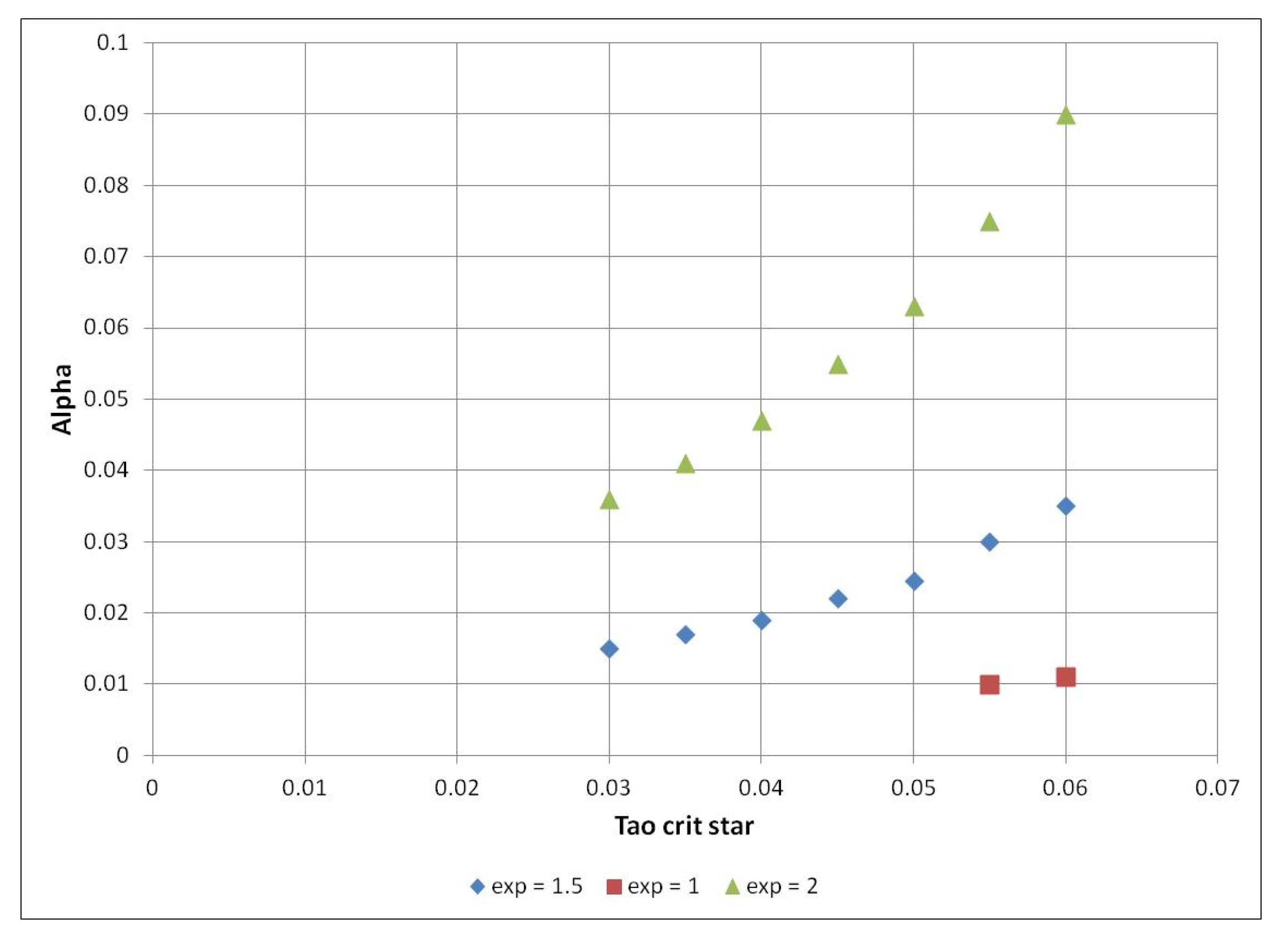
Because of the rough approximations (constant slope, use of one particle size, ignoring mixed bed material etc.) used to build the model, at least a sensitivity analysis of the parameters (critical Shields number and exponent) would have been justified. Even though the exponent in Equation (3) is fixed (1.5) in equations with similar structure, and the commonly reported value for τc* in gravel-bed rivers is 0.03, a sensitivity analysis of these two parameters was performed. Figure 8 shows the alpha values required to match a measured sediment deposit at DSS2. The results indicate that the alpha values are small, even when the τc* is doubled and the exponent is increased.
6. Conclusions
Information gathered from extensive fieldwork on the Sagavanirktok River, which included installation of several hydrological stations, multiple discharge measurements, bed-sediment characterization, water slope measurements, and multi-year topo-bathymetric surveys, was used to establish relationships between water levels AMSL and water depths in the river channel at each study site.
A value of τc* = 0.03 for the Sagavanirktok River was defined after computing the shear stress conditions and comparing maximum sediment diameters that could be moved under those hydraulic conditions, with maximum diameters found inside the pits. The agreement between calculated and field diameters is remarkable.
A computer program was developed to find the best alpha value (Equation (3)) that reproduces the bed-sediment conditions for all the study sites (DSS1–DSS4). Consequently, a basic bed-sediment transport equation for each site was defined. The calculated average errors between measured and calculated sediment volumes are relatively small, which indicates the strength of the developed equations. When comparing the alpha values with reported values in similar types of equations (Equation (3)) obtained considering uniform sediments, it is found that the alpha values for the Sagavanirktok River are smaller than the published values. It is argued here that the newly reported values account for bed armoring conditions in the channel. Because the degree of armoring varies widely from stream to stream [7], caution is recommended when applying the equations to other rivers.
Resource managers could use these equations as a rough and first-order estimation of expected time to refill of material sites excavated in the Sagavanirktok River. In a broader application, the methodology developed in this study could be applied to other rivers located in extreme cold environments, which, in general, are characterized by limited accessibility.
Funding
This work is part of the Sagavanirktok hydro-sedimentological study, which is funded by the Alaska Department of Transportation and Public Facilities, under grant #ADN2572616 to the University of Alaska Fairbanks.
Acknowledgments
The author expressly acknowledges the following UAF project team personnel, given in alphabetical order: Joel Bailey, Allen Bondurant, Joel Homan, John Keech, Isaac Ladines, Eric LaMesjerant, Jenah Laurio, Ravi Paturi, Kathy Petersen, Emily Youcha, and Dragos Vas. All of them participated in data collection and/or data processing efforts. Without their efforts, this manuscript would not be possible.
Conflicts of Interest
The author declares no conflict of interest.
References
- Toniolo, H.; Stutzke, J.; Lai, A.; Youcha, E.; Tschetter, T.; Vas, D.; Keech, J.; Irving, K. Antecedent conditions and damage caused by 2015 spring flooding on the Sagavanirktok River, Alaska. J. Cold Reg. Eng. 2017, 31, 05017001. [Google Scholar] [CrossRef]
- Kane, D.L.; Youcha, E.K.; Stuefer, S.L.; Myerchin-Tape, G.; Lamb, E.; Homan, J.W.; Gieck, R.E.; Schnabel, W.E.; Toniolo, H. Hydrology and Meteorology of the Central Alaskan Arctic: Data Collection and Analysis; Report INE/WERC 14.05; Final Report; University of Alaska Fairbanks, Water and Environmental Research Center: Fairbanks, AK, USA, 2014. [Google Scholar]
- Toniolo, H.; Youcha, E.K.; Tape, K.D.; Paturi, R.; Homan, J.; Boudurant, A.; LaMesjerant, E.; Landes, I.; Vas, D.; Keech, J.; et al. Hydrological, Sedimentological, and Meteorological Observations and Analysis on the Sagavanirktok River; Report INE/WERC 18.16; Technical Report; University of Alaska Fairbanks, Institute of Northern Engineering: Fairbanks, AK, USA, 2018. [Google Scholar]
- Toniolo, H.; Youcha, E.K.; Tape, K.D.; Paturi, R.; Homan, J.; Bondurant, A.; Ladines, I.; Laurio, J.; Vas, D.; Keech, J.; et al. Hydrological, Sedimentological, and Meteorological Observations and Analysis on the Sagavanirktok River; Report INE/WERC 17.18; Interim Report; University of Alaska Fairbanks, Water and Environmental Research Center: Fairbanks, AK, USA, 2017. [Google Scholar]
- Shields, I.-A. Anwendung der Ahnlichkeitmechanik und der Turbulenzforschung auf die Gescheibebewegung; Preussischen Versuchsanstalt für Wasserbau: Berlin, Germany, 1936. [Google Scholar]
- ASCE. Sedimentation Engineering: Processes, Measurements, Modeling and Practice; Garcia, M., Ed.; ASCE: Preston, VA, USA, 2008; 1132p. [Google Scholar]
- Wilcock, P.; Pitlick, J.; Cui, Y. Sediment transport primer: Estimating bed-material transport in gravel-bed rivers. Gen. Tech. Rep. 2009, 226, 78. [Google Scholar]
- Meyer-Peter, E.; Muller, R. Formulas for Bed Load Transport. In International Association for Hydraulic Research Stockholm; IAHR: Stockholm, Sweden, 1948; pp. 39–64. [Google Scholar]
- Fernandez Luque, R.; Van Beek, R. Erosion and transport of bed load sediment. J. Hydraul. Res. 1976, 14, 127–144. [Google Scholar] [CrossRef] [Green Version]
- Wong, M.; Parker, G. Reanalysis and correction of bed load relation of Meyer-Peter and Muller using their own database. J. Hydraul. Eng. 2006, 132. [Google Scholar] [CrossRef] [Green Version]
- Laurio, J. Implementation of Various Bed Load Transport Equations at Monitoring Sites Along the Sagavanirktok River. Master’s Thesis, University of Alaska Fairbanks, Fairbanks, AK, USA, 2019. [Google Scholar]
- Ashida, K.; Michiue, M. Studies on Bed Load Transport Rate in Open Channel Flows. In Proceedings of the International Association for Hydraulic Research International Symposium on River Mechanics, Bangkok, Thailand, 9–12 January 1973; pp. 407–417. [Google Scholar]
- Engelund, F.; Fredsoe, J. A sediment transport model for straight alluvial channels. Nord. Hydrol. 1976, 7, 293–306. [Google Scholar] [CrossRef] [Green Version]
- Lajeunesse, E.; Malverti, L.; Charru, F. Grain scale: Experiments and modeling. J. Geophys. Res. Earth Surf. 2010, 115. [Google Scholar] [CrossRef]
- Wilson, K.C. Bed load transport at high shear stresses. J. Hydraul. Eng. 1966, 92, 49–59. [Google Scholar]
- Parker, G. Hydraulic geometry of active gravel rivers. J. Hydraul. Eng. 1979, 105, 1185–1201. [Google Scholar]
- Parker, G. The “ACRONYM” Series of Pascal Programs for Computing Bedload Transport in Gravel Rivers; Externam Memorandum M-220; St. Anythony Falls Hydraulic: Minneapolis, MN, USA, 1990. [Google Scholar]
- Lunt, I.; Bridge, J. Evolution and deposits of a gravelly braid bar, Sagavanirktok River, Alaska. Sedimentology 2004, 51, 415–432. [Google Scholar] [CrossRef]
- Curran, J.; Tan, L. An investigation of bed armoring process and the formation of microclusters. In Proceedings of the 2nd Joint Federal Interagency Conference, Las Vegas, NV, USA, 27 June–1 July 2010. [Google Scholar]
- Jain, S.C. Armor or pavement. J. Hydraul. Eng. 1990, 116, 436–440. [Google Scholar] [CrossRef]
- Parker, G.; Sutherland, A.J. Fluvial armor. J. Hydraul. Eng. 1990, 28, 529–544. [Google Scholar] [CrossRef]
- Mao, L.; Cooper, J.; Frostick, L. Grain size and topographical differences between static and mobile armor layers. Earth Surf. Process. Landf. 2011, 36, 1321–1334. [Google Scholar] [CrossRef]
- Measures, R.; Tait, S. Quantifying the role of bed surface topography in controlling sediment stability in water-worked gravel deposits. Water Resour. Res. 2008, W04413. [Google Scholar] [CrossRef]
- Orrú, C.; Blom, A.; Uijttewaal, W. Armor breakup and reformation in a degradational laboratory experiment. Earth Surf. Dynam. 2016, 4, 461–470. [Google Scholar] [CrossRef] [Green Version]
- Spiller, S.; Rüther, N.; Friedrich, H. Dynamic lift on an artificial static armor layer during highly unsteady open channel flow. Water 2015, 7, 4951–4970. [Google Scholar] [CrossRef] [Green Version]
Figure 1.
Sagavanirktok watershed area and hydrological stations along the river.

Figure 2.
Field excavation of a wet pit (left) and a dry pit (right).

Figure 3.
Schematic representation of a river cross-section showing a main channel. Line A corresponds to low water level; line B indicates a near bankfull condition at the main channel; lines C and D represent water levels during flood events. Vertical arrows denote water depth at the main channel (from [3]).

Figure 4.
Water level elevations during the study period at station MP405 (DSS1).

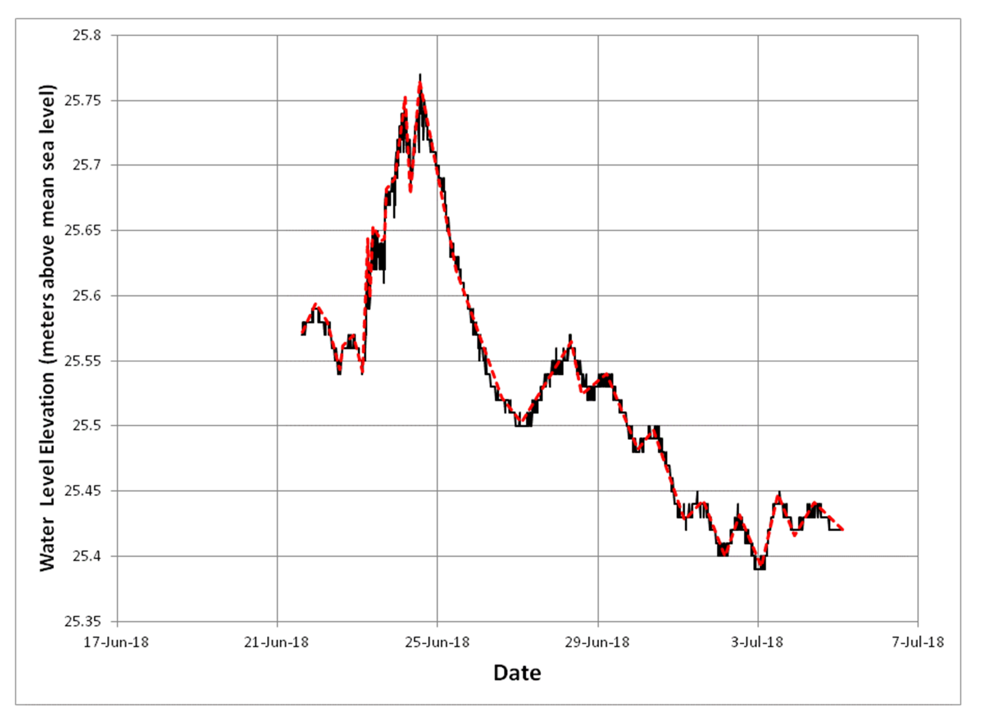
Figure 5.
Complete hydrograph from sensors (black, continuous line) and simplified hydrograph considered (red, dashed line).
Figure 5.
Complete hydrograph from sensors (black, continuous line) and simplified hydrograph considered (red, dashed line).

Figure 6.
Complete channel width and average water depth as functions of gauge height for the Sagavanirktok River west channel near MP405 (DSS1). Bankfull water depth at the main channel is clearly defined in the plot (red oval).
Figure 6.
Complete channel width and average water depth as functions of gauge height for the Sagavanirktok River west channel near MP405 (DSS1). Bankfull water depth at the main channel is clearly defined in the plot (red oval).

Figure 7.
Grain size distributions from samples collected upstream of pits at DSS3 and DSS4.

Figure 8.
Example of sensitivity analysis performed at DSS2.


Table 1.
Date of bathymetric surveys at pits.
| Site Name | 2015 | 2016 | 2017 | 2018 |
|---|---|---|---|---|
| Sagavanirktok River MP405 (DSS1) | September 14 | June 27–28, August 1, September 1 | July 8, August 5, September 6 | July 5, August 9, September 10 |
| Sagavanirktok River downstream Ivishak River (DSS2) | September 10, September 13 | June 30–July 1, August 2, August 31 | July 9, August 6, September 7 (dry pit only) | July 4, August 7, September 13 (dry pit only), October 23 (dry pit only) |
| Sagavanirktok River at Happy Valley (DSS3) | September 18 | July 2, Aug 3, September 3 | July 7, August 4, September 5 | August 11, September 7, October 24 (dry pit only) |
| Sagavanirktok River near MP318 (DSS4) | September 16 | July 3, August 4, Aug 30 | July 6, September 4 | August 12 |
Table 2.
Maximum particle size moved after breakup—Sagavanirktok River at Happy Valley (DSS3).
| Date | Maximum Water Level Elevation (m AMSL) | Average Water Depth in the Main Channel (m) | Slope | (N/m2) | τ *crit | Sediment Diameter (m) |
|---|---|---|---|---|---|---|
| 6/21/2016 | 289.53 | 1.42 | 0.0032 | 44.577 | 0.03 | 0.092 |
| 7/25/2017 | 289.56 | 1.45 | 0.0032 | 45.518 | 0.03 | 0.094 |
| 8/18/2018 | 289.88 | 1.77 | 0.0032 | 55.564 | 0.03 | 0.114 |
Table 3.
Maximum particle size moved after breakup—Sagavanirktok River near MP318 (DSS4).
| Date | Maximum Water Level Elevation (m AMSL) | Average Water Depth in the Main Channel (m) | Slope | (N/m2) | τ *crit | Sediment Diameter (m) |
|---|---|---|---|---|---|---|
| 6/22/2016 | 370.24 | 1.93 | 0.0032 | 60.587 | 0.03 | 0.125 |
| 7/25/2017 | 370.2 | 1.89 | 0.0032 | 59.331 | 0.03 | 0.122 |
| 9/1/2018 | 370.5 | 2.19 | 0.0032 | 68.748 | 0.03 | 0.142 |
Table 4.
Pit volume change between consecutive surveys.
| Period | Volume Change (m3) | |||
|---|---|---|---|---|
| DSS1 | DSS2 | DSS3 | DSS4 | |
| 2015/2016 | 140 | 136 and 126 | 64 and 21 | 35 and 10 |
| 2016/2017 | 62 | 9 | ||
| 2017/2018 | 58 | 84 | 52 | 15 |
| 2018 | 58 | 46 | ||
Table 5.
Alpha values and associated error for each station.
| Station | Alpha | Average Error (%) | |
|---|---|---|---|
| Range | Average | ||
| DSS1 | 0.04 to 0.06 | 0.045 | 5 |
| DSS2 | 0.01 to 0.02 | 0.015 | 37 |
| DSS3 | 0.02 to 0.07 | 0.037 | 31 |
| DSS4 | 0.006 to 0.02 | 0.012 | 25 |
© 2020 by the author. Licensee MDPI, Basel, Switzerland. This article is an open access article distributed under the terms and conditions of the Creative Commons Attribution (CC BY) license (http://creativecommons.org/licenses/by/4.0/).
Share and Cite
MDPI and ACS Style
Toniolo, H. Bed-Sediment Transport Conditions along the Sagavanirktok River in Northern Alaska, USA. Water 2020, 12, 774. https://doi.org/10.3390/w12030774
AMA Style
Toniolo H. Bed-Sediment Transport Conditions along the Sagavanirktok River in Northern Alaska, USA. Water. 2020; 12(3):774. https://doi.org/10.3390/w12030774
Chicago/Turabian StyleToniolo, Horacio. 2020. "Bed-Sediment Transport Conditions along the Sagavanirktok River in Northern Alaska, USA" Water 12, no. 3: 774. https://doi.org/10.3390/w12030774
Note that from the first issue of 2016, this journal uses article numbers instead of page numbers. See further details here.