Addressing the Water–Energy Nexus by Coupling the Hydrological Model with a New Energy LISENGY Model: A Case Study in the Iberian Peninsula

Abstract

As water is required for producing hydropower, and subsequently the water balance is changed for downstream areas, the linking of hydrological and energy models is needed to properly address the interactions among them. In this study, volume–depth-based water storage estimation models were proposed for individual lakes and reservoirs in the Iberian Peninsula using the 30-year Global Water Surface dataset and reservoir morphometry methodology which enables to evaluate reservoirs where data were not available before. The models were subsequently implemented within the new hydropower model called LISENGY that provides the first comprehensive assessment of the temporal and spatial dynamics of water storage, water depth and hydropower production in the Iberian Peninsula. The LISENGY model was coupled with the distributed LISFLOOD hydrological model. The seasonal and interannual changes in energy production were assessed for 168 studied reservoirs with diverse morphometries, which is unique. Conical, concave and convex regression reservoir relationships were distinguished, and optimized turbine discharge and power production were computed. A 10-year water–energy linked system for the 2007–2016 period has been established for the Iberian Peninsula which was not available before. The results showed that it is possible to connect those two models and that the timing and magnitude of simulated storage were well reproduced. The study represents the first step towards integrated pan-European water–energy modeling. Future climate scenarios and energy demands are to be fed into the linked model system to evaluate expected future hydropower generation and possible water scarcity issues.

1. Introduction

Accurate and timely information about reservoir area, water storage and water depth are essential for various purposes such as irrigation and livestock watering, flood protection, recreation, groundwater recharge, fisheries and power production [1,2]. This is particularly important for the Iberian Peninsula where drought mitigation, agricultural irrigation and hydropower production are becoming more vulnerable with changing climate. In addition, hydropower generation as a source of renewable, reliable and affordable energy is considered nowadays as one of the sustainable development goals (UN, Goal-7, https://sustainabledevelopment.un.org/sdg7).

The potential energy from a reservoir is linked to reservoir morphometry, meteorological conditions and hydrology. Variations in any of these fields would alter the storage capacity of a reservoir and energy production potential [3,4]. Many hydrological models have simplistic reservoir routines, but these routines usually are driven by hydrological processes and not by energy production [5].

Over the last 30 years, there has been a proliferation of hydropower models developed by many institutions and researchers around the globe. Some of the models have their own GUI and optimization techniques (i.e., RiverWare [6], ModSim [7], HydSim [8], COLSIM [9]). The others do not have any optimization capabilities (i.e., HEC-Res-Sim [9]) but they contribute to decision-making processes for reservoir operations and planning. Some models focus on water use and its availability within the sustainable management practices (i.e., WATERGAP [10], WEAP [11] and WATERSIM [12]).

One of the recent water–energy models addressing energy and water demands on larger scales is the CLEW model [13], applied at the country level. The authors of this framework used previously developed individual models for water, energy and land-use rather than developing a fully new integrated model from scratch. They coupled them by using exchange modules so that the output of one model was an input to the other two models that were solved sequentially. However, many of these models are constrained to a coarse spatial resolution (>100 km) including regional and national scales and are run on a monthly or even yearly time step which makes it more difficult to address many of the water-related issues.

High spatial (i.e., 1 km/5 km) and temporal (i.e., day) hydropower modeling is therefore needed for assessing the effects of climate variability and human activities on water resources availability and security. Being able to estimate for each reservoir the water storage, depth and hydropower generation in water-scarce regions such as the Iberian Peninsula could contribute to a better understanding of long-term climate change and water availability and thus would provide a first comprehensive map of reservoir energy availability in the Peninsula.

Water storage of natural lakes and reservoirs in the Iberian Peninsula has been rarely studied. In theory, the estimation of water storage requires both bottom topography and water level, where water storage can be derived as a difference between the water depth and the bottom. Determining the reservoir bathymetry of a reservoir is a challenge since it requires expensive equipment and labor and it is time-consuming. Thus, obtaining the bottom topography of dozens of large water bodies in the Iberian Peninsula seemed to be an impossible task. On another side, water levels in the reservoirs are regulated by hydropower operators who produce energy by discharging water through turbines. Level fluctuations in such reservoirs are often not publicly available given the commercial interests of the reservoir operators. Given that, there is a need to develop integrative hydropower models that indirectly estimate water levels and releases, and hence power generation, thus including the economic aspect of reservoir operation strategies. Water is needed to produce energy, and in return, energy is used to clean and transport water. This linkage, known as the water–energy nexus [14] needs to be developed jointly by finding long-term solutions to energy demand due to climate change and anthropogenic influences.

Considering the data unavailability from dam operators, one of the main objectives of this study was, therefore, to derive volume–area–depth water storage estimation models for reservoirs in the Iberian Peninsula using measurements of a dam and reservoir itself. In the last 10 years, many efforts have been made to monitor surface water dynamics over the globe [15,16,17]. Most of these works used LANDSAT images to measure and monitor reservoir areas and derive volume variations. Regardless of the applicability of the methods used in those studies, the crucial question was how to establish the relationship between the storage capacity of the reservoir and surface area and/or reservoir depth when faced with lack of data.

As the storage of the reservoir is often highly correlated with surface area [17,18,19] or depth [20,21,22], empirical volume–area–depth relationships can be estimated by using remotely sensed maximum water areas and reservoir characteristics. These relationships are responsible for flood routing, hydropower generation and reservoir classification [23]. The more complex the morphometry of a reservoir is, the more difficult it is to establish such a relationship [24]. An overview of possible reservoir shapes with respect to their concavity and different cross-sections is presented in [25].

In the present study, we propose a hydropower model, LISENGY, that uses the discharge from the hydrological model LISFLOOD. We present a model that simulates water levels and power production at a daily time step at a fine resolution (5 × 5 km grid). The coupled hydropower model allowed to assess the storage levels and energy production from reservoirs and enhance our scientific understanding about reservoir management operations in the water–energy nexus framework.

Motivated by the need for accurate higher temporal and spatial resolution information about reservoir water storage and power production in our hydrological models, this study thus had the following objectives:

(a)

Derive the empirical models and volume–depth relationships to quantify the reservoir storage using long-term remotely sensed maximum water areas from a 30-year Global Water Surface dataset [26] which enables to evaluate reservoirs where data were not available;

(b)

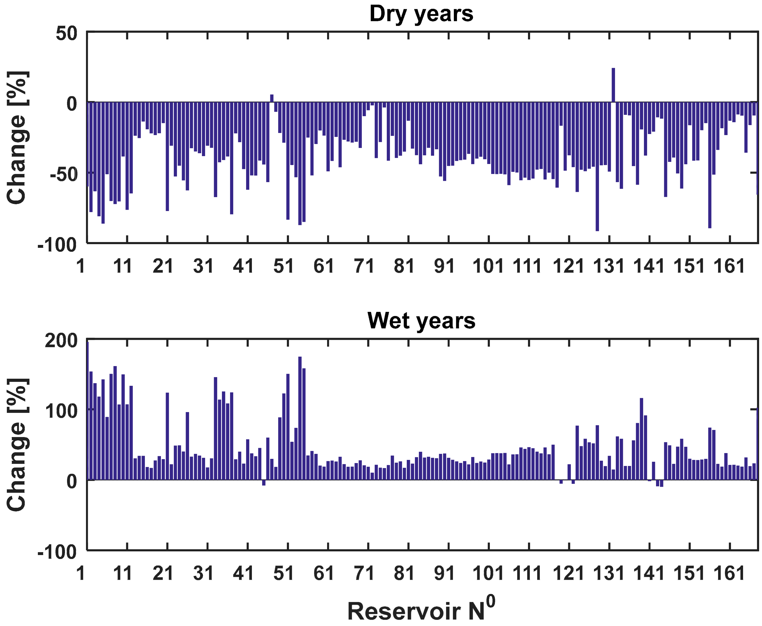
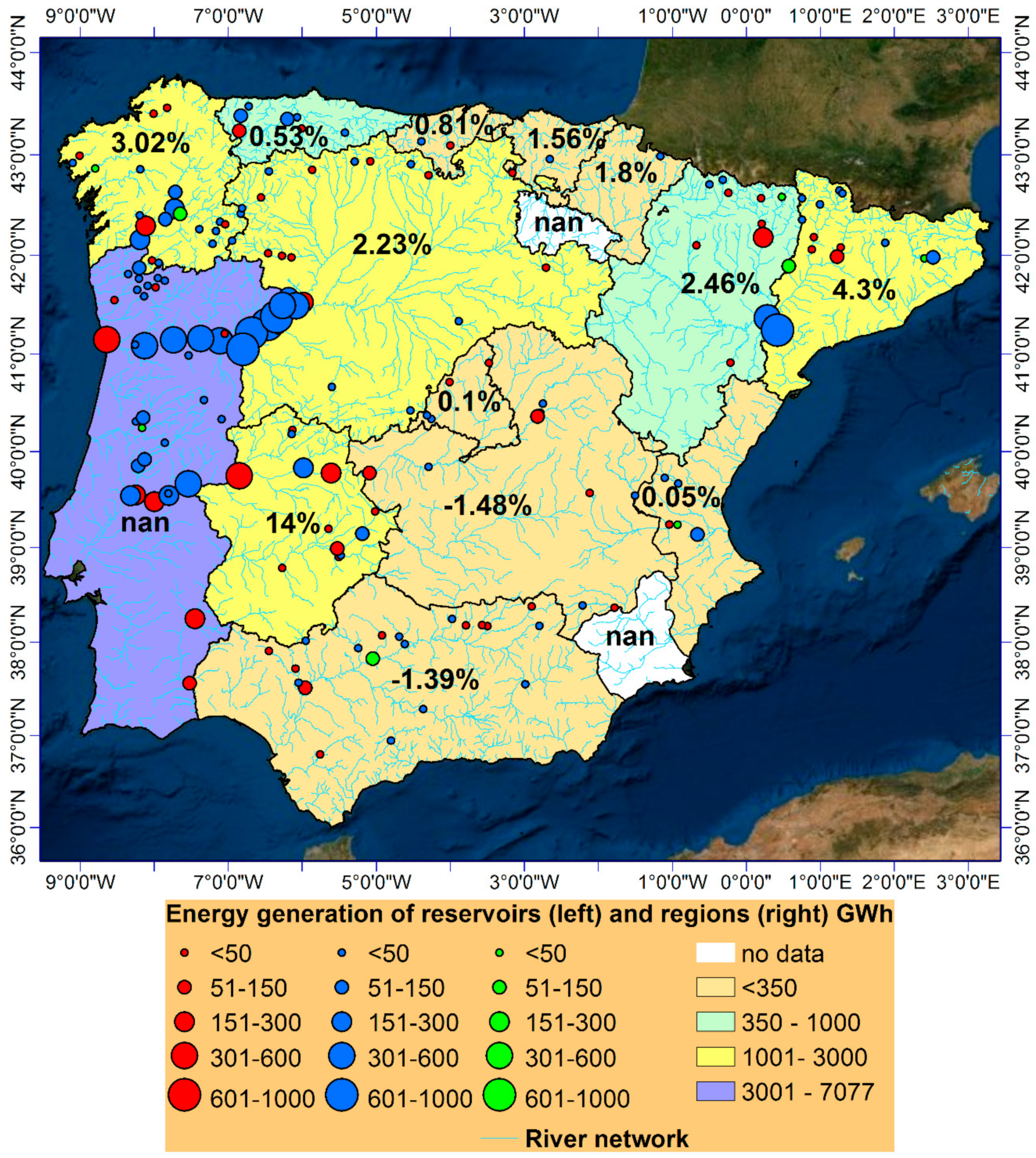
Build a new hydropower model and observe the seasonal and interannual changes of energy production for 168 studied reservoirs in the Iberian Peninsula, which is unique;

(c)

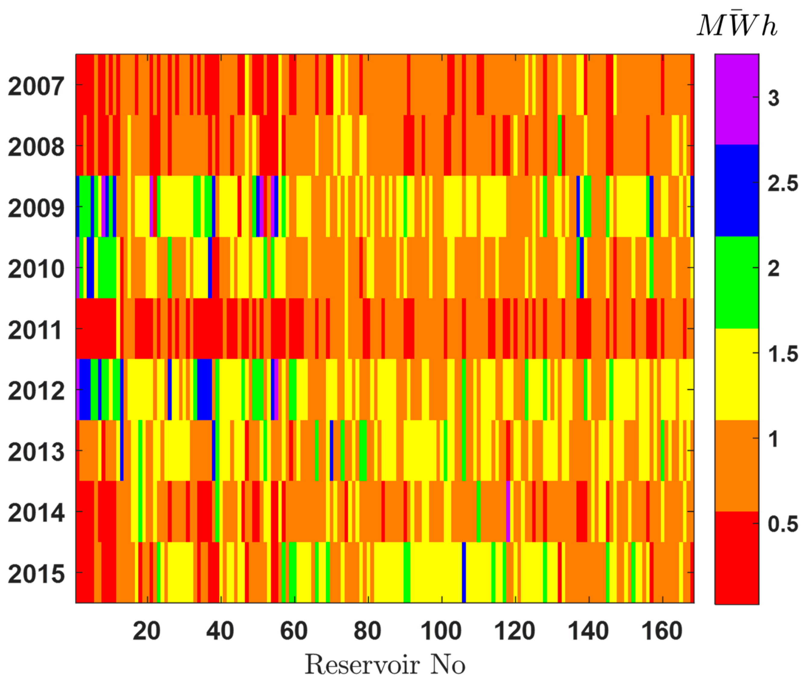
Establish a 10-year water–energy linked system for the 2007–2016 period for the Iberian Peninsula which was not available before and thus evaluate the temporal and spatial dynamics of water storage for each reservoir’s cross-section shape and assess hydropower potential at regional and reservoir level that can serve as an important source of information for future modeling with changing climate.

The paper is organized as follows. Section 2 presents the data used in this study, giving an overview of the reservoirs, inflow and price data. To derive the volume–depth relationships and categorize reservoirs we did morphometric analysis followed by the hydropower model development (Section 3). Section 4 gives a description of the results; finally, the conclusions and recommendations are given in Section 5.

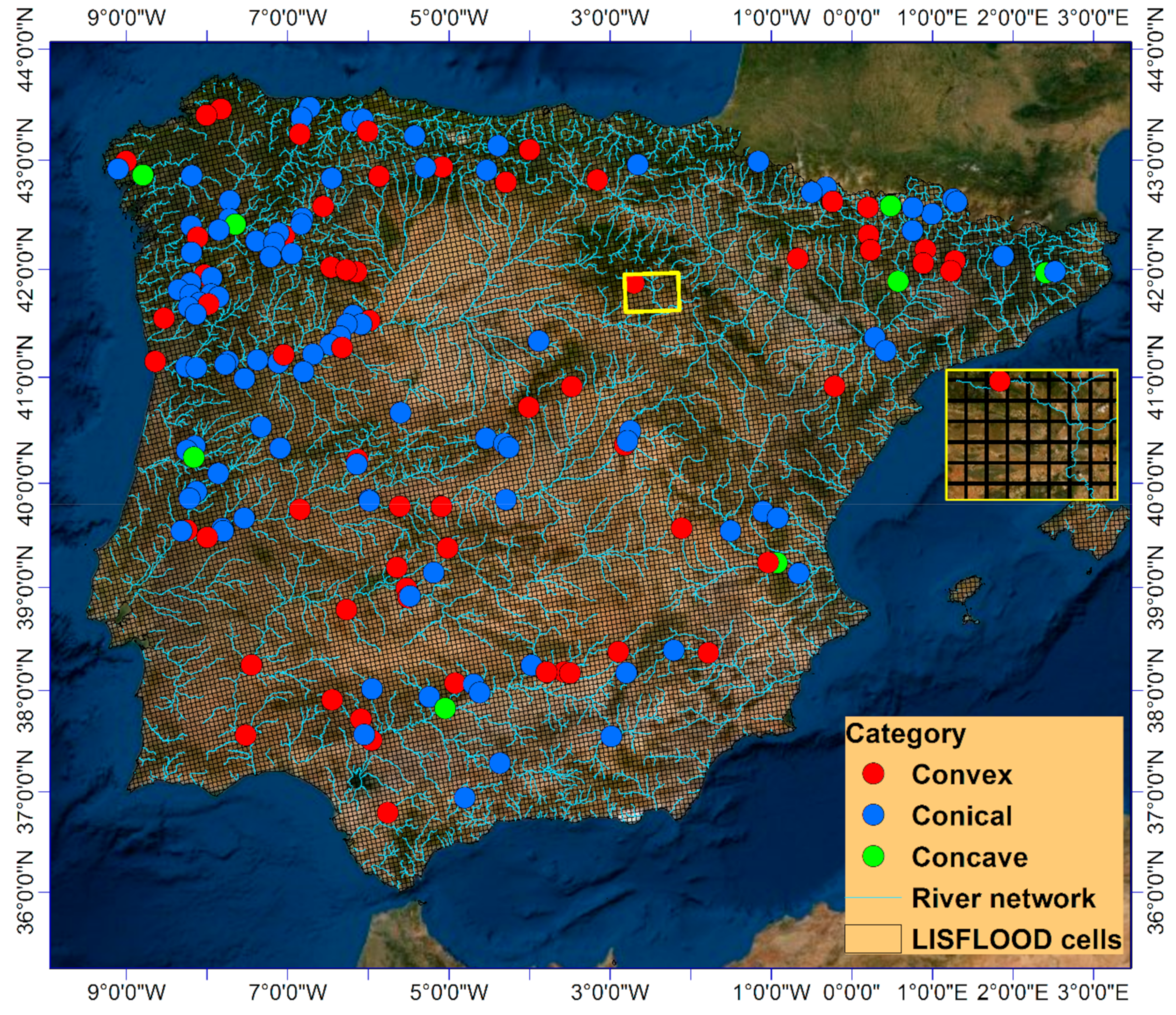
2. Study Area and Data Used

In this section, the study area and the main data are presented. First, we described the study area followed by an overview of the used reservoir data and a brief description of the selection criteria. Then, we presented the reservoir inflow time series and finally the electricity price evolution for the study period.

2.1. Study Area

The study area was the Iberian Peninsula (Figure 1). According to ICOLD (International Commission on Large Dams) (http://www.icold-cigb.net/article/GB/world_register/general_synthesis/number-of-dams-by-countrymembers). Spain has registered 1063 large dams, whereas Portugal has 217 large dams distributed across its territory. Many of its reservoirs have multiple purposes aimed for either domestic water supply, irrigation and agricultural use, electricity production, recreational use, navigational and/or other use. In this study, reservoirs with water use priority for electricity production were considered.

For the Iberian Peninsula, the installed electricity capacity doubled between 1995 and 2015. In the last 10 years, 537 installed hydropower plants generated an average of 42,000 GWh of electricity each year (red.es; ren.pt). Both Portugal and Spain are signatories of the Paris agreement and they are working towards a sustainable energy supply to achieve the reduction of 40% of carbon emission by 2030. According to the 2017 Spanish Electricity System report (https://www.ree.es/sites/default/files/11.../2017/spanish-electricity-system-2017.pdf) 46.3% of the energy-generating facilities in Spain already are renewable. Portugal, with its 67% of the installed renewable share, confirms the country’s firm and renewable deployment strategy. Figure 2 shows the variable year-to-year hydropower generation in Spain. We also observed the increasing presence of renewables in the last 10 years along with the fossil fuels reduction of about 25% in the whole Iberian Peninsula.

This case study was a part of the WATERFLEX project [27], which aimed at assessing the potential of hydropower to make the European power system more flexible and less carbon-dependent.

2.2. Data Used

2.2.1. Reservoir Data and Characteristics

Reservoir data was obtained from the Global Reservoir and Dam Database (GRanD) (http://www.gwsp.org/products/grand-database.html) and www.cedex.es. GRanD includes reservoirs with a storage capacity of more than 0.1 Hm³. Among them, 168 reservoirs in the Iberian Peninsula were selected in this study with surface areas of >0.1 km² and capacities of >0.35 Hm³ (Figure 1). For a reservoir to be selected, the following information was needed: the maximum water depth (Hmax (m)) defined as a difference between the dam crest and the lowest point in the reservoir, the maximum surface area of the reservoir (Amax (m²)), the maximum volume of the reservoir (Vmax (m³)) and the maximum power capacity (Gmax (MWh)). Hmax, Vmax and Gmax were obtained from the Spanish (www.cedex.es) and Portuguese authorities (https://www.apambiente.pt/) and JRC Petten database [28].

To estimate the maximum reservoir surface, we used the recently derived JRC Global Surface Water (GSW) dataset [26]. The GSW dataset is a highly accurate surface water dataset on 30 m resolution which includes the whole L1T Landsat 5, 7 and 8 archive, allowing detailed global area calculations over a very long period. It has many derived layers. We used the maximum water extent, which provides information on all water bodies over the 32 years. These datasets are available in tiles of 10° × 10°.

2.2.2. Reservoir Inflow Data

The inflow data for reservoirs were modeled with the LISFLOOD 2.0 hydrological model [29]. LISFLOOD is a GIS-based spatially-distributed hydrological rainfall-runoff model [30,31]. Driven by meteorological data, the LISFLOOD model calculates a complete water balance at a daily time step simulating the most important physical processes (e.g., surface runoff, infiltration, evapotranspiration) for every grid-cell (5 × 5 km). The produced runoff is routed through the digital river network. More details on the model setup can be found in [31]. LISFLOOD was successfully applied at European, African and global scales for applications for flood forecasting [32,33] as well for policy impact studies dealing with climate change impact assessments [34,35].

For this work, LISFLOOD was run on the Iberian Peninsula domain at 5-km resolution and daily time step from 1 October 2007 until 30 September 2016. Discharge upstream of the reservoir was used as a proxy for the reservoir inflow.

Simulated inflows of the 168 reservoirs are given in Figure 3. We noted the high discharge variability between the reservoirs. Maximum inflows ranged between 2 and 4154 m³/s, while the mean flows ranged between 0.4 and 600 m³/s. The quality of the simulated inflow data was a key variable in this hydropower modeling study. High average simulated inflows resulted in high outflows and consequently in a high-energy generation to achieve dam target operations in the LISENGY model. In

Table 1. Average monthly inflows (m³/s) for the ensemble of reservoirs for 2007–2016 study period.

Months	January	February	March	April	May	June	July	August	September	October	November	December
Inflows	98.6	101.3	99.8	99.9	70.3	43.3	24.9	19.4	18.2	26.2	46.5	58.3

, the average monthly flows of all hydrological years and all reservoirs are shown. We observed the highest inflows into the reservoirs during January–April. Dam operators have to optimize reservoir outflows to satisfy peak energy demands in the Iberian Peninsula occurring in November–March and June–August (source: www.ree.es).

2.2.3. Price Data

The market-based system is presented in the Iberian Peninsula where the majority of the activities are regulated by private owners. The main market players are the market operator OMIE (http://www.omie.es/en/home/information-company), which comprises both Spain and Portugal, and the system operators of Spain, REE (Red Eléctrica de España), and Portugal, REN (Redes Energéticas Nacionais).

Regarding the electricity prices, historic hourly data of the day-ahead electricity markets both of the Spanish zone and the Portuguese zone were obtained from OMIE. We chose the hydrological years 2007–2016 as a study period since the Portuguese Market started in July 2007, operated by OMIE after the signature of the International Treaty by the Governments of Spain and Portugal. It should be mentioned that there are two bidding zones, but both countries are quite well interconnected, so the price difference among countries was small, with 94.4% of hours having a price difference under 1 €/MWh throughout the examined period (Figure 4).

3. Modeling Framework

In this chapter, we first presented the conceptual framework for hydropower modeling. Then, a morphometric analysis for reservoir categorization was described. We investigated here whether simple reservoir morphometric characteristics can be used to approximate volume–depth reservoir relationships among the range of different environmental and geographical settings. Then, the proposed LISENGY hydropower model and its optimization were described. Finally, we provided a brief description of model validation techniques.

3.1. Overview

The method used to build the water–energy nexus framework was twofold. Figure 5 shows a schematic diagram of the study framework used in this paper. The modeling framework consisted of combining the two following modeling tools: (1) the daily LISFLOOD hydrological model and (2) the proposed LISENGY model based on the volume–depth relationship. The interaction among models was organized as follows:

• LISFLOOD provided the inflows into the selected reservoirs. Those inflows were fed directly to the daily hydropower LISENGY model that simulated water level and discharge for hydropower production.
• LISENGY established the operational power system rules of hydropower plants for a determined period (one hydrological year) and optimized releases to maximize profit subject to equality, inequality and operational constraints derived from the power system rules (see optimization in Section 3.4).
• Coupling between LISFLOOD and LISENGY was done by external communication (data coupling) where outputs from LISFLOOD at the matching cells (i.e., upstream from the reservoir) became inputs to LISENGY without defining any internal boundary condition between them.

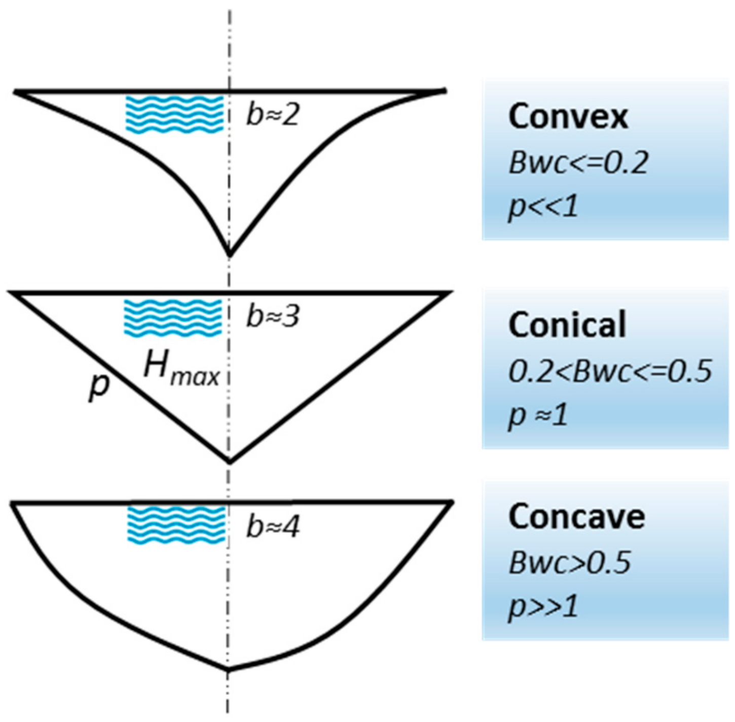
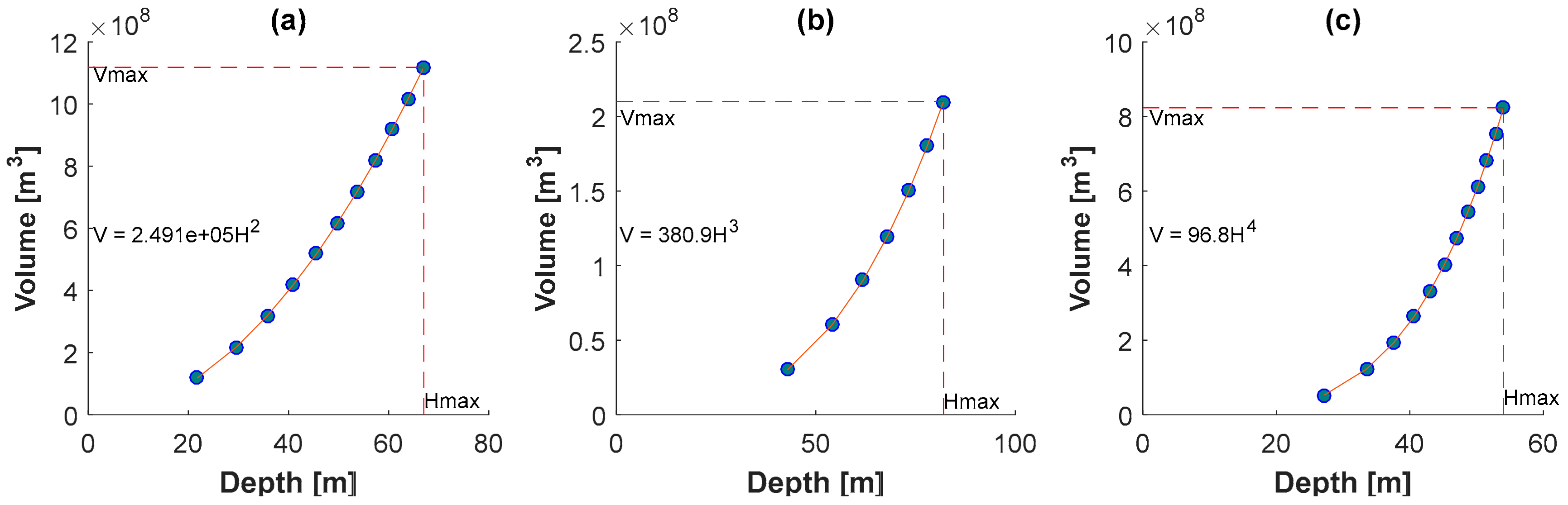
3.2. Volume–Depth Morphometry Approximation

The volume–depth approximation represented the first step in developing the LISENGY hydropower model. Power plants are constructed in different natural and geomorphological conditions with different geometries. Correlation between volume, area and depth of the reservoir is well known and the general assumption here is that the reservoir area and depth are monotonically increasing functions of volume [36]. The rate of such change is dependent on the slope. When slope changes, hydropower production also changes. Thus, the reservoir volume can be defined as a function of their surface area or as a function of depth. In this study, we used the volume–depth relationship that can be expressed as a power function of the form:

$$V=\alpha \times H^b$$

(1)

where V is the estimated storage and H is the water depth of the reservoir. Both $\alpha$ and b are constants, where $\alpha$ represents the openness of the reservoir (the flatter the valley, the larger is $\alpha$) and b determines the reservoir hillside slope concavity [22].

Many reservoirs are often either shallow with large surface areas or deep with small surface areas. Reservoirs tend to be more concave when b increases and become more convex when b decreases. The middle average value between convex and concave reservoir shapes in the volume–depth relationship is equal to 3, and it corresponds to the reservoir cut in half like a pyramid and rotated 90 degrees around the x-axis (Figure 6). The average values of parameter b are derived from [25] for each reservoir category.

Reservoir morphometry can be assessed by computing many different variables [23]. Among them, in our study, we used the bathymetric capacity Bwc and the morphometry coefficient p.

The bathymetric capacity represents a reservoir capacity to store water, and it is defined as:

$$Bwc=\frac{V_{max}}{H_{max}\times A_{max}}$$

(2)

where V_max is the maximum volume of the reservoir (m³), H_max is the maximum depth (m) and A_max is the maximum area (m²). Bwc indicates how strong the linear relationship between reservoir storage and dam height is. Bwc of 1 could be taken as a perfectly rectangular-shaped reservoir. These kinds of reservoirs are however usually artificially made and used in urban areas. Therefore, they were not considered in this study, and thus accordingly, reservoirs were classified into three broad shape categories: convex, conical and concave (Figure 6).

The dimensionless morphometry coefficient p represents the shape of the bathymetric curve [37]. It is defined as:

$$p=\frac{2}{\left(\frac{1}{Bwc}-1\right)}$$

(3)

The greater the p, the greater the concavity is; the smaller the p, the greater the convexity is [37].

In order to derive the V-H relationships, we introduced the following four steps:

Step 1: This step consisted of identifying the maximum water extents of all water bodies in the Iberian Peninsula using the Global Surface Water website (https://global-surface-water.appspot.com/download). Reservoirs were filtered from the other types of permanent water bodies (e.g., rivers, depressions) by selecting those that have areas larger than 0.1 km² and that match the location of the 168 reservoirs identified in Section 2.2.

Step 2: The maximum depth of a reservoir and the maximum area were associated with the maximum storage capacity. Maximum depth–area–storage reservoir triplets among the range of different environmental and geographical settings were then used to compute Bwc and the p parameter.

Step 3: The reservoirs were classified into three types thanks to the reservoir bathymetric capacity to store water, Bwc (calculated in Step 2), and the b parameter was set accordingly (see Figure 6).

Step 4: Parameter $\alpha$ for each reservoir was computed using Vmax and Hmax in the inverted form of Equation (1) from which the new depth-based storage reservoir models were developed and implemented in the LISENGY hydropower model. In this study, we assumed that the reservoirs do not change their shape over the study period.

3.3. LISENGY Hydropower Model Development

The proposed LIESNGY hydropower model is described next. The hydropower generation Gt, was calculated as:

$$G_t=\rho g{H}_t{Q}_{tur,t}\mu$$

(4)

where Gt is the hydropower generation (MWh) in day t, $\rho$ is the water density (1000 kg/m³), Ht is the hydraulic head (m) in day t, g is the gravity (9.81 m/s²), Q_tur,t is the discharge through turbine (m³/s) in day t and $\mu$ is the overall hydropower efficiency taken as 0.9 (https://www.usbr.gov/power/edu/pamphlet.pdf) by ignoring the hydraulic loss variation.

Long-term simulations of nine years were employed as a study period. The objective of the LISENGY model was to find discharges that optimize an objective function subject to the equality and inequality constraints (see Section 3.4). It should be mentioned that many costs directly linked to hydropower production were considered to be independent of actual operations (i.e., labor costs). Therefore, in this study, the cost element has been neglected.

Numerous hydrological and operational assumptions about reservoir behavior were established beforehand. Evaporation and infiltration were neglected. The main function of the reservoir was considered to be hydropower production and other types of abstractions (e.g., for industrial, residential and irrigation purposes) were not taken into account. The variation in the storage was the result of the interdependence between the inflow from the upstream catchment area that feeds the reservoir and the reservoir discharge which meets dams’ requirements. Inflow to the reservoir was mainly driven by the precipitation over the catchment area and the start of the operation year for each reservoir was set to October (start of the hydrological year). These model limitations are discussed in Section 4.4.

The maximum hydropower generation was determined for each reservoir based on the current hydroelectric facilities, installed hydropower capacity, storage capacity and dam height. Dam height was considered as the maximum hydraulic head in this study.

In our study, the storage was calculated for each reservoir and each day. The daily storage of the reservoir was computed using the difference of total inflows and total outflows according to Equation (5). The storage balance equation is given as:

$$V_t=V_{t-1}+I_t-{\left(Q_{tur}+Q_{spill}\right)}_t$$

(5)

where V_t is the storage at time t, V_t−1 is the storage at previous time step, I_t is the total inflow into the reservoir at time t and total outflow is equal to the sum of outflows Q_tur(t) and Q_spill(t), which represent the turbine flow and spill flow at time t, respectively.

3.4. Model Optimization

The optimization problem aims at maximizing the total hydropower revenue, which was computed as the sum of daily products of the power generated by a dam and the electricity price:

$$MaxF={\displaystyle \sum }_{t=1}^n{P}_t\times G_t$$

(6)

where MaxF is the revenue of reservoir, n is the number of days, t is the interval time (day) and Pt is the average electricity price on day t (EUR/MWh).

Profit maximization means that the hydropower plant starts discharging water through the turbines when the price is high and when the water level is as high as possible to maximize the revenue of a certain discharge. Equation (6) reflects the economic value of the discharged water for hydropower production that is to be maximized in the given study period.

The optimization is subject to numerous constraints. Equations (7) and (8) show the minimum and maximum bounds on the outflow and storage, respectively.

The water discharge for hydropower production was bound by turbine capacity such that:

$$Q_{tur}^{t,min}\le Q_{tur}\le Q_{tur}^{t,max}\left(H_t\right)$$

(7)

where $Q_{tur}^{t,min}$ represents the minimum discharge at time t and $Q_{tur}^{t,max}$ represents the maximum discharge at time t. The maximum probable discharge through turbines was calculated by considering the maximum water head and the maximum power generation for each dam.

The minimum project flow is a flow that has to be assured downstream of the power plant. This constraint was defined using the minimum flow information (www.cedex.es; https://www.apambiente.pt/) and it is expressed as:

$$Q_{spill\left(t\right)}+Q_{tur\left(t\right)}\ge flo{w}^{t,min}$$

(8)

where $flo{w}^{t,min}$ represents the minimum water flow restriction at time t.

Water storage was constrained by the upper and lower storage level and can be defined as:

$$V^{t,min}\le V_t\le V^{t,max}$$

(9)

where $V^{t,max}$ is the maximum reservoir storage at time t and $V^{t,min}$ is the minimum reservoir storage at time t.

The dam height sets the maximum reservoir storage while the minimum storage is defined as the minimum amount of water that must remain in a reservoir and avoids the dam break. We should mention that the majority of reservoirs were assumed to start with the maximum storage at maximum water levels. However, some reservoirs were simulated with the observed initial levels (source: www.cedex.es) if available.

We used a scalarizing function approach implemented with MATLAB’s fmincon programming solver to optimize Q_tur on each day. Fmincon is a gradient-based method aimed to solve the nonlinear multivariable problems and constraints that are continuous and have continuous first derivatives. The interior-point algorithm was used that is capable of dealing with large and sparse problems. The algorithm iterated until the local minimum was found and the existing constraint conditions of every reservoir were satisfied. We ran a maximum of 5000 iterations for each reservoir independently from the others in the region to find optimized discharge. To deal with the time-consuming calculations, the number of iterations and the number of reservoirs, parallel computing was introduced.

3.5. Model Validation Techniques

For each reservoir category, a comparison with the observed reservoir storage was done to ensure that storage follows the volume–depth curve of each reservoir. To assess model efficiency, we used the coefficient of determination (R²) to quantify the linear correlation between observed and simulated storage using daily storage values. R² ranges from 0 to 1, where higher values indicate smaller error variance [38].

Percent bias (PBIAS) was also calculated as a main part of the model evaluation statistics for characterizing the storage variations. It measures the total volume difference between two-time series, as Equation (10) indicates:

$$PBIAS={\displaystyle \sum }_{i=1}^n\frac{\left(S_i^{obs}-S_i^{sim}\right)\times 100}{{{\displaystyle \sum }}_{i=1}^n{S}_i^{obs}}$$

(10)

where $S_i^{obs}$ is the i-th observation of storage data, $S_i^{sim}$ is the simulated storage value for the i-th time step, n represents the number of observations and 100 converts the result to percent. The optimal value of PBIAS is 0, where positive values indicate model overestimation and negative values indicate model underestimation [39].

4. Results and Discussion

The results section is divided into four parts. In the first part, results concerning the reservoir morphometry and volume–depth relationship of all reservoirs are given (Section 4.1). Then, we present the results of the LISENGY model for three reservoirs with different morphometries (Section 4.2). In Section 4.3, the results regarding the power generation for 168 reservoirs are shown. Finally, in Section 4.4, we discuss the model limitations and choices made in this study.

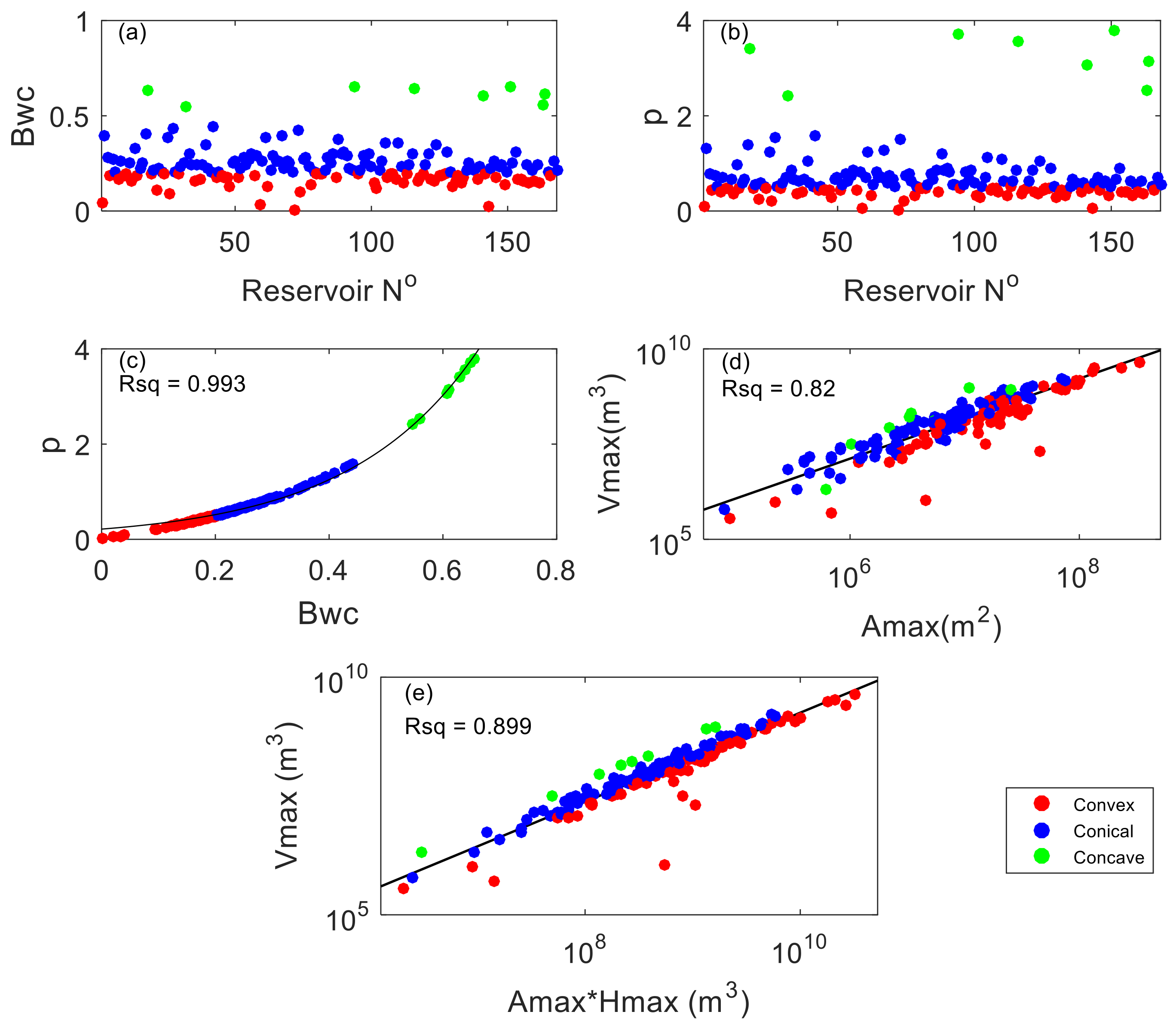
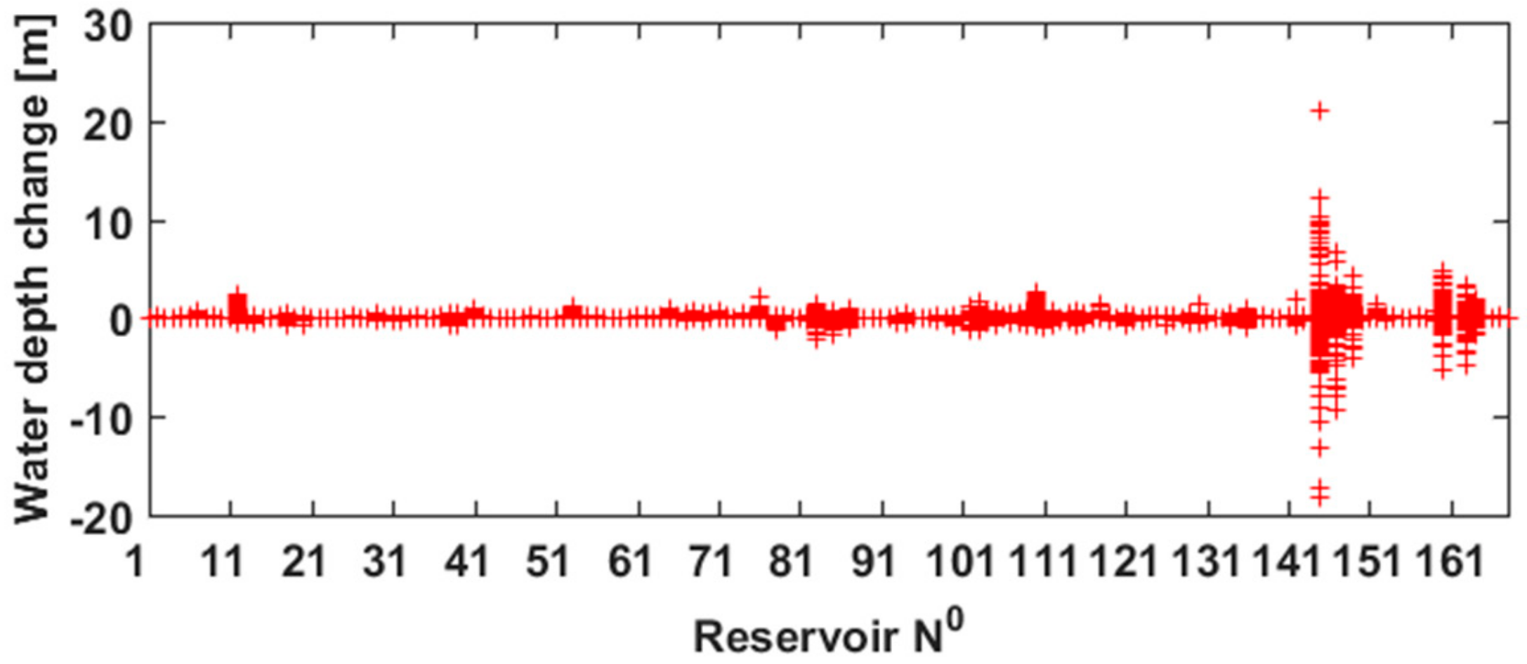
4.1. Reservoir Morphometry

Joint reservoir morphometric characteristics are given in Figure 7. The 168 studied reservoirs were classified into convex, conical and concave morphometry forms (Figure 7a,b) and depth-based storage models were developed. The categorization of reservoirs was done based on Bwc (see Equation (2)). Around 90% of the reservoirs tend to have conical and convex forms. Only eight of them were categorized as concave-shaped reservoirs. The summary of the categorization is shown in

Table 2. Reservoir categorization and their average morphometric characteristics.

Category	Dam Height (m)	Volume (m3)	Area (m2)	Power Capacity (MW)	Q Max (m3/s)	Bwc (-)	p (-)	α (-)
convex	75.21	4.80 × 108	3.46 × 107	121.84	23.75	0.16	0.39	69,136.27
conical	75.24	2.15 × 108	9.97 × 106	131.93	51.02	0.27	0.75	514.51
concave	69.75	2.97 × 108	6.50 × 106	288.73	32.00	0.61	3.20	421.74

. Each variable presents the average of all reservoirs within the category.

Maximum dam heights of all reservoirs ranged from 5 to 225 m with a median of 73 m, which reflects the high hydropower potential of those reservoirs. A gradual increase in the Bwc and the p parameter as the reservoir becomes more concave can also be seen from Table 2. At the same time, α becomes smaller when the surface area is reduced. We can also observe that α for convex-shaped reservoirs is much larger compared to conical and concave-shaped reservoirs. This indicates that convex-shaped reservoirs are located in large, flat valleys with large storage capacities. The higher Bwc is, the greater the expected power generation is.

In Figure 7b, p coefficient ranges between 0.004 and 3.8 (median of 0.56). Over 80% of the studied reservoirs had a p coefficient of less than 1 and thus were categorized as a convex or conical reservoir. Additionally, a strong exponential relationship was found between parameter p and Bwc (Figure 7c). Furthermore, to check whether data fit a power-law relationship in the studied reservoirs, log–log plots were done (Figure 7d,e). In these two figures, the reservoir volume showed strong power correlations to Hmax and Amax with Rsq > 0.82.

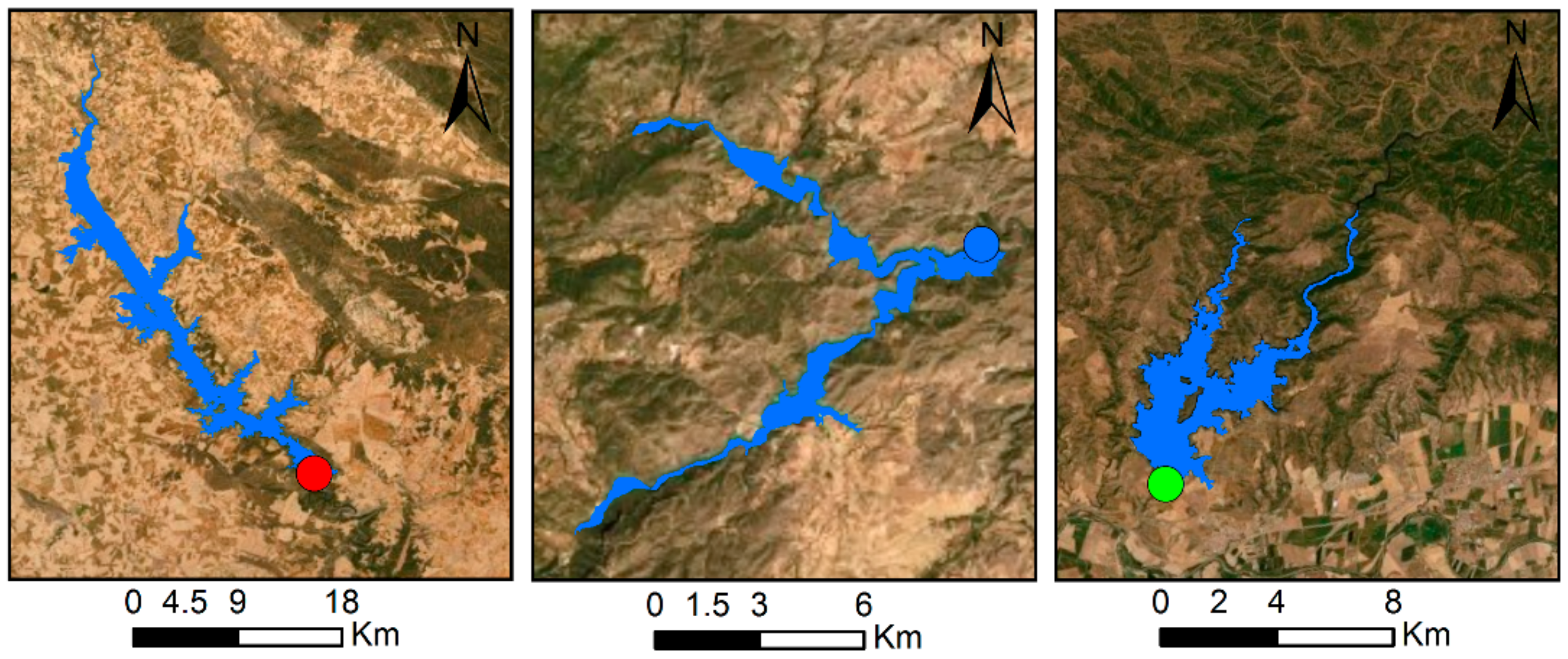
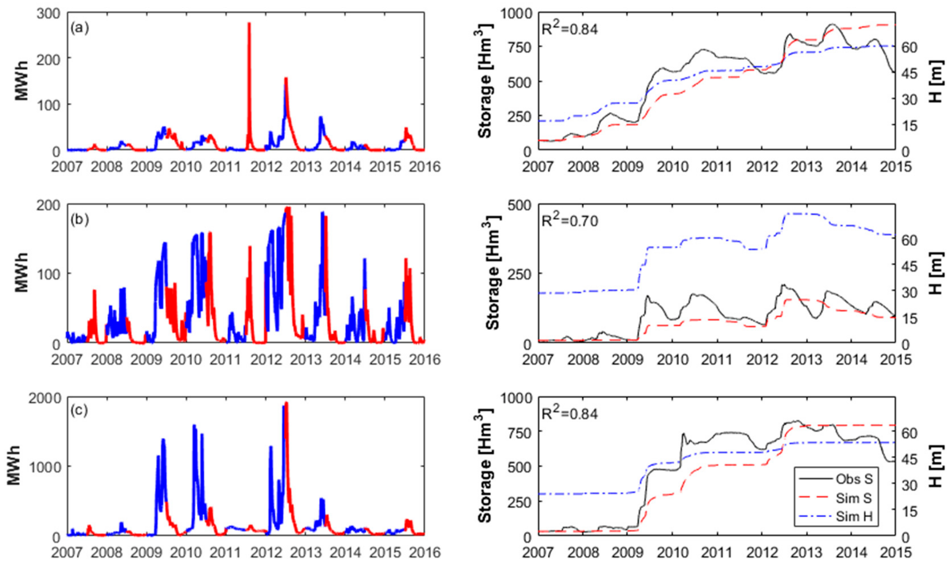
4.2. Study Sites for Water Storage Validation

Validation is an essential step in assessing model robustness, and, therefore, LISENGY was validated against observations. Here, three reservoirs with different shapes were used for the validation. The sites were selected based on data availability for a range set of conditions: river basin, catchment area, power and storage capacity, geographic and morphometric characteristics. Figure 8 shows Alarcon, Fuensanta and La Brena reservoir sites. Their dam characteristics are shown in

Table 3. Alarcon, Fuensanta and La Brena reservoir characteristics (source: MAPAMA).

Reservoir	Alarcon	Fuensanta	La Brena
Latitude	39.57° N	38.39° N	37.83° N
Longitude	2.11° W	2.21° W	5.04° W
River	Jucar	Segura	Guadiato
Catchment (km2)	2937	1208	1494
Dam height (m)	67	82	54
Volume (3	1118	210	823
Area (m2)	97,352,707	8,309,236	25,131,657
Capacity (MW)	56	9	83
Altitude (m)	806	602	121

.

The selected sites for this validation study are briefly described below:

Alarcon reservoir at River Jucar. This reservoir was formed by the gravity dam in the upper course of the Jucar River. It is located in the province of Cuenca, in the autonomous community of Castilla–La Mancha. It has a water capacity of 1118 cubic hectometers with a dam height of 67 m and a catchment area of about 2937 km². Next to the dam, a hydroelectric power plant is located with an installed capacity of 56 MW. The reservoir is part of the Tagus–Segura Water Transfer system, one of the largest hydraulic works ever done in Spain.

Fuensanta reservoir at River Segura. Fuensanta dam is a gravity dam located on the Segura River with a 1208 km² catchment area. The main uses of the reservoir are flow regulation to meet the demands of irrigation, supply and hydropower production in the municipality of Yeste, province of Albacete. The installed capacity is 9 MW and the storage capacity is 210 cubic hectometers with a dam height of 82 m.

La Brena reservoir at River Guadiato. It is one of the largest reservoirs in the province of Cordoba, in the autonomous community of Andalucia, southern Spain. The storage capacity is 823 cubic hectometers. The benefit of this large volume is that the surplus flow, through a pumping station, can be stored in the reservoir aiming to keep water available for the summer, when it is necessary for the irrigation of the basin and therefore generating the highest amount of hydroelectric energy. The latter is possible thanks to the gravity dam called La Brena II, located near the municipality of Almodovar del Rio. The height of the dam is 54 m, and it has an installed capacity of 83 MW. The reservoir’s drainage area is 1494 km², which is a part of the Guadalquivir basin.

The volume–depth relationships of all three reservoirs were well represented by power functions (see Section 3.1; Figure 9). One can visualize a range of values of parameter b (2–4). As b takes a larger value, the reservoir becomes more concave. We can also note that Alarcon (Figure 9a), as a convex-shaped reservoir, had the highest α coefficient, reflecting the large openness of the reservoir and valley. On the other side, La Brena reservoir had the smallest α coefficient among the three, which emphasizes its concavity.

Depth-based storage reservoir relationships were implemented into LISENGY. Continuous simulations were performed for the whole 2007–2016 period. The daily storage of the reservoir was calculated using the daily inflow and outflow, which was compared with the observed reservoir storage for the period 2007–2015 (observed data after 2015 were not available). Figure 10 shows the daily energy generation in the winter (October–March, in blue) and the summer period (April–September, in red) and comparison between simulated and observed storage with level fluctuations for the three reservoirs.

We note in Figure 10 that all three reservoirs show satisfactory performance for the whole simulation period with R² varying between 0.70 and 0.84. Additionally, in

Table 4. Model performance (PBIAS (%)) of simulated versus observed storage for period 2007–2015 for three reservoirs.

Hydrological Year	Alarcon	Fuensanta	La Brena
2007	6.46	15.39	23.36
2008	23.49	52.15	30.24
2009	30.68	52.47	41.66
2010	28.81	45.13	32.51
2011	15.28	21.29	28.40
2012	−0.71	20.05	10.78
2013	−2.77	6.79	-5.70
2014	−24.36	18.55	−21.58
2015	6.46	15.39	23.36

, model performance summary (PBIAS) for each year and the given reservoir is shown. For all three reservoirs, we observed a good PBIAS performance for year 2007 and the period 2012–2015 where PBIAS was up to ±25%.

Table 4 also points out that the year-to-year variations in PBIAS were sometimes large with some very good results in some years and poor results in other years. This could be a major challenge if the model would be used for real-time operations, which are done at a subdaily scale. Instead, the purpose of the model was to perform long-term assessments. In spite of the volume differences, the simulated storage is correlated well with the observed storage throughout the examined period.

From Figure 10 (left), we can observe that the highest amount of energy was mainly produced in winter times (October–March) and the hydrological years of 2009, 2010 and 2012. However, we observe from Figure 10a (left) and Figure 10b (left) that, in 2011, the highest energy production was in summer periods. Year 2011 can be in general considered as a dry year (see Figure 12). Amidst higher temperatures, higher energy production in summer could be explained due to the higher electricity demand for air-conditioning and higher average daily electricity consumption peaks. Among three dams, La Brena reservoir showed the highest potential with an average production over those three years of 117,422 MWh, whereas Alarcon and Fuensanta produced 7147 MWh and 23,627 MWh, respectively. The highest production of La Brena power plant can be related to the maximum installed capacity of 83 MW. Overall, minimum energy production was observed in the hydrological year 2007 where the whole Iberian Peninsula faced the worst drought in nearly half a century (https://core.ac.uk/download/pdf/6294119.pdf). We also observe the trends of increasing and decreasing of reservoir depth that follow storage trajectories. These dotted blue curves can be seen as rule curves, and they determine target water levels as a function of the time of the year for the reservoir to meet its operational objective.

Many intervariable dependencies coexist together in the LISENGY model in order to maintain ecosystem functioning and provide water and energy supply to people. Deeper reservoirs do not necessarily mean more energy production as energy production also depends on inflow data, reservoir initial storage and restrictions on the rate of dam outflows. These ramp-down and ramp-up rates were defined through model constraints (see Section 3.4 for more details). As aforementioned, the outflows and thus energy production also depend on the price market. Dam reservoir operators are guided by profit maximization, generating and selling more energy if possible in moments when the price is high. For instance, in Figure 2, we can observe three overall market price peaks in 2007, 2008 and 2013. The highest energy market price was established in 2013, 93.11 EUR/MWh. Accordingly, the highest energy production was simulated in the year 2012/2013 (Figure 10). In contrast, even though we observed on average a high energy price in 2007 and 2008, simulated hydropower production was limited by the small storage capacity, inflows and precipitation. In the years of 2007, 2008 and 2011, the Iberian Peninsula was hit by the most severe droughts ever recorded [40,41]. These drought events had important socioeconomic impacts resulting in the decrease of agricultural and hydroelectric power production [42]. In these years, the dry winters and reservoir filling in springtime probably led to higher energy production in summer as can be observed in Figure 10 (left and in red). Besides, in 2007, in Catalonia, a total loss of about 1.7 million EUR has been determined [41] which was equal to almost 1% of the GDP in Catalonia. Many recent works highlight an increase in the frequency of drought events in the Mediterranean [43,44] and particularly over the Iberian Peninsula [45]. The more alarming situation with more frequent dry periods in future climate is to be expected [46].

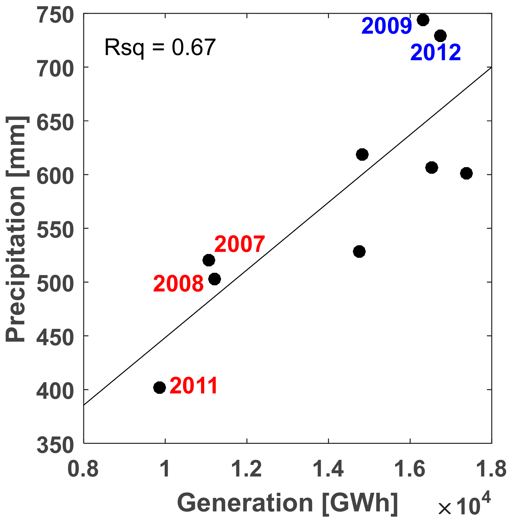
4.3. Power Generation over the Iberian Peninsula

The proposed LISENGY model was applied to 168 selected reservoirs in the Iberian Peninsula. One of the most important outputs of the LISENGY model was the reservoir level. Figure 11 shows the water level change between two consecutive days during the whole study period. Sign change means either a relative increase or decrease of daily water depth. Note that the amplitude of water depth fluctuations varies across the reservoirs, mainly influenced by hydropower production. Besides this main function of a reservoir of emptying and filling for energy production, water depth might also increase or decrease due to inundation and extreme events or shoreline erosion. High amplitude will result in higher energy generation. These water depth fluctuations represent a probable operating curve of power plants. As mentioned in the introduction, it is hard to obtain water depth fluctuations, and hence their model estimation represents one of the most important outcomes of this work.

To assess if energy production is influenced by the interannual precipitation variability, a correlation between these two variables is derived in Figure 12. A variable year-to-year energy generation is plotted against the average annual precipitation. We found that precipitation patterns in the Iberian Peninsula affect dams’ operations showed by a coefficient of determination of 0.67. Overall, we determined that reservoirs facing a dry and warm climate with precipitation less than 520 mm/year showed a decline of hydropower generation from 2007 to 2016. These dry years were marked as critical periods and are highlighted in red in Figure 12. On the contrary, reservoirs in wet conditions with precipitation more than 720 mm/year showed an important increase in hydropower generation. The average energy generation was about 14,300 GWh, reaching its maximum in the years 2009, 2012, 2013 and 2015. We also computed the coefficient of determination between inflow that represents the upstream catchment’s water balance and simulated hydropower production. Over 80% of the studied reservoirs showed a good correlation, with R² > 0.6.

We also analyzed the changes in the inflow discharge by calculating composite anomalies of discharge (%) for the top three dry years and top two wet years from the 2007–2016 period. Figure 13 shows the discharge during the dry years (2007, 2008 and 2011) with a significant deficit (more than 41% on average), suggesting that droughts have negative effects on discharge and related hydropower production. Similarly, during the top two wet years (2009 and 2012), the discharge of all reservoirs was higher than 48% on average of its long-term mean. Thus, our results reflect the influence of climate variability and extremes on discharge and hydropower production in current conditions. We also observed that few reservoirs in both cases show opposite sign changes. This could be due to the uncertainty in the meteorological forcing fed into the LISFLOOD model and most likely due to the strong spatial variability in precipitation.

Figure 14 shows the average 2007–2016 simulated hydropower energy generation. Larger circles correspond to higher hydropower generation. We found that conical-shaped reservoirs (in blue) produced more hydropower compared to convex-shaped reservoirs (in red) that are characterized by the lowest bathymetric capacity. The figure also shows the total energy generation of the reservoirs that are within the boundaries of autonomous communities of Spain and Portugal, the latter considered as a single region. We observed the highest energy generation in Castilla-Leon, Extremadura, Galicia, Catalonia and Portugal with a total production higher than 1000 GWh. The smallest energy production was determined in the southern and central parts of the Iberian Peninsula where the production was less than 350 GWh. Two regions (in white color in Figure 14) were presented as no data since no selected reservoirs were found within its boundaries.

The figure also shows the difference of a change in percent between the average 2007–2016 hydropower generation of the total regional reported values (source: www.ree.es) and the total simulated regional generation of Spain’s autonomous communities. We can note that simulated hydropower generation of the 12 regions had a margin of change of ±5%. Extremadura was the only region that produced on average more than 14% of the regional relative hydropower compared to the reported time series. The LISENGY results from continuous simulations were found to be satisfactory on the percentage change criteria, showing that the model was able to reproduce comparable energy regional generation, even though the model performance varied from year to year (Figure 15).

Figure 15 shows normalized (by mean) hydrological year-to-year variability of the reservoir energy generation, given as a color map. It gives a good insight into the individual reservoir behavior and energy production over the study period. Light colors indicate high-normalized MWh values. As shown in Figure 15, a diverse annual energy generation was found across the reservoirs. We can observe the lowest energy generation in the years 2007, 2008 and 2011 (red and orange colors) while the maximum production was determined in the years 2009, 2010 and 2012. For some reservoirs, during this period, the annual production was estimated to be double/triple (green, blue and violet colors) than its average production 2007–2015 (orange).

4.4. Choices Made in This Study

In order to develop the LISENGY model, several assumptions and choices were made to simplify the model design. Ideally, the volume–depth relationship of a reservoir should be estimated by using its bathymetry. However, reservoir bottom topographies for all reservoirs in the Iberian Peninsula were practically impossible to obtain, especially if we are planning to apply this method to the pan-European scale in future climate. As an approximation, the volume–depth power relationships were derived using morphometric analysis and the Global Surface Water dataset. Remote sensing techniques are, nowadays, quite often used for estimating the maximum water extents and long-term water storage dynamics [17]. MODIS 8-day surface reflectance data with a spatial resolution of 250 m and 500 m were used to determine maximum water extents of water bodies in the Yangtze River Basin. Those moderate resolutions were found as suitable for that study. The use of the high-resolution remote sensing data, such as 30-m resolution Landsat, for improving the water bodies’ detection and delineation was also suggested. With its high spatial resolution of 30 m and LANDSAT observations of 16-day and 8-day cycles, GSW seemed to be a good choice for providing maximum water extents of water bodies in this study.

It is also important to mention that, in the examined period (2007–2016), we considered no change in reservoir shape. Increasing parameter b in Equation (1) over time would mean that the reservoir becomes more concave. This could probably happen due to sedimentation. In our study, we maintained reservoir storage capacities, relationships and hydropower capacities. We assumed that dam operators practice sediment management, both in areas where sediments are produced and in the reservoir itself where they are deposited [47].

The water storage of the reservoirs is influenced by many driving forces such are direct precipitation onto the reservoir, infiltration and evapotranspiration. These processes were considered within the LISFLOOD model. In this study, the simulated discharge from LISFLOOD was used as the inflow to LISENGY. The gridded LISFLOOD inflow product was a result of many complex hydrological processes, meteorological forcing and parameters. Variation in inflow would affect the water storage in the reservoir. Since inflow is mainly driven by precipitation, it would be interesting to assess the performance of the LISENGY model with inflows generated using different meteorological rainfall forcing. In the present study, precipitation used in the LISFLOOD were regionalized from observations on the 5 × 5 km² grid, having a high measurement station density only in the Ebro river basin [48]. Increasing the spatial distribution of observation rainfall stations could potentially result in better discharge simulations in the LISFLOOD and thus in better storage volume estimations in the LISENGY model.

Furthermore, the LISENGY hydropower model was coupled in a standalone (“offline”) mode with the LISFLOOD in the present study. This is because this study aims to use the capability of the state of the art hydrological LISFLOOD model to generate hydropower. The coupled model was not applied as an operational tool in assessing hydropower production, but instead it assessed the hydropower potential in the Iberian Peninsula over the last 10 years.

Here, 5000 iterations seemed to be representative enough in finding the optimal solution taking into account the simplicity of the volume–depth equation and imposed model constraints. For comparison, [49] used 10,000 simulations for a three-parameter simplified model, whereas [50] used 20 000 simulations. Fmincon routine seemed to be a robust approach for finding an optimal solution in a single-objective optimization problem. For multiobjective problems, a more sophisticated algorithm such as an evolutionary NSGA-III could be an optimal choice. [51] did a comparative study between these two algorithms and found the closeness among their solutions for a nine-objective optimization problem.

The main function of the reservoirs used in this study was the hydropower generation. Other water demands such are domestic, agricultural and industrial were neglected, but they might be included if appropriate in future dynamic coupling. Due to the lack of the existing dam operating curves, assumptions had to be established. Many studies at the regional and national scales usually use implicit assumptions to assess the aggregate role of power plants as a hypothetical larger plant [27,52,53].

The minimum size of a water reservoir area of 0.1 km² was chosen due to the available data from the GRanD reservoir database as mentioned in Section 2.2.1. Future work of pan-European hydro-dynamical modeling and climate change assessment (until the end of the 21st century) on hydropower production will introduce more variable-sized reservoir areas in order to test future method’s limitations.

Even though our study region is the Iberian Peninsula, the work presented here used simple conceptual and empirical relationships to model individual reservoir operations across the Peninsula.

5. Conclusions and Perspectives

This study offers a first comprehensive estimate of water storage, depth and hydropower generation on power plant levels in the Iberian Peninsula. Here, we demonstrated the possibility of using maximum water extents of the Global Surface Water Database in deriving the essential volume–depth relationships. Model parameters were derived based on reservoir concavity to distinguish convex, conical and concave reservoirs. Based on this knowledge, a new hydropower model called LISENGY was developed and applied for the 2007–2016 period at a daily time step. A 9-year period seemed to be sufficient to capture the intra-annual variations in hydrology and energy, including various dry and wet periods. Simulations were performed using a single-objective optimization with a local minimum search algorithm that finds the optimized turbine discharge. The model was validated using the time series of observed storage for each reservoir category at the reservoir level and by comparing the simulated and observed energy production at a regional level.

Model results were satisfactory for each reservoir category over the whole period, pointing out the seasonal and interannual changes in energy production. Prominent increases in water storage were determined in winter periods whereas a decreasing trend in some years was mainly associated with the lack of precipitation and droughts. The joint regional simulated energy production showed a good relative correlation with observations for the 2007–2016 period.

The work presented here offers an integrated insight into the hydropower situation in the Iberian Peninsula for future pan-European hydrodynamical modeling and climate change assessment (until the end of the 21st century) on hydropower production. Future multiobjective optimization algorithms can be implemented when online coupling to take into account releases from demands for irrigation, industry, livestock and residential purposes. The hydrological implications of future climate change will probably involve important changes to current water management policies and result in alteration of dam operations. Taking into account dams’ long lifespans and the current global need for more renewable-energy-oriented production as one of the targets of the Sustainable Development Goals, understanding operating rules of reservoir infrastructures is therefore essential in order to be able to mitigate potential impacts of climate change on individual reservoir facilities.

References

1. Biemans, H.; Haddeland, I.; Kabat, P.; Ludwig, F.; Hutjes, R.W.A.; Heinke, J.; von Bloh, W.; Gerten, D. Impact of reservoirs on river discharge and irrigation water supply during the 20th century. Water Resour. Res. 2011, 47, W03509. [Google Scholar] [CrossRef] [Green Version]
2. Kundzewicz, Z.W.; Budhakooncharoen, S.; Bronstert, A.; Hoff, H.; Lettenmaier, D.; Menzel, L.; Schulze, R. Coping with variability and change: Floods and droughts. Nat. Resour. Forum 2002, 26, 263–274. [Google Scholar] [CrossRef]
3. Rodrigues, L.N.; Liebe, J. Small reservoirs depth-area-volume relationships in Savannah Regions of Brazil and Ghana. Water Resour. Irrig. Manag. 2013, 1, 1–10. [Google Scholar]
4. Gaudard, L.; Romerio, F. Reprint of “The future of hydropower in Europe: Interconnecting climate, markets and policies”. Environ. Sci. Policy 2014, 43, 5–14. [Google Scholar] [CrossRef]
5. Zohary, T.; Ostrovsky, I. Ecological impacts of excessive water level fluctuations in stratified freshwater lakes. Int. Waters 2011, 1, 47–59. [Google Scholar] [CrossRef]
6. Zagona, E.A.; Fulp, T.J.; Shane, R.; Magee, T.; Goranflo, H.M. Riverware: A Generalized Tool for Complex Reservoir System Modeling1. JAWRA J. Am. Water Resour. Assoc. 2001, 37, 913–929. [Google Scholar] [CrossRef]
7. Labadie, J.W. MODSIM River Basin Network Flow Model. Color State Univ. 2003. Available online: http://modsim.engr.colostate.edu (accessed on 1 January 2018).
8. Klipsch, J.D.; Hurst, M.B. HEC-ResSim: Reservoir System Simulation, User’s Manual Version 3.0 CPD-82; USACE, Hydrologic Engineering Center: Davis, CA, USA, 2007; p. 512. [Google Scholar]
9. Hamlet, A.F.; Lettenmaier, D.P. Effects of Climate Change on Hydrology and Water Resources in the Columbia River Basin1. JAWRA J. Am. Water Resour. Assoc. 1999, 35, 1597–1623. [Google Scholar] [CrossRef]
10. Alcamo, J.; Doll, P.; Kaspar, F.; Siebert, S. Global Change and Global Scenarios of Water Use and Availability: An Application of Water GAP1.0; University of Kassel: Kassel, Germany, 1997; 47p. [Google Scholar]
11. Yates, D.; Sieber, J.; Purkey, D.; Huber-Lee, A. WEAP21—A Demand-, Priority-, and Preference-Driven Water Planning Model. Water Int. 2005, 30, 487–500. [Google Scholar] [CrossRef]
12. De Fraiture, C. Integrated water and food analysis at the global and basin level. An application of WATERSIM. Water Resour. Manag. 2007, 2, 185–198. [Google Scholar] [CrossRef]
13. Bazilian, M.; Rogner, H.; Howells, M.; Hermann, S.; Arent, D.; Gielen, D.; Steduto, P.; Mueller, A.; Komor, P.; Tol, R.S.J.; et al. Considering the energy, water and food nexus: Towards an integrated modelling approach. Energy Policy 2011, 39, 7896–7906. [Google Scholar] [CrossRef]
14. Gleick, P.H. Water and Energy. Annu. Rev. Energy Environ. 1994, 19, 267–299. [Google Scholar] [CrossRef]
15. Busker, T.; de Roo, A.; Gelati, E.; Schwatke, C.; Adamovic, M.; Bisselink, B.; Pekel, J.-F.; Cottam, A. A global lake and reservoir volume analysis using a surface water dataset and satellite altimetry. Hydrol. Earth Syst. Sci. 2019, 23, 669–690. [Google Scholar] [CrossRef] [Green Version]
16. Annor, F.O.; van de Giesen, N.; Liebe, J.; van de Zaag, P.; Tilmant, A.; Odai, S.N. Delineation of small reservoirs using radar imagery in a semi-arid environment: A case study in the upper east region of Ghana. Phys. Chem. Earth Parts A/B/C 2009, 34, 309–315. [Google Scholar] [CrossRef] [Green Version]
17. Cai, X.; Feng, L.; Hou, X.; Chen, X. Remote Sensing of the Water Storage Dynamics of Large Lakes and Reservoirs in the Yangtze River Basin from 2000 to 2014. Sci. Rep. 2016, 6, 36405. [Google Scholar] [CrossRef] [PubMed] [Green Version]
18. Ran, L.; Lu, X.X. Delineation of reservoirs using remote sensing and their storage estimate: An example of the Yellow River basin, China. Hydrol. Process. 2012, 26, 1215–1229. [Google Scholar] [CrossRef]
19. Lehner, B.; Döll, P. Development and validation of a global database of lakes, reservoirs and wetlands. J. Hydrol. 2004, 296, 1–22. [Google Scholar] [CrossRef]
20. Hirsch, P.E.; Schillinger, S.; Weigt, H.; Burkhardt-Holm, P. A Hydro-Economic Model for Water Level Fluctuations: Combining Limnology with Economics for Sustainable Development of Hydropower. PLoS ONE 2014, 9, e114889. [Google Scholar] [CrossRef] [Green Version]
21. Hirsch, E.P.; Schillinger, M.; Appoloni, K.; Burkhardt-Holm, P.; Weigt, H. Integrating Economic and Ecological Benchmarking for a Sustainable Development of Hydropower. Sustainability 2016, 8, 875. [Google Scholar] [CrossRef] [Green Version]
22. Liebe, J.; van de Giesen, N.; Andreini, M. Estimation of small reservoir storage capacities in a semi-arid environment: A case study in the Upper East Region of Ghana. Phys. Chem. Earth Parts A/B/C 2005, 30, 448–454. [Google Scholar] [CrossRef]
23. Karran, D.J.; Westbrook, C.J.; Wheaton, J.M.; Johnston, C.A.; Bedard-Haughn, A. Rapid surface-water volume estimations in beaver ponds. Hydrol. Earth Syst. Sci. 2017, 21, 1039–1050. [Google Scholar] [CrossRef] [Green Version]
24. Hayashi, M.; van der Kamp, G. Simple equations to represent the volume–area–depth relations of shallow wetlands in small topographic depressions. J. Hydrol. 2000, 237, 74–85. [Google Scholar] [CrossRef]
25. Kühne, A. Charakteristische Kenngrössen schweizerischer Speicherseen. Geogr. Helv. 1978, 33, 191–199. [Google Scholar] [CrossRef] [Green Version]
26. Pekel, J.F.; Cottam, A.; Gorelick, N.; Belward, A.S. High-resolution mapping of global surface water and its long-term changes. Nature 2016, 540, 418–422. [Google Scholar] [CrossRef] [PubMed]
27. Fernandez Blanco Carramolino, R.; Kavvadias, K.; Adamovic, M.; Bisselink, B.; Roo De, A.; Hidalgo Gonzalez, I. The Water-Power Nexus of the Iberian PENINSULA POWER SYSTEM: WATERFLEX Project; Publications Office of the European Union: Luxembourg, 2017. [Google Scholar]
28. Kanellopoulos, K.; Hidalgo González, I.; Medarac, H.; Zucker, A. The Joint Research Centre Power Plant Database (JRC-PPDB)—A European Power Plant Database for Energy Modelling; Publications Office of the European Union: Luxembourg, 2017. [Google Scholar]
29. Burek, P.; De Roo, A.; van der Knijff, J. LISFLOOD—Distributed Water Balance and Flood Simulation Model—Revised User Manual; EUR 26162 10/2013; Publications Office of the European Union: Luxembourg; Directorate-General Joint Research Centre: Brussels, Belgium; Institute for Environment and Sustainability: Ispra, Italy, 2013; ISBN 978-92-79-33190-9. [Google Scholar]
30. De Roo, A.P.J.; Wesseling, C.G.; Van Deursen, W.P.A. Physically based river basin modelling within a GIS: The LISFLOOD model. Hydrol. Process. 2000, 14, 1981–1992. [Google Scholar] [CrossRef]
31. Van Der Knijff, J.M.; Younis, J.; De Roo, A.P.J. LISFLOOD: A GIS-based distributed model for river basin scale water balance and flood simulation. Int. J. Geogr. Inf. Sci. 2010, 24, 189–212. [Google Scholar]
32. Bisselink, B.; Zambrano-Bigiarini, M.; Burek, P.; de Roo, A. Assessing the role of uncertain precipitation estimates on the robustness of hydrological model parameters under highly variable climate conditions. J. Hydrol. Reg. Stud. 2016, 8, 112–129. [Google Scholar] [CrossRef]
33. Emerton, R.; Zsoter, E.; Arnal, L.; Cloke, H.L.; Muraro, D.; Prudhomme, C.; Stephens, E.M.; Salamon, P.; Pappenberger, F. Developing a global operational seasonal hydro-meteorological forecasting system: GloFAS-Seasonal v1.0. Geosci. Model. Dev. 2018, 11, 3327–3346. [Google Scholar] [CrossRef] [Green Version]
34. Bisselink, B.; Bernhard, J.; Gelati, E.; Adamovic, M.; Guenther, S.; Mentaschi, L.; De Roo, A. Impact of a Changing Climate, Land Use, and Water Usage on Europe’s Water Resources; EUR 29130 EN; Publications Office of the European Union: Luxembourg, 2018; ISBN 978-92-79-80288-1. [Google Scholar]
35. Alfieri, L.; Bisselink, B.; Dottori, F.; Naumann, G.; de Roo, A.; Salamon, P.; Wyser, K.; Feyen, L. Global projections of river flood risk in a warmer world. Earth’s Future 2017, 5, 171–182. [Google Scholar] [CrossRef]
36. Shang, S. Lake surface area method to define minimum ecological lake level from level-area-storage curves. J. Arid Land 2013, 5. [Google Scholar] [CrossRef] [Green Version]
37. Brooks, R.T.; Hayashi, M. Depth-area-volume and hydroperiod relationships of ephemeral (vernal) forest pools in southern New England. Wetlands 2002, 22, 247–255. [Google Scholar] [CrossRef]
38. Moriasi, D.N.; Arnold, J.G.; Van Liew, M.W.; Bingner, R.L.; Harmel, R.D.; Veith, T.L. Model Evaluation Guidelines for Systematic Quantification of Accuracy in Watershed Simulations. Trans. ASABE 2007, 50, 885–900. [Google Scholar] [CrossRef]
39. Gupta, V.H.; Soroosh, S.; Ogou, Y.P. Status of Automatic Calibration for Hydrologic Models: Comparison with Multilevel Expert Calibration. J. Hydrol. Eng. 1999, 4, 135–143. [Google Scholar] [CrossRef]
40. Trigo, R.M.; Anel, J.A.; Garcia-Herrera, R.; Barriopedro, D.; Gimeno, L.; Nieto, R.; Castillo, R.; Allen, M.R.; Massen, N. The record Winter Drought of 2011—12 in the Iberian Peninsula. Bull. Am. Meteorol. Soc. 2013, 41–45. [Google Scholar]
41. Bernardo, V.; Fageda, X.; Termes, M. Do droughts have long-term effects on water consumption? Evidence from the urban area of Barcelona. Appl. Econ. 2015, 47, 5131–5146. [Google Scholar] [CrossRef]
42. Martin-Ortega, J.; Markandya, A. The Costs of Drought: The Exceptional 2007–2008 Case of Barcelona; BC3 Work Pap. Series 2009-09; Basque Centre for Climate Change: Bilbao, Spain, 2009. [Google Scholar]
43. Sousa, P.M.; Trigo, R.M.; Aizpurua, P.; Nieto, R.; Gimeno, L.; Garcia-Herrera, R. Trends and extremes of drought indices throughout the 20th century in the Mediterranean. Nat. Hazards Earth Syst. Sci. 2011, 11, 33–51. [Google Scholar] [CrossRef] [Green Version]
44. Hoerling, M.; Eischeid, J.; Perlwitz, J.; Quan, X.; Zhang, T.; Pegion, P. On the Increased Frequency of Mediterranean Drought. J. Clim. 2012, 25, 2146–2161. [Google Scholar] [CrossRef] [Green Version]
45. Xoplaki, E.; Trigo, R.M.; García-Herrera, R.; Barriopedro, D.; D’Andrea, F.; Fischer, E.M.; Gimeno, L.; Gouveia, C.; Hernández, E.; Kuglitsch, F.G. Large-Scale Atmospheric Circulation Driving Extreme Climate Events in the Mediterranean and its Related Impacts. Clim. Mediterr. Reg. 2012, 347–417. [Google Scholar]
46. Seneviratne, S.I.; Nicholls, N.; Easterling, D.; Goodess, C.M.; Kanae, S.; Kossin, J.; Luo, Y.; Marengo, J.; McInnes, K.; Rahimi, M.; et al. Changes in climate extremes and their impacts on the natural physical environment. In Managing the Risks of Extreme Events and Disasters to Advance Climate Change Adaptation; A Special Report of Working Groups I and II of the Intergovernmental Panel on Climate Change (IPCC); Cambridge University Press: Cambridge, UK; New York, NY, USA, 2012; pp. 109–230. [Google Scholar]
47. Cobo, R. Los sedimentos de los embalses españoles. Ing. Del Agua 2008, 15, 11. [Google Scholar] [CrossRef] [Green Version]
48. Ntega Victor, N.; Salamon, P.; Gomes, G.; Sint, H.; Lorini, V.; Thielen Del Pozo, J.; Zambrano, H. EFAS-Meteo: A European Daily High-Resolution Gridded Meteorological Data Set for 1990–2011; Publications Office of the European Union: Luxembourg, 2013. [Google Scholar]
49. Adamovic, M.; Braud, I.; Branger, F.; Kirchner, J.W. Assessing the simple dynamical systems approach in a Mediterranean context: Application to the Ardèche catchment (France). Hydrol. Earth Syst. Sci. 2015, 19, 2427–2449. [Google Scholar] [CrossRef] [Green Version]
50. Tekleab, S.; Uhlenbrook, S.; Mohamed, Y.; Savenije, H.H.G.; Temesgen, M.; Wenninger, J. Water balance modeling of Upper Blue Nile catchments using a top-down approach. Hydrol. Earth Syst. Sci. 2011, 15, 2179–2193. [Google Scholar] [CrossRef] [Green Version]
51. Deb, K.; Jain, H. An Evolutionary Many-Objective Optimization Algorithm Using Reference-Point-Based Nondominated Sorting Approach, Part I: Solving Problems With Box Constraints. IEEE Trans. Evol. Comput. 2014, 18, 577–601. [Google Scholar] [CrossRef]
52. Dynesius, M.; Nilsson, C. Fragmentation and flow regulation of river systems in the northern third of the world. Science 1994, 266, 753–762. [Google Scholar] [CrossRef] [PubMed]
53. Nilsson, C.; Reidy, C.A.; Dynesius, M.; Revenga, C. Fragmentation and Flow Regulation of the World’s Large River Systems. Science 2005, 308, 405–408. [Google Scholar] [CrossRef] [PubMed] [Green Version]
Figure 1. Location of the studied reservoirs, their categorization and zoomed LISFLOOD grid mesh.
Water 12 00762 g001
Figure 2. Overview of renewable (with a hydropower classification) and nonrenewable energy production in Spain (data were obtained from www.red.es).
Water 12 00762 g002
Figure 3. Maximum (in red) and mean (in blue) of the simulated inflow time series (2007–2016) from the LISFLOOD model for the studied reservoirs in the Iberian Peninsula.
Water 12 00762 g003
Figure 4. Electricity price distribution for the Iberian Peninsula for the 2007–2016 period (source: OMIE).
Water 12 00762 g004
Figure 5. The proposed modeling framework (dashed lines: the LISFLOOD model and its inflow component; solid lines: the LISENGY components; in red: the optimization and its components).
Water 12 00762 g005
Figure 6. The schematic representation of each reservoir profile in respect to the bathymetric capacity to store water Bwc (Hmax is the maximum reservoir depth, p is the average reservoir shape and b represents the average reservoir concavity).
Water 12 00762 g006
Figure 7. Morphometric characteristics of the studied reservoirs: (a) Bwc parameter reservoir distribution; (b) p parameter reservoir distribution; (c) relationship between the morphometry p coefficient and the Bwc parameter; (d) power regression between the maximum surface area and the maximum volume of the reservoir; and (e) power regression between the product of the maximum surface area and maximum depth and the maximum volume of water.
Water 12 00762 g007
Figure 8. Three examples of reservoir extent and their dams (circle) studied in the Iberian Peninsula. From left to right: Alarcon (red), Fuensanta (blue) and La Brena (green) reservoirs. Areas (in blue) correspond to the maximum water extent derived from the Global Surface Water dataset. World imagery obtained from http://goto.arcgisonline.com/maps/World_Imagery.
Water 12 00762 g008
Figure 9. Volume–depth relationships for three studied reservoirs: (a) Alarcon; (b) Fuensanta; (c) La Brena.
Water 12 00762 g009
Figure 10. Daily energy generation (left: in blue, winter period October–March; in red, summer period April–September) and comparison between simulated (Sim S) and observed storage (Obs S) with level fluctuations (Sim H) on the right for studied reservoirs: (a) Alarcon; (b) Fuensanta; (c) La Brena.
Water 12 00762 g010
Figure 11. Daily water depth fluctuations of the studied reservoirs.
Water 12 00762 g011
Figure 12. Correlation between annual energy generation and average annual precipitation over the Iberian Peninsula (in red: dry years; in blue: wet years).
Water 12 00762 g012
Figure 13. Composite anomalies of the inflow discharge for dry and wet years.
Water 12 00762 g013
Figure 14. Average energy generation (2007–2016) over studied reservoirs and regions in the Iberian Peninsula (GWh) and the average hydropower generation change in percent for the 2007–2016 period between reported (source: www.ree.es) and simulated generation. Red circles correspond to the convex, blue circles to the conical and green circles correspond to the concave reservoirs.
Water 12 00762 g014
Figure 15. Normalized (by mean) total annual energy generation for studied reservoirs for 2007–2016 period
Water 12 00762 g015