Simulating Flow of An Urban River Course with Complex Cross Sections Based on the MIKE21 FM Model

1
State Key Laboratory of Simulation and Regulation of River Basin Water Cycle, China Institute of Water Resources and Hydropower Research, Beijing 100038, China
2
Capital Urban Planning and Design Consulting Development Company Limited, Beijing 100038, China
*
Author to whom correspondence should be addressed.
Water 2020, 12(3), 761; https://doi.org/10.3390/w12030761
Submission received: 24 January 2020
/
Revised: 26 February 2020
/
Accepted: 7 March 2020
/
Published: 10 March 2020
(This article belongs to the Special Issue Advances in Modeling and Management of Urban Water Networks)
Abstract
:In this case study, the method of unsteady flow was used to study the flow characteristics of a planned urban river course, River A, with complex cross sections, based on the MIKE21 FM hydrodynamic module, which is an important tool for analyzing and solving hydrodynamic problems. First, the rationality and feasibility of the planning scheme were verified by building a two-dimensional numerical model, which can provide a scientific basis for the river course planning. Then, the flow characteristic of the river course was analyzed and summarized, to give several suggestions and improvement measures for follow-up river planning. Finally, on the basis of the case study, the general rules of hydraulic factors in river courses with complex cross sections were summarized, which can facilitate the understanding of the genesis and evolution of river courses.
1. Introduction
Generally, river courses can be divided into natural river courses and artificial channelized river courses by genesis [1,2,3]. Artificial channelized river courses can be further divided into farmland river courses and urban river courses. Urban river courses usually have regular planned cross sections, such as a trapezoidal section, rectangular section, compound section and other single-form sections [4]. Hence, in terms of flow characteristics, flow in an urban river course can be considered as constant uniform flow in an open channel by approximating [5]. However, in particular cases, due to compact layout of urban land, a river course may have to be rerouted away from the construction land, resulting in various kinds of cross sections (trapezoidal section, rectangular section, transition section and curved section) occurring alternatively in a single river course. The River A (see Section 2.1) studied in this paper is a typical example of urban channelized river with complex cross sections.
Many studies have been conducted on the flow characteristics of a natural river course [6,7,8,9]. Xia et al., studied the relationship between cross-sectional velocity and the maximum velocity under natural conditions by collecting the cross section velocity data of the Mississippi River [10]; Lane et al., explored the adjustment between flow processes, sediment transport and river channel morphology by using computational fluid dynamics and evaluated the extent to which three-dimensional (3D) models can improve the predictive ability and prediction utility in comparison with two-dimensional (2D) applications [11]; Yu et al., established a planar 2D flow and sediment mathematical model for natural branching rivers, based on triangular grids with the finite element method, and the model was applied to a branching river of Tianxingzhou in a successful way [12]; Jia et al., developed a three-dimensional (3D) dynamic numerical method of meander migration to simulate the vertical migration in the Jingjiang reach of the middle Yangtze River and established a method based on the mechanism of bank failure to simulate the erosion of composite banks [13]. The evolution trend of natural course is usually influenced by factors such as the degree of deposition, the depth of erosion and sediment transport. As for the urban river course this article refers to the narrow concept, the influence of sediment transport does not generally need to be considered under the premise of ensuring a certain velocity as the section of the river is protected by the revetment. However, the backwater, the deposition that will lead to the increase of the roughness coefficient in the cross sections of the urban river course and water depth difference between the two sides of the urban river course should also be considered, and the effect of erosion should be paid more attention to if the flow velocity of the river is over the limitation.
Up to now, more existing studies have been focused on the landscape restoration issue of urban rivers [14,15,16,17,18], while fewer studies have been focused on the flow characteristics of the urban channelized rivers with complex cross sections. For river courses with complex cross sections, the flow characteristics should be considered as unsteady flow. Garcia-Navarro et al., described the use of the McCormack explicit finite difference scheme and the treatment of the boundary problem in the development of a one-dimensional simulation model that solves the St. Venant equations of the unsteady open channel flow [19]. Hersberger et al., analyzed the wall-roughness effects on flow and scouring in curved channels with gravel beds and discussed the optimal macroroughness configuration in terms of scour reduction [20]. An et al., studied the flow characteristics of a compound channel with different cross sections and different roughness under the different flow rate based on a numerical simulation model [21]. The researchers studied and analyzed the changes of water level on both sides of the curved stretch and the distribution of water level and velocity in the straight stretch under the premise of single-form sections of the urban river course. In the practical urban river course planning and designing, the urban river courses with complex cross sections sometimes are designed in particular cases, and thus we need to pay more attention to the change rules of hydraulic factors of these rivers.
The research object in this study, River A, contains complex cross sections, including a trapezoidal section, rectangular section and transition section, and in the rerouted area with a total river course length of 1300 m, there are four right-angle turns and 3-channel culverts and open channels alternatively arranged, which makes the hydraulic conditions of the river more complex. It is obvious that the method of constant uniform flow on river hydraulic factors is no longer applicable in this case; in order to predict and evaluate the influence of the complex cross sections on the hydraulic factors of the river in a more accurate way, the hydraulic characteristics in the river should be analyzed with the method of unsteady flow with a two-dimensional numerical model [22,23]. Therefore, the MIKE21 FM model, which was developed by Hydraulic Research Institute of Denmark, was used to simulate the hydraulic conditions of the channelized river with complex cross sections, and further to provide a scientific basis for river course planning and decision-making, and offer some rational guides and suggestions for follow-up project construction and river operation and management [24,25].
The MIKE21 FM model is applied widely for analysis on flow characteristics. Chen et al., evaluated floods in urban development scenarios with a secondary development of GIS and the MIKE21 FM model, which provided a scientific basis for the development of corresponding flooding measures [26]. Uddin et al., studied the flow field structure and the flow direction in the northern Bay of Bengal coastal waters with the MIKE21 FM model [27]. Kaergaard et al., simulated the evolution of large curvature coastline by using the MIKE21 FM model [28]. Abily et al., studied the flood runoff depth on industrial sites by using three evaluation models (the MIKE21 FM, MIKE21 and 3D FVM) to indicate the stability, difference and limitation of different evaluation models in runoff simulation and calculation [29]. Kimiaghalam et al., analyzed wave current erosion of cohesive banks in north Manitoba, Canada, by using the MIKE21 FM model [30].
Based on the simulation and calculation conducted using the MIKE21 FM model, from the perspective of the river course safety, to analyze whether the hydraulic factors of the river course with complex cross sections can meet the planning requirements, the following contents should be mainly analyzed:
(1) Under the designed conditions for once-in-20/50-years floods, judge whether the flow state in the river is consistent with that in the plan and analyze the change rules of hydraulic factors in each stretch of the river. Furthermore, evaluate whether the river’s water depth and flow velocity can meet the planning requirements, verify the rationality and feasibility of the plan, and finally, propose rational suggestions on slope protection and dredging in local river stretches.
(2) On this basis, analyze the relationship between the flow velocity (along with the river course) and the water depth, to reveal the causes and change rules of the backwater, and quantitate the level and length of the backwater in the river; study the rules of hydraulic factors in a single river course, especially at turns of the river course, to reveal the causes and change rules of the water level difference between the two sides of the river; summarize the influence of the change of roughness coefficient and the downstream clogging of the planned river, to reveal the importation of the dredging of the planned river.
2. Materials and Methods
2.1. River Planning Scheme
River A currently contains a trapezoidal section with an ecological embankment. Currently, the top section width is around 15 m, the slope coefficient is about 2.0, the river depth is about 2 m, and the average bottom longitudinal slope is about 0.0005.
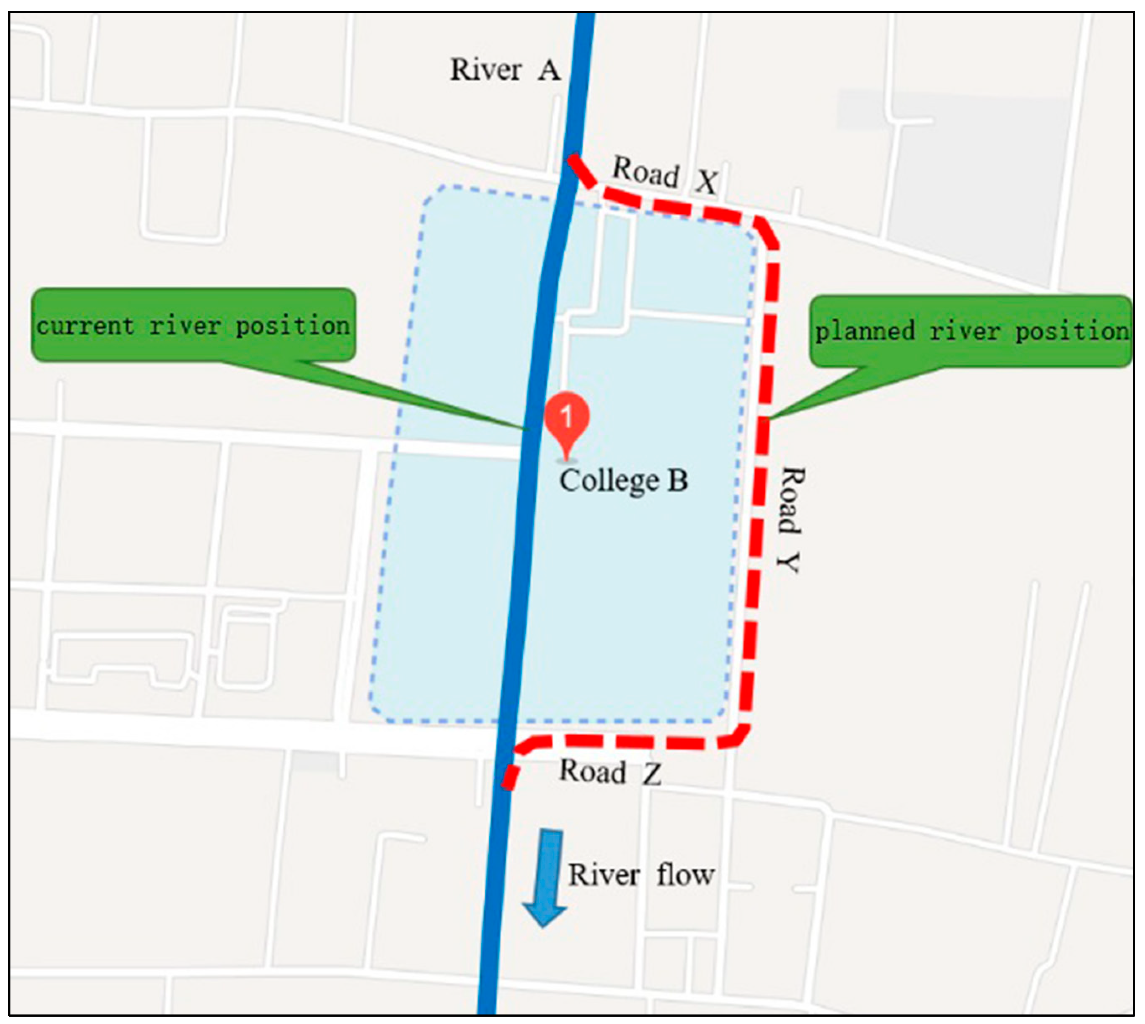
College B will be constructed near River A. There was an arrangement contradiction between the construction location of College B and the current route of River A. In order to ensure the construction of College B and the flood control in the river, after discussion, the related departments finally decided to reroute the river as follows (see Figure 1):
(1) Excavate concrete-lined 3-channel culverts (each channel of the culverts has a 3500 × 2500 mm2 rectangular cross section, with a bottom longitudinal slope of 0.001), along the south side of Road X, the west side of Road Y, and the north side of Road Z; reroute River A to the east side of College B, and merge the new river course into the downstream of current River A on the south side of College B.
(2) In order to facilitate dredging, every 100 m along the culverts, arrange a concrete-lined open channel that has a rectangular section, with a length of 30 m, a width of 12 m, a depth of 2.5 m and a bottom longitudinal slope of 0.001.
(3) Arrange a transition stretch (horn mouth stretch 1) at the junction of River A and Road X, with a length of 110 m, a top section width changing from 30 m to 12 m, a bottom section width changing from 18 m to 12 m, a depth changing from 3.0 m to 2.5 m, and a longitudinal slope of 0.001; arrange another transition stretch (horn mouth stretch 2) at the junction of River A and Road Z, with a length of 110 m, a top section width changing from 12 m to 30 m, a bottom section width changing from 12 m to 18 m, a depth changing from 2.5 m to 3.0 m, and a bottom longitudinal slope of 0.001. The two transition stretches shall both be lined with ecological revetment, and the cross section schematic diagram is shown in Figure S1.
(4) The planned cross sections upstream of the junction of River A and Road X and downstream of the junction of River A and Road Z are both trapezoidal with ecological protection, and the two river stretches are both planned to have a top width of 30 m, a bottom width of 18 m, a depth of 3.0 m, a slope coefficient of 2 and a bottom longitudinal slope of 0.001.
(5) The total length of the rerouted stretch of River A is about 1300 m and the planned design standard is for once-in-20-years floods. The planned river flow rate for once-in-20-years floods is 29.4 m3/s, and the planned river flow rate for once-in-50-years floods is 34.5 m3/s.
It is generally believed that the river flow is steady uniform flow for a single cross section of the urban river course, which greatly simplifies the hydraulic calculation work. In the practical urban river course planning and designing, the rationality and feasibility of the planning scheme with the model method (unsteady flow) are rarely verified because of the shortage of model funding and the limitation of the project cycle. However, the planned cross sections in River A are complex and diverse, and there are four right-angle turns and several alternately-arranged culverts and open channels in River A’s rerouted area, which lead to backwater, erosion and water depth difference between the two sides of the river. Hence, the change rules of the hydraulic factors of the river course cannot be predicted accurately using a conventional urban river course planning method (steady uniform flow). Therefore, in order to analyze the flow characteristics of the river more clearly and accurately in this study, River A was divided into four stretches and each stretch was discussed and analyzed separately with the MIKE21 FM model. Based on the analysis and summary of flow characteristics of the river course with complex cross sections, it provides technical support and practical experience for the successful completion of the subsequent similar planning and designing work.
2.2. Model Description
The MIKE21 FM model is a 2D shallow water equation based on numerical solutions and an incompressible Reynolds-averaged Navier–Stokes Equation integrated along the water depth (see Formulas 1–4) [31]. Therefore, the model integrates continuity, momentum, temperature, salinity and density equations, which can use the Cartesian coordinates or spherical coordinates to simulate changes of water level and flow due to various acting forces and any 2D free surface flow without considering stratification, by using unstructured grids on a plane [31].
where , and are the Cartesian co-ordinates in m; and are the velocity components in the x and y direction in m/s; is the time in s; is the bottom elevation in m; is depth of water in m; = + is the total water depth in m; , are the velocity components in the x and y direction in m/s; is the gravitational acceleration in m/s2; = 2Ωsinφ is the Coriolis parameter (Ω is the angular rate of revolution and φ is the geographic latitude) in s−1; is the density of water in kg/m3; is the reference density of water in kg/m3; , , and are components of the radiation stress tensor in kg/s2; and are the surface stress in kg/s2m; and are the bottom stress in kg/s2m; is atmospheric pressure in kg/s2m; is the magnitude of the discharge due to point sources in s−1; and are the velocity by which the water is discharged into the ambient water in m/s; , and are the lateral stresses in m2/s2, which are estimated using an eddy viscosity formulation based on the depth average velocity gradients:
where A is the horizontal eddy viscosity in m2/s; is a constant, which should be chosen within the range from 0.25 to 1.0; is a characteristic length in m.
The numerical calculation method used in the MIKE21 FM model is the finite volume method in cells [32,33]. The finite volume method is to divide a continuous body into triangle and quadrilateral non-overlapping cells. The normal vector can be obtained by establishing a cell hydraulic model in the outer normal direction and solving the one-dimensional Riemann problem. This method has a good property of integral conservation and can be used to handle supercritical flows and discontinuous solutions accurately.
The numerical calculation accuracy of the MIKE21 FM model is becoming more and more recognized. Gayer et al., simulated the influence of eddy current and roughness coefficient in the tsunami model with the MIKE21 FM model, and the calculated results were nicely consistent with the measured data [34]; Sokolov et al., carried out a simulation analysis with the measured data of the Baltic Sea collected by the Polish Academy of Sciences and found out that the correlation between the simulation results and the measured results was up to 0.86 [35]; Pedersen et al., carried out a simulation analysis with the measured tsunami data along the northern coast of Sumatra and found out that the simulation results were basically consistent with the measured data after several times of debugging [36]. Xie et al., determined the model parameters based on flooding data of the Luanhe River measured in 2012 to make the simulated flood level agree well with the measured flood level hydrograph [37]. Feng et al., elaborated the modeling process of the ocean flow field in simulation with the MIKE21 FM module and found that the measured results and the simulation results matched within an allowable error range for model verification [38]. Guo et al., simulated the flood evolution of the Pajiang River flood storage area, and demonstrated that the MIKE21 FM model had high simulation accuracy and credible simulation results, which could be used for numerical simulation of floods in more complex flood storage areas [39].
2.3. Calculation Conditions
2.3.1. Model Parameters
River A is proposed to be rerouted, and there are currently no measured data and similar planning data for reference. In order to do it in a scientific and accurate way, the selection of model parameters in this study was conducted based on relevant references published by domestic and foreign researchers [34,35,36,37,38,39,40]. On the other hand, relevant model parameters (see Table 1) were determined by considering the actual conditions of the project and the engineering safety. At the same time, considering the complex cross sections and various structures along the river course, in order to avoid the setting of model parameters this study described the relevant complex cross sections and structures in the actual terrain as much as possible, which can improve the accuracy of numerical calculation; for example, the local terrain correction methods [38] were selected to describe the 3-channel culverts and the transition stretches in the digital elevation model, to avoid setting related parameters such as the water head loss coefficient and the diffusion coefficient.
For roughness coefficients, relevant hydraulic studies were referred to [41] (see Table 2). The roughness coefficient of the trapezoidal stretches with ecological revetment was taken as 0.025 and the roughness coefficient of the concrete-lined 3-channel culverts was taken as 0.017.
There are still no mature methods for selecting roughness coefficients. If the roughness coefficient value is too small, the water flow resistance may be underestimated and the drainage capacity of the proposed river course may be overestimated, which may result in overflow and other disasters [41].
2.3.2. Terrain Processing and Meshing
Terrain processing and meshing are important and challenging technical issues in the simulation analysis. Terrain data are the basic data for the model. The quality of the terrain data directly determines the reliability of the model’s results. There are complex cross sections in the planned river course, which need to be described in the terrain. Therefore, there are high requirements for the fineness of the terrain. Based on the previous modeling experiences and related references [42], particular attention should be paid to the effects of terrain interpolation in areas with large terrain fluctuations. According to the planned river, the terrains should be specially treated at the junctions of the side slope to the river bottom, culverts, open channels and transition stretches.
At the same time, the areas with significantly changing terrain elevation should be meshed separately to avoid divergence in the model calculation. It should be noted that the solution to this terrain was completely based on the section size and elevation of the river section (see Figure S2), so as to predict actual flow characteristics of the planned River A in a more scientific and accurate way.
2.3.3. Boundary Conditions
Two boundary conditions needed to be set in this project: the water level boundary condition and the flow rate boundary condition. The water level boundary was set at about 840 m in the downstream away from the junction of River A to Road Z, and the flow rate boundary was set at about 540 m in the upstream away from the junction of River A to Road X. The specific values should be based on different simulation scenarios (see Section 2.4).
2.4. Scenario Settings
In order to simulate and analyze the changes of hydraulic factors in River A in a better way, this study set four simulation scenarios (see Table 3). The simulation scenarios 1 and 2 are planned design working conditions that are used to analyze and summarize the changes of hydraulic factors, propose pointed opinions on planning and verify the rationality of the planned river course further, to provide a scientific basis for river planning. The simulation scenario 3 is check and comparison working conditions that are used to simulate and analyze the changes of the hydraulic factors in the culvert and those in other river stretches due to the changes of the roughness coefficient in this stretch, when the culvert’s clogging leads to an increase in the roughness coefficient. Furthermore, based on the results obtained with simulation scenario 3, targeted suggestions for follow-up management of the river can be proposed, to ensure successful implementation of the long-term river pollution control system of China [43,44]. The simulation scenario 4 is design check working conditions that are used to simulate and analyze the changes of the hydraulic factors in the river when the whole stretch of the river is concrete-lined, which can provide a scientific basis for the comparison and selection of river planning schemes.
3. Results and Discussion
Based on the simulation results, and taking into account the influence of backwater in the river, from the downstream to the upstream of the river, the downstream trapezoidal stretch, the transition stretch (horn mouth stretch 2), the culvert and the open channel stretch, the upstream stretch (horn mouth stretch 1 and the upstream trapezoidal stretch).
3.1. Downstream Trapezoidal Stretch
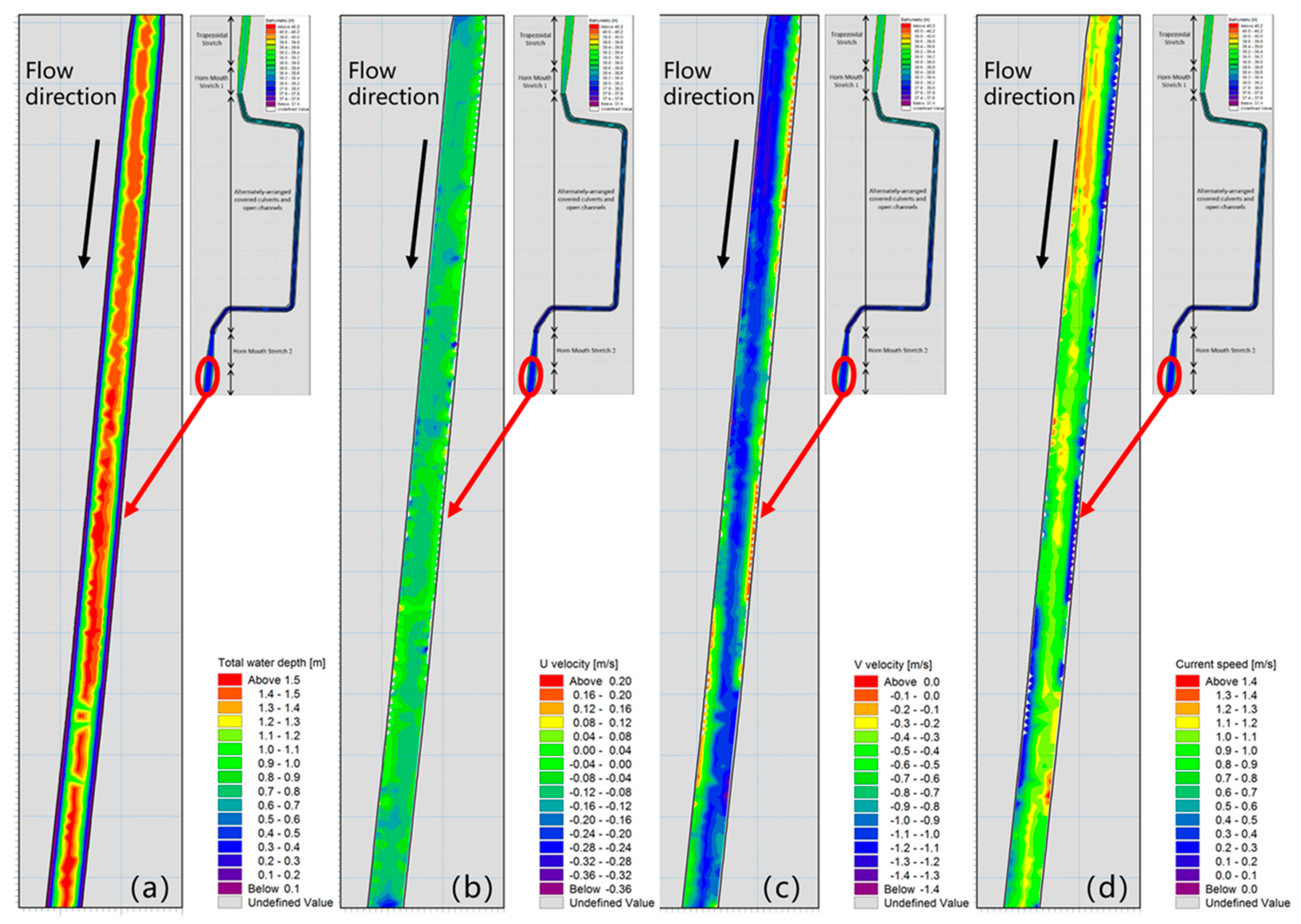
(1) According to the simulation results of Scenario 1, the water depth and flow velocity of the downstream trapezoidal stretch are clarified as Figure 2. As shown in Figure 2a, the upstream water depth of the bottom is lower than that in the downstream and the water depth at the bottom of the river is higher than the water depth on both sides in a single cross section (see Figure S3); the water depth on the right side averages 0.61 m and changes within the range from 0~1.26 m; the water depth on the left side averages 0.83 m and changes within the range from 0~1.57 m; the water depth at the bottom of the river averages 1.45 m and changes within the range from 0.90~1.57 m.
As shown in Figure 2b, the flow velocity on the right side averages −0.08 m/s and changes within the range from −0.26~0.19 m/s; the flow velocity on the left side averages −0.07 m/s and changes within the range from −0.40~0.19 m/s; the flow velocity at the bottom of the river averages −0.09 m/s and changes within the range from −0.37~0.14 m/s.
As shown in Figure 2c, the flow velocity on the right side is larger than that on the left side in a single cross section in the upstream, while the flow velocity on the left side is larger than that on the right side in a single cross section in the downstream. The flow velocity on the right side averages −0.72 m/s and changes within the range from −1.52~0 m/s; the flow velocity on the left side averages −0.73 m/s and changes within the range from −1.48~0 m/s; the flow velocity at the bottom of the river averages −1.0 m/s and changes within the range from −1.31~0 m/s.
As shown in Figure 2d, the current flow velocity on the right side (the current flow velocity is the combination of the horizontal flow velocity and the vertical flow velocity) is greater than that on the left side in a single cross section in the upstream, while the flow velocity on the left side is greater than that on the right side in a single cross section in the downstream; the flow velocity on the right side averages 0.73 m/s and changes within the range from 0~1.54 m/s; the flow velocity on the left side averages 0.73 m/s and changes within the range from 0~1.47 m/s; the flow velocity at the bottom of the river averages 1.0 m/s and changes within the range from 0.07~1.33 m/s.
From the above results, it can be seen that the water depth in the downstream trapezoidal stretch gradually increases from upstream to downstream, and the maximum water depth at the bottom of the river is 1.57 m. The planned water depth in this stretch is 3 m. Therefore, the water depth meets the planning requirement of the design standard for once-in-20-years floods; the flow velocity of the river does not vary dramatically, and the average flow velocity at the bottom of the river is 1.0 m/s, which meets the flow velocity requirement. The Froude number is about 0.3, which indicates that the flow is slow and meets the planning requirements; the average water depth on the right side of the river is lower than that on the left side, which leads to horizontal circulation in the river, thus causing a water depth difference of about 0.22 m between the two sides of the river. The water depth difference is below the designed safe super elevation and meets the planning requirements; there are some flow velocity differences between the upstream and downstream, and between the left and right sides of the river. In the next design stage, local bank reinforcement on the right side in the upstream and on the left side in the downstream should be considered, to prevent local erosion and deposition in the river.
(2) Simulation scenario 2 was analyzed in the same way. The variations of the hydraulic factors in the downstream trapezoidal stretch were basically the same as those in scenario 1 (see Figure S4).
Based on the statistical analysis, the water depth in the downstream trapezoidal stretch gradually increases from upstream to downstream, and the maximum water depth at the bottom of the river is 1.71 m. The planned river depth in this stretch is 3 m. Therefore, the water depth meets the planning requirement that no overflow occurs in once-in-50-years rains. The average water depth on the right side is about 0.18 m lower than that on the left side. The water depth difference in this scenario is lower than that in scenario 1. This is mainly because the dominant effect of vertical flow velocity in scenario 2 is stronger than that in scenario 1, thus weakening the vertical circulation effect of the river.
(3) The simulation conditions of the downstream trapezoidal stretch in scenario 3 are the same as those in scenario 2, but different from those on the upstream culverts. According to the above analysis, the water flow in the entire stretch is slow, so the hydraulic conditions in the downstream trapezoidal stretch are not affected by the changes in the hydraulic conditions of the upstream culvert, which will not be analyzed in this study.
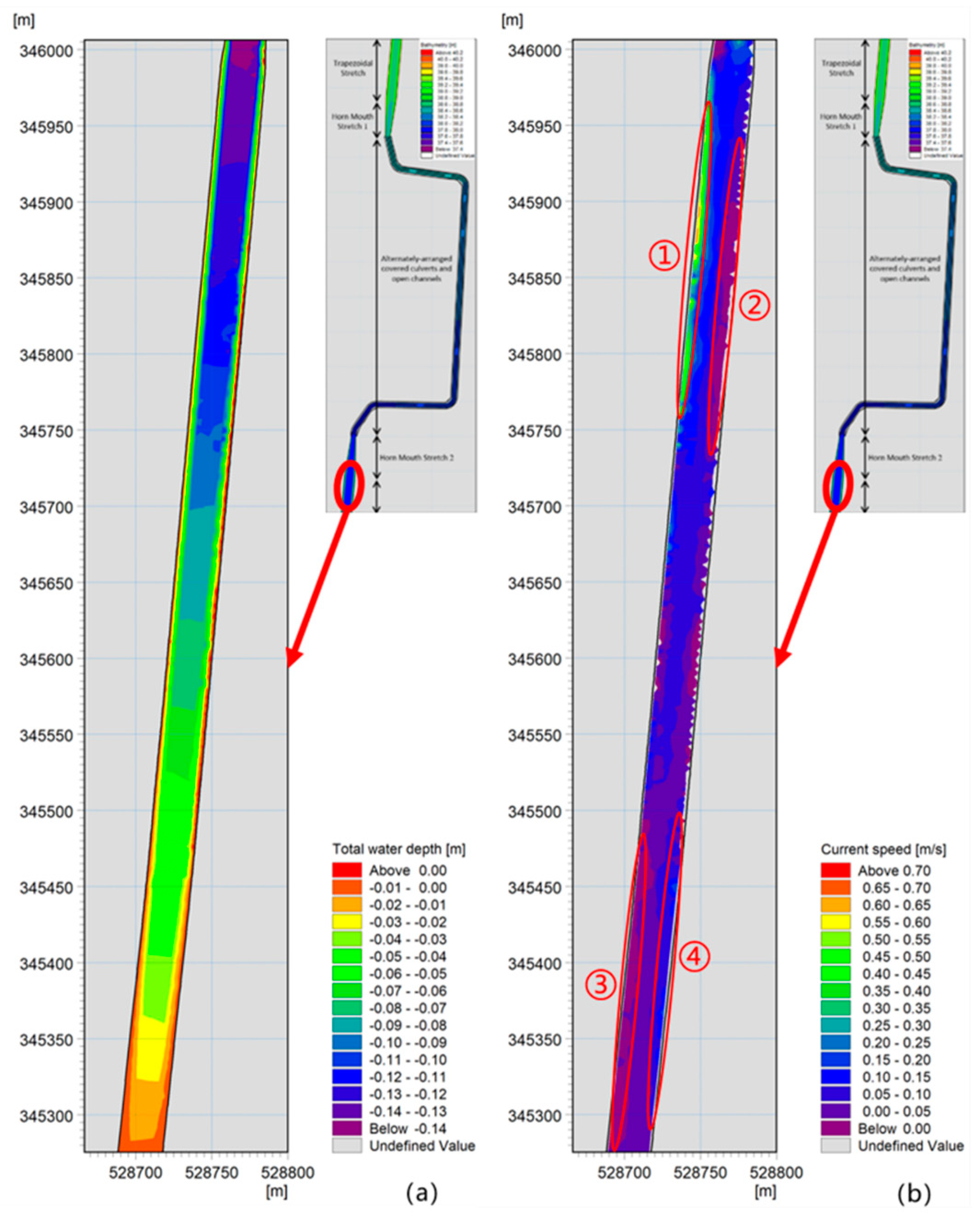
(4) The comparison of the simulation results between scenario 4 and scenario 2 is shown in Figure 3. The water depth difference in the downstream trapezoidal stretch changes within the range from −0.14~0 m. The current flow velocity difference changes within the range from 0~0.75 m/s. The local flow velocity difference is less than 0 m/s.
By analysis, it can be seen that the roughness coefficient in this stretch decreases from 0.025 to 0.017, which means that the ecological revetment in the river’s planned section is replaced by concrete revetment. The current flow velocity in the river increases but the water depth decreases, as shown in Figure 3. The water depth difference, as shown in Figure 3a, increases gradually from upstream to downstream, until it increases to 0 m/s at the downstream water level boundary and the maximum water depth decreases by 0.14 m. In Figure 3b, the current flow velocity difference between the two locations ② and ③ is less than 0 m/s, but the current flow velocity difference between the two locations ① and ④ is relatively larger, which indicates that the dredging of the river stretch at ② and ③ should be improved and that the river revetment of the river stretch at ① and ④ should be strengthened.
3.2. Transition Stretch (Horn Mouth Stretch 2).
(1) Based on the simulation results of scenario 1, the water depth and flow velocity results in the transition stretch are shown in Figure S5.
As shown in Figure S5a, the water depth at the bottom of the river from upstream to downstream first decreases and then increases. The water depth at the bottom of the river is higher than that at the both sides in a single cross section (see Figure S6); the water depth on the right side averages 0.53 m and changes within the range from 0~1.33 m; the water depth on the left side averages 0.47 m and changes within the range from 0~1.11 m; the water depth at the bottom of the river averages 1.40 m and changes within the range from 1.30~1.50 m.
From the results shown in Figure S5b, it can be seen that the flow velocity at the bottom of the river is greater than that on both sides in a single cross section; the flow velocity on the right side averages −0.14 m/s and changes within the range from −0.27~0.45 m/s; the flow velocity on the left side averages −0.19 m/s and changes within the range from −1.26~0.30 m/s; the flow velocity at the bottom of the river averages −0.17 m/s and changes within the range from −0.85~0 m/s.
From the results shown in Figure S5c, it can be seen that the flow velocity at the bottom of the river is greater than that on both sides in a single cross section; the flow velocity on the right side averages −0.75 m/s and changes within the range from −2.25~0 m/s; the flow velocity on the left side averages −0.55 m/s and changes within the range from −1.48~0 m/s; the flow velocity at the bottom of the river averages −1.77 m/s and changes within the range from −2.82~−0.83 m/s.
From the results shown in Figure S5, it can be seen that the current flow velocity distribution in the transition stretch is as follows: the flow velocity at the bottom of the river gradually decreases from upstream to downstream, and the flow velocity at the bottom of the river is higher than that on the both sides (see Figure S7); the flow velocity on the right side averages 0.77 m/s and changes within the range from 0~2.31 m/s; the flow velocity on the left side averages 0.60 m/s and changes within the range from 0~1.85 m/s; the flow velocity at the bottom of the river averages 1.78 m/s and changes within the range from 0.84~2.83 m/s.
According to the results above, the water depth in the transition stretch from upstream to downstream first decreases and then increases. It is because the gradually growing cross sections of the transition stretch cause a decrease in flow velocity (see Figure S7a). In the beginning, the water depth in the stretch decreases; when the water depth of the transition stretch reaches 1.38 m, backwater in the transition stretch occurs due to the backwater effect of the downstream trapezoidal stretch and the water depth increases. The level and length of the backwater are about 0.04 m and 60 m, respectively (see Figure S6a); the maximum water depth at the bottom of the river is 1.50 m. The planned water depth in this stretch is 3 m. Therefore, the water depth meets the planning requirement of design standard for once-in-20-years floods. The average water depth on the right side of the river is 0.06 m higher than that on the left side, and the difference is below the design safe super elevation and meets the planning requirement.
(2) Simulation scenario 2 was analyzed in the same way, and the changes of hydraulic factors in the downstream trapezoidal stretch were basically the same as those in scenario 1 (see Figure S8).
According to the results above, from upstream to downstream, the water depth at the bottom of the river in the transition stretch first decreases and then increases and the maximum water depth at the bottom of the river is 1.79 m. The planned water depth in this stretch is 3 m. Therefore, the water depth meets the planning requirements that no overflow occurs in once-in-50-years rains; the average water depth on the right side of the river is about 0.05 m higher than that on the left side and the water depth difference under this scenario is still lower than that in scenario 1; the maximum flow velocity in this stretch is 3.26 m/s. Concrete revetment rather than ecological grass revetment should be adopted for the section lining.
(3) Compared to scenario 2, the simulation conditions in the transition stretch in scenario 3 are similar, so the basic hydraulic conditions in the transition stretch are not affected by the changes of hydraulic conditions in the upstream culverts, which will not be analyzed in this study.
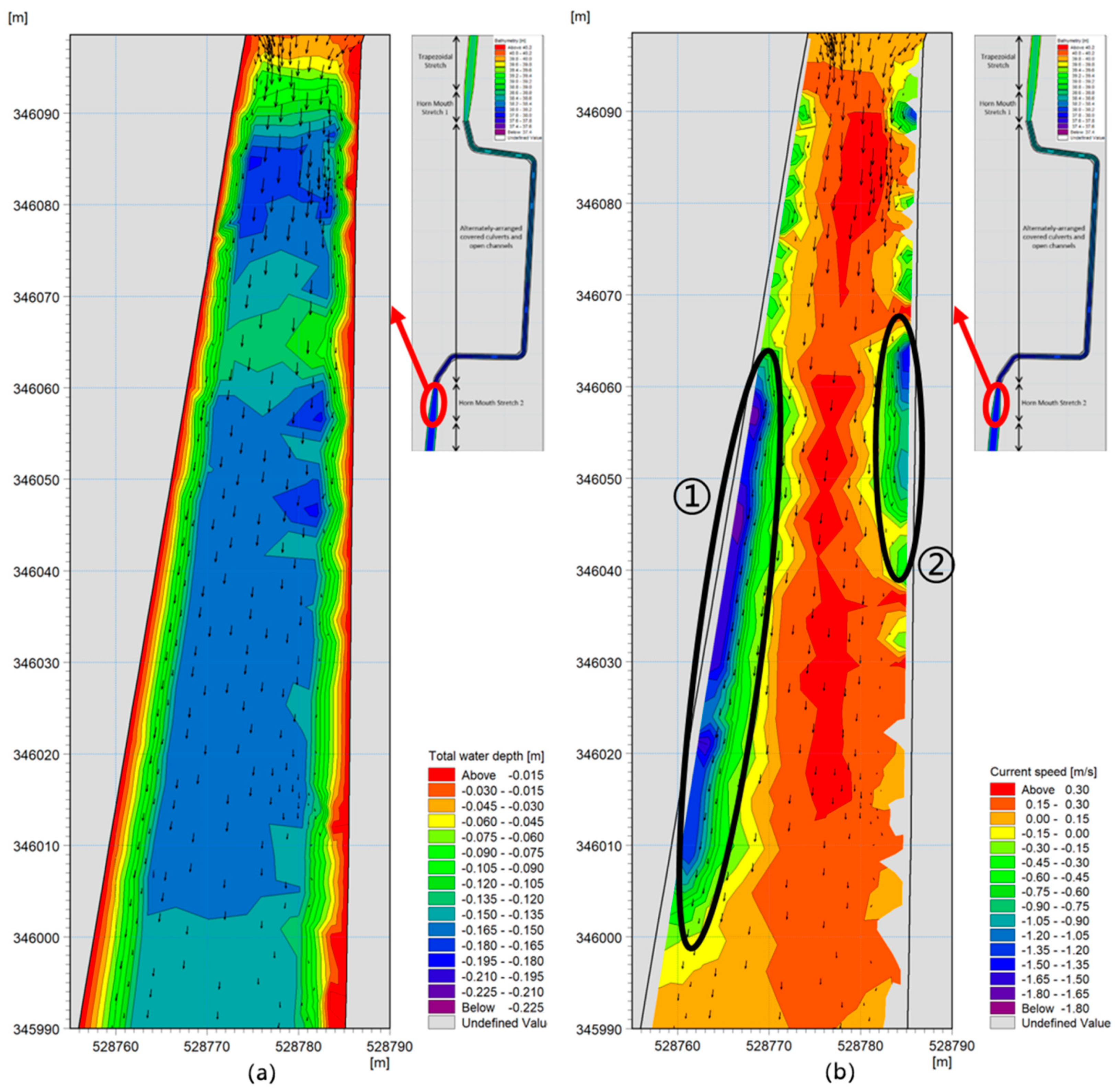
(4) The comparison of the simulation results between scenarios 4 and 2 is shown in Figure 4. The water depth difference in the transition stretch changes within the range from −0.23~−0.11 m, the current flow velocity difference changes within the range from 0~0.43 m/s and the local current flow velocity difference changes within the range from −1.8~0 m/s.
By analysis, it can be seen that due to the roughness coefficient in this stretch decreasing from 0.025 to 0.017, the current flow velocity increases, the water depth decreases and the water depth and flow velocity at a single position change in opposite directions (shown in Figure S9). The water depth decreases by 0.23 m at maximum in Figure S9a, and the current flow velocity difference between ① and ② in Figure 4b is less than 0 m/s. The two locations should be managed and dredged in the future; especially in location ①, deposition will easily occur when the flow velocity changes.
3.3. Culverts and Open Channels
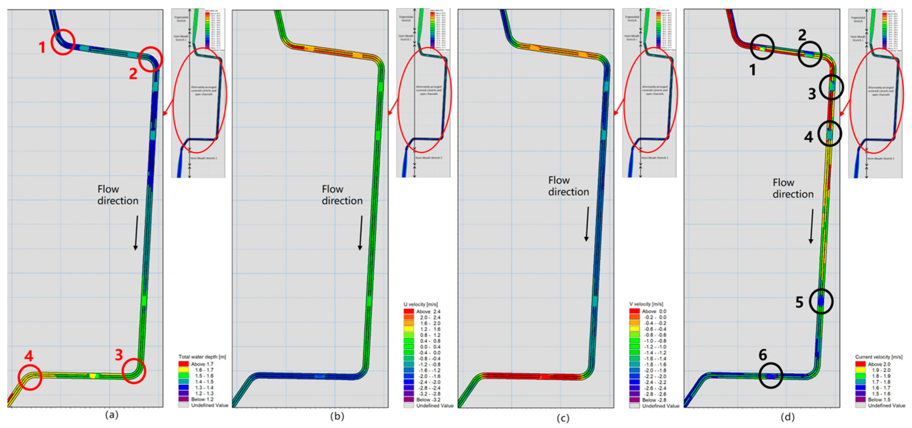
(1) Based on the simulation results of scenario 1, the water depth and flow velocity are shown in Figure 5. The four locations marked with red circles in Figure 5a are culverts and the six locations marked with black circles in Figure 5d are open channels. Because the hydraulic conditions in the sections are relatively complicated, in order to analyze in a convenient way, three channels of the culverts have been defined as the left side, middle side and right side, along the flow direction, and the water level, flow velocity and flow rate are analyzed in their vertical directions, respectively (see Figures S10 and S11).
In Figures S10 and S11, the water depth in the 3-channel culverts from upstream to downstream increases with slight fluctuation; the water depth changes within the range from 1.30~1.74 m; the height of the culverts in this stretch is 2.5 m. Therefore, the water depth meets the planning requirement of water depth of the culverts. The flow velocity in the 3-channel culverts decreases from upstream to downstream, and the flow velocity changes within the range from 1.33~2.79 m/s, which meets the planning requirements of flow velocity control. The red number represents the changes of the hydraulic factors in the turning position of the culverts, and the black number represents the changes of the hydraulic factors in the open channels, as below:
In turn 1 of the culverts, the current flow velocities in the 3 channels are in the sequence V left < V right < V middle, the water depths are in the sequence H left < H right < H middle, and the flow rates are in the sequence Q left < Q right < Q middle. The middle culvert channel in this stretch has relatively larger flow velocity and flow rate, which should be protected from scouring; the left culvert channel has lower flow velocity and flow rate, which should be dredged in time; the horizontal flow velocity (relative flow velocity between the two sides) in the culvert suddenly increases and the vertical flow velocity suddenly decreases, which indicates that the horizontal circulation effects in all culverts are enhanced and the height difference between the two sides at the turns of culvert increases.
In the open channels 1 and 2, the current flow velocity suddenly decreases. The flow velocities are in the sequence V left < V middle < V right and the flow rates are in the sequence Q left < Q middle < Q right. Therefore, dredging in the two open channels need to be enhanced, especially in the left channel of the culvert between two open channels; the current flow velocity in the open channel suddenly increases, and the average backwater level is about 0.04 m, which meets the planning requirements of safe super elevation for height.
In turn 2 of the culverts, the current flow velocities in the 3 channels are in the sequence V left < V right ≈ V middle, and the flow rates are in the sequence Q left < Q middle < Q right; therefore, in-time dredging is still necessary in the left culvert channel. The horizontal flow velocity in the section suddenly decreases and the vertical flow velocity (relative flow velocity between the both sides) suddenly increases, which indicates that the horizontal circulation effects in all culverts are enhanced and that the height difference between the two sides at the turns of culverts increases.
In the open channels 3, 4, 5 and 6, the current flow velocity suddenly decreases, the flow rate basically remain the same, and the water depth suddenly increases; the average backwater level is about 0.05m, which meets the planning requirements of safe super elevation.
In turns 3 and 4 of the culverts, the flow rates in the 3 channels are almost the same. The current flow velocities are in the sequence V right < V left ≈ V middle, and the water depths are in the sequence H middle ≈ H left < H right. Therefore, the right culvert channel needs to be dredged in time. The horizontal flow velocity (relative flow velocity between the both sides) suddenly increases, and the vertical flow velocity suddenly decreases, which indicates that the horizontal circulation effects in all culverts are enhanced and that the height difference between the two sides at the turns of culvert increases.
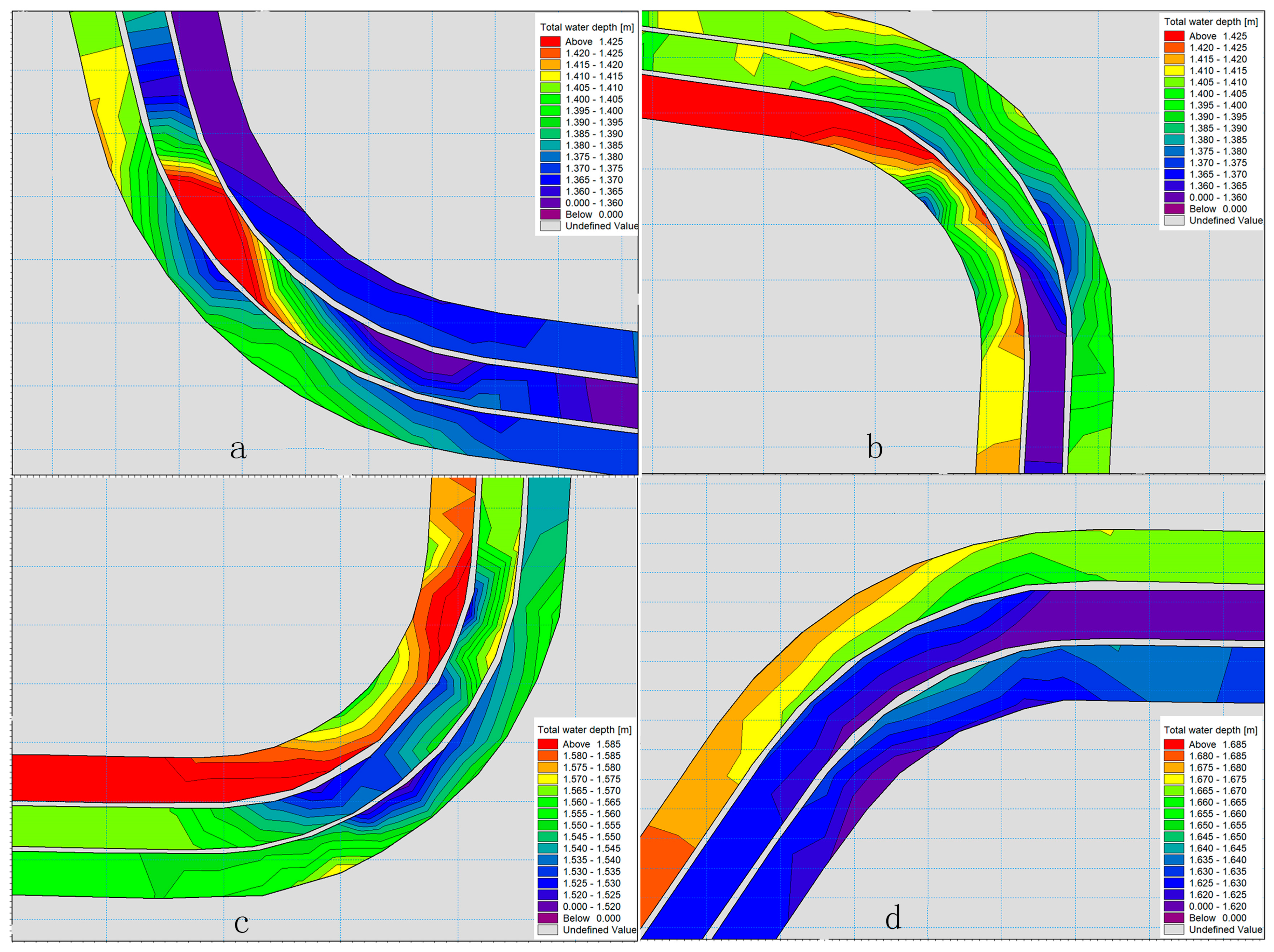
In addition, in turns 1, 2, 3, and 4 of the culverts, the water depths on the concave side are higher than those on the convex side, as shown in Figure 6.
(2) Simulation results of scenario 2 were analyzed in the same way. This study conducted analysis on the water level, flow velocity and flow rate in the vertical direction of the 3-channel culverts (see Figures S12 and S13) and the water depth map at the four turns (see Figure S14).
As shown in the figures, the water depths in the 3-channel culverts increase from upstream to downstream, changing within the range from 1.48~1.90 m. The height of the culverts in this stretch is 2.5 m. Therefore, the water depth meets the planning requirement of water depth of the culverts; the flow velocity decreases from upstream to downstream, changing within the range from 1.45~2.85 m/s, which meets the planning requirements of flow velocity control. The water depth on the concave side is higher than that on the convex side in the 3-channel culverts, and the changes of the hydraulic factors in the culverts and the open channels are also basically consistent with the results in scenario 1.
(3) The culverts should be dredged regularly in follow-up maintenance. The long-term clogging of the culverts might result in inconsistency between the actual hydraulic conditions and the planning hydraulic conditions. The local poor discharge capability in the stretch may cause overflow. Therefore, this planning compared the simulation scenario 3 with the simulation scenario 2, by changing the roughness coefficient of the culverts from 0.017 to 0.025, to predict changes of the water level, current flow velocity, and flow rate (see Figure S15).
As shown in Figure S15, the changes of the water depth, the flow velocity and the flow rate in the culverts gradually decrease from upstream to downstream; the flow velocity change in the middle culvert is the largest, with the maximum change of 0.64 m/s; the flow rate change in the left culvert is the largest, with the maximum change of 1 m/s3; and the water depth change in the 3-channel culverts basically remains the same, with the maximum change of 0.34 m and the maximum water depth of 2.24 m, Therefore, the water depth does not meet the planning requirement of the safe super elevation (at least 0.3 m). Hence, regular dredging is rather necessary. It is also shown that the setting of the six open channels is not only convenient for dredging, but also can be used to adjust the flow rate in the culverts.
(4) The simulation conditions in scenario 4 are the same as those in scenario 2, but the downstream hydraulic conditions are inconsistent. In order to study the influence of the downstream hydraulic factors on the hydraulic factors in the culverts and the open channels, this study compared the simulation results of scenarios 4 and 2 and the analysis results are shown in Figure S16.
As shown in Figure S16, the water depth, flow velocity and flow rate in the culverts do not change dramatically, the water depth difference changes within the range from −0.026~ −0.002 m, the flow velocity difference changes within the range from 0.002~0.028 m/s and the flow rate difference changes within the range from −0.013~0.006 m/s3. Therefore, when the roughness coefficient of the downstream stretch changes from 0.025 to 0.017, the water level in the culverts decreases slightly, but the flow rate, water depth and flow rate in the culverts and open channels do not change significantly. From the drainage function perspective, the concrete lining in the downstream stretch is beneficial to rapid discharge; however, from the overall appearance and return of investment perspective, this planning study still recommends the ecological slope lining for the downstream stretch.
3.4. Upstream Stretch (Horn Mouth Stretch 1 and the Upstream Trapezoidal Stretch)
(1) According to the simulation results of scenario 1, the water depth and flow velocity in the upstream stretch are shown in Figure S17. According to the results in Figure S17a, the water depth distribution at the bottom of the river first increases and then decreases from upstream to downstream (see Figure S18); the water depth on the right side averages 0.71 m and changes within the range from 0~1.72 m; the water depth on the left side averages 0.81 m and changes within the range from 0~1.31 m; the water depth at the bottom of the river averages 1.58 m and changes within the range from 0.56~1.75 m.
It can be seen from the results in Figure S17b that the horizontal flow velocity on the right side of the upstream stretch averages −0.07 m/s and changes within the range from −0.26~0.18 m/s; the horizontal flow velocity on the left side averages −0.09 m/s and changes within the range from −0.62~0.19 m/s; the horizontal flow velocity at the bottom of the river averages −0.1 m/s and changes within the range from −0.38~0 m/s.
It can be seen from the results in Figure S17c, the vertical velocity on the right side of the upstream section averages −0.73 m/s and changes within the range from −2.44~0 m/s; the vertical velocity on the left side averages −0.90 m/s and changes within the range from −2.29~0 m/s; the vertical flow velocity at the bottom of the river averages −1.1 m/s and changes within the range from −2.33~−0.47 m/s.
It can be seen from the results in Figure S17d that the current flow velocity at the bottom of the river increases from upstream to downstream (see Figure S16). The overall flow velocity on the left side is greater than that on the right side; the flow velocity on the right side averages 0.74 m/s and changes within the range from 0~2.46 m/s; the flow velocity on the left side averages 0.91 m/s and changes within the range from 0~2.30 m/s; the flow velocity at the bottom of the river averages 1.1 m/s and changes within the range from 0.47~2.35 m/s.
It can be seen from the above results that the water depth at the bottom of the river in this stretch first increases and then decreases from upstream to downstream. It is because the section area at the horn mouth stretch decreases, which results in a sudden increase in the current flow velocity and decrease in the water depth; because the water depth is affected by horn mouth stretch 1 and the downstream stretch, backwater with a level of about 0.27 m and a length of about 420 m is generated in the upstream trapezoidal stretch (see Figure S18). The water depth at the bottom of the river is 1.75 m at maximum and the planned water depth in this stretch is 3 m, which meets the planning requirements to endure once-in-20-years floods. The average horizontal flow velocity (relative flow velocity between the both sides) is less than 0, which indicates that the horizontal flow flows from left to right. The horizontal circulation in the cross section results in a water depth difference of about 0.1 m between the two sides, which meets the planning requirements of safe super elevation; at the same time, the flow rate on the left side is larger than on the right side. Therefore, deposition can easily form on the right side, which needs in-time dredging.
(2) Simulation scenario 2 was analyzed in the same way. The changes of hydraulic factors in the upstream stretch are similar to those in scenario 1 (see Figure S19).
Based on the analysis, in the upstream stretch, the water depth increases first and then decreases from the upstream to the downstream. The maximum water depth at the bottom of the river is 1.91 m and the planned water depth is 3 m. Therefore, water depth meets the planning requirement of design standard for once-in-50-year floods. The average water depth on the right side is about 0.02 m higher than that on left side, and the water depth difference in the scenario is still lower than that in scenario 1.
(3) The simulation conditions in this stretch for scenarios 3 and 2 are the same, but the downstream hydraulic conditions are inconsistent. In order to study the influence of the downstream hydraulic factors on the hydraulic factors in this stretch, this study compared simulation results in scenario 3 with those in scenario 2. The analysis results are shown in Figure S20.
As shown in the figure above, the water depth difference in the upstream section changes within the range from 0~0.24 m, the maximum water depth at the bottom of the river is 2.15 m, the horizontal flow velocity difference changes within the range from 0~0.04 m/s, the average vertical velocity difference mainly changes within the range from 0~0.30 m/s, and the current flow velocity difference mainly changes within the range from −0.35~0 m/s. The clogging of the downstream culverts might increase the risk of deposition in the upstream stretch. Therefore, the river planning should be studied as a whole, and the river management should not only strengthen the management of this stretch but also pay attention to the dredging of the downstream trapezoidal stretch.
(4) The comparison of simulation results between scenarios 4 and 2 is shown in Figure S21. The water depth difference in the upstream section changes within the range from –0.1~0 m, the maximum water depth at the bottom of the river is 1.81 m, the horizontal flow velocity difference mainly changes within the range from −0.002~0 m/s, the average vertical flow velocity difference mainly changes within the range from −0.18~0 m/s, and the current flow velocity difference mainly changes within the range from 0.01~0.20 m/s.
By analysis, due to the roughness coefficient in the section decreasing from 0.025 to 0.017, the current flow velocity in the section increases and the water depth decreases. The water depth and flow velocity in a single location change reversely, which may facilitate the discharge of the river. Therefore, the concrete revetment and ecological revetment for the stretch both meet the planning requirements. From the perspective of landscape ecology and return of investment, this planning still recommends the ecological revetment.
4. Conclusions
In this study, the planned river course was divided into four stretches for separate analysis and discussion. Each stretch has its own unique characteristics, and the change rules of hydraulic factors also vary from stretch to stretch. Based on a summary of the rules and feasibility verification of the planning scheme, this study proposed some suggestions and improvement measures for planning (see Section 3.1, Section 3.2, Section 3.3 and Section 3.4).
For River A, the main suggestions and guidance for follow-up river planning can be summarized as follows:
(1) The simulation scenarios 1 and 2 are used to analyze and summarize the changes of hydraulic factors, propose pointed opinions on planning, and further verify the rationality of the planned river course, which provides a scientific basis for river planning. Based on the analysis of the rationality and feasibility of the verified planning scheme, the planners should take pertinent measures to protect the stretches that are prone to erosion and deposition and water level differences at turns. At the same time, the river sections with excessive velocity call for revetment. On this basis, similar planning projects in the future can be quickly responded to and the planners can take measures to prevent these issues. Meanwhile for rivers with other cross section forms, it can provide useful know-how and guide the planners in the future.
(2) The simulation scenarios 3 and 4 are used to simulate and analyze the changes of the hydraulic factors in the culvert and those in other river stretches due to the changes of the roughness coefficient in this stretch. For the downstream trapezoidal stretch and upstream trapezoidal stretch and transition stretch, the roughness coefficient in this stretch decreases from 0.025 to 0.017, which means that the ecological revetment in the river’s planned section is replaced by concrete revetment. The current flow velocity in the river increases, but the water depth decreases, and the local velocity of the river decreases. For culverts and open channels, the roughness coefficient in this stretch increases from 0.017 to 0.025. The current flow velocity in the river decreases, but the water depth increases, and the water depth cannot meet the planning requirement of the safe super elevation (at least 0.3 m). Hence, regular dredging is rather necessary to ensure constancy of the roughness coefficient, and culverts should not be designed where open channels can be designed. For the upstream trapezoidal stretch, the clogging of the downstream culverts might increase the risk of deposition in the upstream trapezoidal stretch. Therefore, the river planning should be studied as a whole, and the river managers should not only strengthen the management of this stretch but also pay attention to the dredging of the downstream stretch.
Therefore, in the follow-up river planning, we should consider the overall situation, and not only pay attention to the study and analysis of the hydraulic factors of the planned river, but also pay attention to the dredging and management of the downstream river, and we should consider the changes of the hydraulic factors in the river stretches due to the changes of the roughness coefficient in this stretch.
At the same time, on the basis of this river planning research, the general rules of hydraulic factors in a river course with complex cross sections can be summarized as follows:
(1) In a single vertical section of the river course, water depth and current flow velocity change in the opposite directions, that is to say, when the current flow velocity changes, the water level will change reversely, causing a water depth difference in the vertical direction, thus resulting in backwater.
(2) In the trapezoidal and transition sections of a single river course, the flow velocity in the middle of the river course is greater than that on both sides, and the water depth in the middle is also greater than that on the two sides; in the rectangular section of a river course, the water depth and the flow velocity are basically the same as that on both sides; the water depth difference between the two sides is obvious at turns and the water depth on the concave side is greater than that on the convex side; at the junction between the culvert and the open channel, when the water flows from culvert to open channel its flow velocity decreases suddenly, while the water depth increases suddenly, which results in an increase in water head loss, thus resulting in backwater.
(3) The horizontal flow velocity and vertical velocity abruptly change at turns of the river course, enhancing the horizontal circulation in the river course, thus resulting in an increase in the water depth difference between the two sides of the river course.
(4) For river courses with complex cross sections, the flow characteristics should be considered as unsteady flow. When the flow is slow, the changes of hydraulic factors in the downstream stretch will affect the hydraulic factors in the upper stretch; therefore, the management of the river should not only strengthen the management of local stretch but also pay attention to the dredging of downstream stretch.
On this basis, when we analyze the hydraulic factors of a natural river course in the future, we can compare and analyze the hydraulic factors of the urban river course and natural river course, and then find more general rules of change. Further, the urban river course and natural river course have different evolution trends in the same river section. As the form of revetment is different, the erosion degree of the river on both sides is different, even if the same form of revetment can eventually lead to different evolution trends of the river due to the differences in flow, river upstream conditions and human activities. Based on the detailed research and analysis on the hydraulic factors of River A, the general rules of the urban river course are summarized, which establishes a solid foundation for understanding the genesis and evolution of the river course in the future.
Supplementary Materials
The following are available online at https://www.mdpi.com/2073-4441/12/3/761/s1: Figure S1: Transition stretch schematic diagram, Figure S2: Schematic diagram of terrain elevation and meshing, Figure S3: Water depth map in vertical and cross sections of the downstream trapezoidal stretch (simulation scenario 1), Figure S4: Hydraulic factors map of the downstream trapezoidal stretch (Simulation scenario 2), Figure S5: Hydraulic factors map in the transition stretch (simulation scenario 1), Figure S6: Water depth map in the vertical and cross sections in the transition stretch (simulation scenario 1), Figure S7: Current flow velocity in the vertical and cross sections in the transition stretch (simulation scenario 1), Figure S8: Hydraulic factors map in the transition stretch (simulation scenario 2), Figure S9: Reverse changes of water depth and flow velocity in a single position, Figure S10: Comparison of water depth and flow velocity in the left, middle and right culverts (simulation scenario 1); The cyan-blue curve represents the changes of the hydraulic factors in the left culvert, the red curve represents the changes of the hydraulic factors in the middle culvert, and the blue curve represents the changes of the hydraulic factors in the right culvert, Figure S11: Comparison of flow velocities in the left, middle and right culverts (simulation scenario 1), Figure S12: Comparison of the water level and flow velocity in the left, middle and right culvert channels (simulation scenario 2), Figure S13: Comparison of the flow rates in the left, middle and right culvert channels (simulation scenario 2), Figure S14: Enlarged water depth map at the four turns of the 3-channel culverts (simulation scenario 2), Figure S15: Comparison of hydraulic factors in scenarios 3 and 2, Figure S16: Comparison of hydraulic factors in scenarios 4 and 2, Figure S17: Hydraulic factors map in the upstream stretch (simulation scenario 1), Figure S18: Comparison of the water depth and current flow velocity in the upstream stretch (simulation scenario 1), Figure S19: Hydraulic factors map in the upstream stretch (simulation scenario 2), Figure S20: Comparison of hydraulic factors in scenarios 3 and 2, Figure S21: Comparison of hydraulic factors in scenarios 4 and 2.
Author Contributions
Q.W. performed model simulations, data analysis and wrote the manuscript; W.P. conceived and supervised the study; F.D., X.L. and N.O. helped the establishment of model and data analysis. All authors have read and agreed to the published version of the manuscript.
Funding
This study was jointly supported by the Major Science and Technology Program for Water Pollution Control and Treatment of China (2017ZX07101004-001), National Natural Science Foundation of China (51809288, 51861135314), National Key R&D Program of China (2018YFC0407702), Basic Research Program of the China Institute of Water Resources and Hydropower Research (WE0145B532017).
Conflicts of Interest
The authors declare no conflict of interest.
References
- Brookes, A.; Gregory, K.J.; Dawson, F.H. An assessment of river channelization in England and Wales. Sci. Total Environ. 1983, 27, 97–111. [Google Scholar] [CrossRef]
- Hickin, E.J. The development of meanders in natural river-channels. Am. J. Sci. 1974, 274, 414–442. [Google Scholar] [CrossRef]
- Wohl, E.; Merritts, D.J. What is a natural river? Geogr. Compass 2007, 1, 871–900. [Google Scholar] [CrossRef]
- Findlay, S.J.; Taylor, M.P. Why rehabilitate urban river systems? Area 2006, 38, 312–325. [Google Scholar] [CrossRef]
- Cardoso, A.; Graf, W.H.; Gust, G. Uniform flow in a smooth open channel. J. Hydraul. Res. 1989, 27, 603–616. [Google Scholar] [CrossRef]
- Bridge, J.S. A revised model for water flow, sediment transport, bed topography and grain size sorting in natural river bends. Water Resour. Res. 1992, 28, 999–1013. [Google Scholar] [CrossRef]
- Darby, S.E.; Alabyan, A.M.; Van de Wiel, M. Numerical simulation of bank erosion and channel migration in meandering rivers. Water Resour. Res. 2002, 38, 1163–1186. [Google Scholar] [CrossRef]
- Zhang, M. Study on the Hydrodynamic and Water Quality Model in River. Ph.D. Thesis, Dalian University of Technology, Dalian, China, 2007. [Google Scholar]
- Liu, X. Gravel Bed-Load Transport and its Modelling. Ph.D. Thesis, Sichuan University, Chengdu, China, 2004. [Google Scholar]
- Xia, R. Relation between mean and maximum velocities in a natural river. J. Hydraul. Eng. 1997, 123, 720–723. [Google Scholar] [CrossRef]
- Lane, S.; Bradbrook, K.; Richards, K.; Biron, P.; Roy, A. The application of computational fluid dynamics to natural river channels: Three-dimensional versus two-dimensional approaches. Geomorphology 1999, 29, 1–20. [Google Scholar] [CrossRef]
- Yu, X.; Tan, G.; Zhao, L.; Wang, J. Planar 2-D flow and sediment numerical modeling of branching river. J. Sichuan Univ. (Eng. Sci. Ed.) 2007, 39, 33–37. [Google Scholar]
- Jia, D. Three-Dimensional Numerical Simulation of Lateral Migration of Alluvial Channels with Composite Banks. Ph.D. Thesis, Tsinghua University, Beijing, China, 2010. [Google Scholar]
- Chen, X.; Wang, D.; Tian, F.; Sivapalan, M. From channelization to restoration: Sociohydrologic modeling with changing community preferences in the Kissimmee River Basin, Florida. Water Resour. Res. 2016, 52, 1227–1244. [Google Scholar] [CrossRef] [Green Version]
- Wohl, E.; Lane, S.N.; Wilcox, A.C. The science and practice of river restoration. Water Resour. Res. 2015, 51, 5974–5997. [Google Scholar] [CrossRef] [Green Version]
- Palmer, M.A.; Bernhardt, E.; Allan, J.; Lake, P.S.; Alexander, G.; Brooks, S.; Carr, J.; Clayton, S.; Dahm, C.; Follstad Shah, J. Standards for ecologically successful river restoration. J. Appl. Ecol. 2005, 42, 208–217. [Google Scholar] [CrossRef]
- Wohl, E.; Angermeier, P.L.; Bledsoe, B.; Kondolf, G.M.; MacDonnell, L.; Merritt, D.M.; Palmer, M.A.; Poff, N.L.; Tarboton, D. River restoration. Water Resour. Res. 2005, 41, W10301. [Google Scholar] [CrossRef]
- Beechie, T.; Imaki, H. Predicting natural channel patterns based on landscape and geomorphic controls in the Columbia River basin, USA. Water Resour. Res. 2014, 50, 39–57. [Google Scholar] [CrossRef]
- Garcia-Navarro, P.; Saviron, J. McCormack’s method for the numerical simulation of one-dimensional discontinuous unsteady open channel flow. J. Hydraul. Res. 1992, 30, 95–105. [Google Scholar] [CrossRef]
- Hersberger, D.S.; Franca, M.J.; Schleiss, A.J. Wall-roughness effects on flow and scouring in curved channels with gravel beds. J. Hydraul. Res. 2016, 142, 04015032. [Google Scholar] [CrossRef]
- An, M. The Numerical Simulation of the River Flow on Urban Landscape River. Master’s Thesis, North China University of Water Resources and Electric Power, Zhengzhou, China, 2016. [Google Scholar]
- Costabile, P.; Costanzo, C.; De Bartolo, S.; Gangi, F.; Macchione, F.; Tomasicchio, G.R. Hydraulic characterization of river networks based on flow patterns simulated by 2-D shallow water modeling: Scaling properties, multifractal interpretation and perspectives for channel heads detection. Water Resour. Res. 2019, 55, 7717–7752. [Google Scholar] [CrossRef]
- Williams, R.D.; Brasington, J.; Hicks, M.; Measures, R.; Rennie, C.; Vericat, D. Hydraulic validation of two-dimensional simulations of braided river flow with spatially continuous aDcp data. Water Resour. Res. 2013, 49, 5183–5205. [Google Scholar] [CrossRef] [Green Version]
- Chin, A.; Gregory, K.J. Managing urban river channel adjustments. Geomorphology 2005, 69, 28–45. [Google Scholar] [CrossRef]
- Gregory, K.J. Urban channel adjustments in a management context: An Australian example. Environ. Manag. 2002, 29, 620–633. [Google Scholar] [CrossRef] [PubMed]
- Chen, A.S.; Evans, B.; Djordjević, S.; Savić, D.A. Multi-layered coarse grid modelling in 2D urban flood simulations. J. Hydrol. 2012, 470, 1–11. [Google Scholar] [CrossRef] [Green Version]
- Uddin, M.; Alam, J.B.; Khan, Z.H.; Hasan, G.J.; Rahman, T. Two dimensional hydrodynamic modelling of Northern Bay of Bengal coastal waters. Comput. Water Energy Environ. Eng. 2014, 3, 140–151. [Google Scholar] [CrossRef] [Green Version]
- Kaergaard, K.; Fredsoe, J. Numerical modeling of shoreline undulations part 1: Constant wave climate. Coast. Eng. 2013, 75, 64–76. [Google Scholar] [CrossRef]
- Abily, M.; Duluc, C.; Faes, J.; Gourbesville, P. Performance assessment of modelling tools for high resolution runoff simulation over an industrial site. J. Hydroinform. 2013, 15, 1296–1311. [Google Scholar] [CrossRef]
- Kimiaghalam, N.; Goharrokhi, M.; Clark, S.P.; Ahmari, H. A comprehensive fluvial geomorphology study of riverbank erosion on the Red River in Winnipeg, Manitoba, Canada. J. Hydrol. 2015, 529, 1488–1498. [Google Scholar] [CrossRef]
- Yi, X. Application and Research of DHI Mike Flood Simulation Technology, 1st ed.; China Water Power Press: Beijing, China, 2014; pp. 11–253. [Google Scholar]
- Eymard, R.; Gallouët, T.; Herbin, R. Finite volume methods. Handb. Numer. Anal. 2000, 7, 713–1018. [Google Scholar]
- Barth, T.; Herbin, R.; Ohlberger, M. Finite volume methods: Foundation and analysis. In Encyclopedia of Computational Mechanics Second Edition; John Wiley & Sons: New York, NY, USA, 2018; pp. 1–60. [Google Scholar]
- Gayer, G.; Leschka, S.; Nöhren, I.; Larsen, O.; Günther, H.; Sciences, E.S. Tsunami inundation modelling based on detailed roughness maps of densely populated areas. Nat. Hazards 2010, 10, 1679–1687. [Google Scholar] [CrossRef]
- Sokolov, A.; Chubarenko, B.J.A.o.H.-E. Wind influence on the formation of nearshore currents in the Southern Baltic: Numerical modelling results. Nephron Clin. Pract. 2012, 59, 37–48. [Google Scholar] [CrossRef] [Green Version]
- Pedersen, N.H.; Rasch, P.S.; Sato, T. Modelling of the Asian tsunami off the coast of northern Sumatra. In Proceedings of the 3rd Asia-Pacific DHI Software Conference, Kuala Lumpur, Malaysia, 21–22 February 2015. [Google Scholar]
- Xie, X. Application of MIKE21 FM in Flood Hazard Mapping-a Case Study on Luanhe Right-Bank Flood Protected Zone. Master’s Thesis, Dalian University of Technology, Dalian, China, 2016. [Google Scholar]
- Feng, J. MIKE21FMApplication of mIKE21FM Numerical Model in Environmental Impact Assessment of Ocean Engineering. Master’s Thesis, Ocean University of China, Qingdao, China, 2011. [Google Scholar]
- Guo, F.; Qu, H.; Zeng, H.; Cong, F.; Geng, X. Flood routing numerical simulation of flood storage area based on MIKE21 FM model. Int. J. Hydroelectr. Energy 2013, 31, 34–37. [Google Scholar]
- Zhang, W. A 2-D numerical simulation study on longitudinal solute transport and longitudinal dispersion coefficient. Water Resour. Res. 2011, 47, 128–136. [Google Scholar] [CrossRef]
- Ye, Z.; Wen, D. Hydraulics and Hydrology of Bridge and Culvert, 1st ed.; China Communications Press: Beijing, China, 1998; p. 87. [Google Scholar]
- Wang, Q.; Zhao, S.; Zhou, Y.; Lu, Y.; Zhou, L.; Wang, Z.; Yang, W.; Gao, L. Probe into urban drainage and waterlogging prevention plan based on modeling-case study on ShaTauKok district of Shenzhen. Water Supply Drain. 2015, 51, 34–38. [Google Scholar]
- Ren, M. The river-chief mechanism: A case study of china’s inter-departmental coordination for watershed treatment. J. Beijing Adm. Inst. 2015, 3, 25–31. [Google Scholar]
- Wang, S.; Cai, M. Critique of the system of river-leader based on the perspective of new institutional economics. China Popul. Resour. Environ. 2011, 21, 8–13. [Google Scholar]
Figure 1.
River position schematic diagram.

Figure 2.
Hydraulic factors map of the downstream trapezoidal stretch (simulation scenario 1). (a) Water depth map; (b) Horizontal flow velocity; (c) Vertical flow velocity; (d) Current flow velocity (From bottom to top and left to right, the flow velocity was set to be positive).
Figure 2.
Hydraulic factors map of the downstream trapezoidal stretch (simulation scenario 1). (a) Water depth map; (b) Horizontal flow velocity; (c) Vertical flow velocity; (d) Current flow velocity (From bottom to top and left to right, the flow velocity was set to be positive).

Figure 3.
Comparison of hydraulic factors between scenario 4 and scenario 2. (a) Water depth difference; (b) Current flow velocity difference.
Figure 3.
Comparison of hydraulic factors between scenario 4 and scenario 2. (a) Water depth difference; (b) Current flow velocity difference.

Figure 4.
Water depth differences and current flow velocity differences in scenario 4 and scenario 2. (a) Water depth difference; (b) Current flow velocity difference.
Figure 4.
Water depth differences and current flow velocity differences in scenario 4 and scenario 2. (a) Water depth difference; (b) Current flow velocity difference.

Figure 5.
Hydraulic factors map in the culverts and open channels (simulation scenario 1). (a) Water depth map; (b) Horizontal flow velocity; (c) Vertical flow velocity; (d) Current flow velocity.
Figure 5.
Hydraulic factors map in the culverts and open channels (simulation scenario 1). (a) Water depth map; (b) Horizontal flow velocity; (c) Vertical flow velocity; (d) Current flow velocity.

Figure 6.
Enlarged water depth map of the four turns of 3-channel culverts (simulation scenario 1). (a) Enlarged water depth map of the locations marked with red circles 1 in Figure 5a; (b) Enlarged water depth map of the locations marked with red circles 2 in Figure 5a; (c) Enlarged water depth map of the locations marked with red circles 3 in Figure 5a; (d) Enlarged water depth map of the locations marked with red circles 4 in Figure 5a.


Table 1.
Model parameters table [31].
Table 1.
Model parameters table [31].
| Model Parameters | Recommended Range | Module Default Value | Value in This Study |
|---|---|---|---|
| Time step | 0.01–30 s | 0.01–30 s | 0.01–0.03 s |
| Wet and dry boundaries | - | hdry = 0.005 hflood = 0.05 hwet = 0.1 | hdry = 0.01 hflood = 0.1 hwet = 0.3 |
| Manning coefficient (n) | 0.01–0.05 m1/3/s | 0.03 m1/3/s | Roughness coefficient of ecological slope section (n): 0.025; Roughness coefficient of 3-channel culverts (n): 0.017 |
| Vortex viscosity coefficient | 0.25–1.0 | 0.28 | 0.28 |
| Structures | - | - | Described in the terrain DEM |
Table 2.
Roughness coefficients table [41].
Table 2.
Roughness coefficients table [41].
| No. | Boundary TYPE and Conditions | n |
|---|---|---|
| 1 | Thoroughly planed wood boards and freshly cleaned pig iron pipes and cast-iron pipes with smooth lining and joints | 0.01 |
| 2 | Dirty water supply and drainage pipes; ordinary concrete surfaces; ordinary brickworks | 0.014 |
| 3 | Old brickworks; very rough concrete surfaces; carefully excavated smooth rock faces | 0.017 |
| 4 | Canals in solid clay; loess with continuous silt layers; well-maintained large canals in earth | 0.0225 |
| 5 | Ordinary large earth canals; well-maintained small canals in earth; natural rivers under excellent conditions | 0.025 |
| 6 | Earth drains under particularly bad conditions; natural rivers under poor conditions (with much wild grasses and stones, irregular and curved riverbeds and many collapses and deep pools, etc.) | 0.04 |
Table 3.
Simulation scenarios.
| Scenario | Roughness Coefficient | Water Level Boundary | Flow Rate Boundary |
|---|---|---|---|
| 1 | The roughness coefficient of the ecological revetment section was taken as 0.025 and the roughness coefficient of the culvert was taken as 0.017 | Water depth for once-in-20-years floods (1.46 m) | Flow rate for once-in-20-years floods (29.4 m3/s) |
| 2 | Water depth for once-in-50-years floods (1.58 m) | Flow rate for once-in-50-years floods (34.5 m3/s) | |
| 3 | 0.025 | Water depth for once-in-50-years floods | Flow rate for once-in-50-years floods |
| 4 | 0.017 | Water depth for once-in-50-years floods | Flow rate for once-in-50-years floods |
© 2020 by the authors. Licensee MDPI, Basel, Switzerland. This article is an open access article distributed under the terms and conditions of the Creative Commons Attribution (CC BY) license (http://creativecommons.org/licenses/by/4.0/).
Share and Cite
MDPI and ACS Style
Wang, Q.; Peng, W.; Dong, F.; Liu, X.; Ou, N. Simulating Flow of An Urban River Course with Complex Cross Sections Based on the MIKE21 FM Model. Water 2020, 12, 761. https://doi.org/10.3390/w12030761
AMA Style
Wang Q, Peng W, Dong F, Liu X, Ou N. Simulating Flow of An Urban River Course with Complex Cross Sections Based on the MIKE21 FM Model. Water. 2020; 12(3):761. https://doi.org/10.3390/w12030761
Chicago/Turabian StyleWang, Qianxun, Wenqi Peng, Fei Dong, Xiaobo Liu, and Nan Ou. 2020. "Simulating Flow of An Urban River Course with Complex Cross Sections Based on the MIKE21 FM Model" Water 12, no. 3: 761. https://doi.org/10.3390/w12030761
Note that from the first issue of 2016, this journal uses article numbers instead of page numbers. See further details here.