ARIMA-M: A New Model for Daily Water Consumption Prediction Based on the Autoregressive Integrated Moving Average Model and the Markov Chain Error Correction

Abstract

Water resource is considered as a significant factor in the development of regional environment and society. Water consumption prediction can provide an important decision basis for the regional water supply scheduling optimizations. According to the periodicity and randomness nature of the daily water consumption data, a Markov modified autoregressive moving average (ARIMA) model was proposed in this study. The proposed model, combined with the Markov chain, can correct the prediction error, reduce the continuous superposition of prediction error, and improve the prediction accuracy of future daily water consumption data. The daily water consumption data of different monitoring points were used to verify the effectiveness of the model, and the future water consumption was predicted in the study area. The results show that the proposed algorithm can effectively reduce the prediction error compared to the ARIMA.

1. Introduction

Water resources are considered as an important key factor for regional sustainable development in both developing and developed countries. With the development of urbanization and the improvement of people’s living standards, the demand for water supply is increasing, and the shortage of water resources is becoming more and more serious. A crisis of water scarcity occurs in many parts of the world. With the expansion of the scope and scale of the urban water supply system, the complexity of the water supply has been significantly increased. The decision-making for the water supply is only based on the experience and judgment of the current water demand, which causes difficulty in predictability of water supply, leading to excessive water supply. In addition, the excessive water supply increases the pressure on the water supply network, which increases the risk of leakage and burst of water pipes. Therefore, the analysis of urban water supply and demand is of great significance for prediction of the urban water demand. Firstly, by quota analysis of water consumption on different regions, the allocation and management of water resources in the water administration department can be optimized. Effective forecasting of water consumption is helpful in improving emergency response ability of water resource management, as well as in providing technical support for assessment or management of water resource conservation. Secondly, water consumption forecast can improve management and service quality of water supply enterprises. The water supply demand forecast can be used to ensure the demand of water supply and water pressure during various periods to improve the service quality of water supply enterprises. Because urban water needs to be pressurised and transported by the pump station, the prediction of water supply can guide the optimal operation of the pump station. Hence, the utilization of stored energy in the water supply system improves, significantly, which saves the energy costs, while ensuring a safe and stable water supply. In addition, through the forecast of water consumption, the water transported by users in different regions can be reasonably distributed, which provides a basis for the distribution of water resources in water plants and reduces the dispatching cost.

Regression analysis, exponential smoothing analysis, and Markov chain model are considered as the main traditional methods for water consumption prediction. In the regression analysis, a large amount of historical data are required for statistical analysis to establish regression equations between the dependent variables and independent variables. Yasar et al. [1] established a multivariate nonlinear regression model of the monthly average water cost, total population, atmospheric temperature, relative humidity, rainfall, sunshine time, wind speed, air pressure, and water supply to predict the water supply for the Turkish city of Adana. Brekke et al. [2] adopted the stepwise regression method to introduce the water-related variables into the model, one-by-one for urban water supply prediction, which shortened the time of water consumption trend analysis and demand analysis. Brezonik and Stadelmann [3] used regression analysis to study the relationship between stormwater runoff volumes, loads, and pollutant concentrations from watersheds in the Twin Cities metropolitan area of USA, so as to predict runoff volume for rain events. Adamowski et al. [4] established a regression model between the daily water demand and the data of the previous day’s water consumption, daily precipitation, and daily maximum temperature by using multiple linear regression analysis. The model was applied to predict the water consumption data in the city of Montreal, Canada.

Markov process is a typical stochastic process proposed by the Russian mathematician Markovian. Markov chain is a stochastic process with discrete time and state. It predicts the future value [5] through the transfer probability by current information. It is widely used in the predictions relating to the economy, meteorology, environment, and so on. Tsaur [6] used a fuzzy time series Markov chain model with an application to forecast the exchange rate between the Taiwan and U.S. dollar. Yu et al. [7] predicted the short term traffic flow on the basis of the Markov chain model. In addition, Carpinone et al. [8] applied the Markov chain to wind energy prediction. Kani and Ardehali [9] proposed a hybrid neural network and Markov chain model to predict short-term wind speed. In addition, Haan et al. [10] proposed a daily rainfall prediction model based on the Markov chain. Su et al. [11] adopted a set pair analysis and Markov chain model to predict groundwater quality, and Gagliardi et al. [12] put forward the short-term water consumption prediction method of Markov chain. The empirical results showed that the proposed forecasting model based on homogeneous Markov chain is effective. Methods, which is based on regression analysis or Markov chain, provide a poor data fitting ability. For data with large fluctuation and complex influencing factors, the prediction ability is limited.

Autoregressive integrated moving average (ARIMA) was proposed by Box and Jenkins [13] in 1976. It regards the data sequence as a random sequence, and predicts future value on the basis of analyzing the correlation between series data. The ARIMA model has the advantages of fast modeling and prediction, and is widely used in the prediction of time series data. Lippi et al. [14] analyzed the effect of the ARIMA model on traffic flow prediction. Shvartser et al. [15] used ARIMA to predict daily and monthly short-term water consumption. Mombeni et al. [16] employed ARIMA models to forecast the annual water supply in Iran by monthly water consumption data. Hao et al. [17] established an ARIMA model for the prediction of runoff and sediment in the reservoir. The model was verified by an example analysis on prediction of sediment in the Three Gorges project. Garf [18] established an ARIMA model for water temperature prediction, which was used for environmental protection of early warning. Wang et al. [19] established a river streamflow prediction and analysis model-based combing model of ARIMA, which was used to predict the daily streamflow in the upper reaches of the Yellow River. Guarnaccia et al. [20] made a prediction of short-term tank water level in urban water distribution network.

Artificial neural network has a strong nonlinear approximation ability and can be used in data prediction and other fields [21]. Bennett et al. [22] used the urban water consumption prediction model, based on artificial neural network (ANN), and used demographic, socio-economic, and water appliance stock information as an input to predict the future water consumption. Mouatadid and Adamowski [23] proposed a water consumption prediction method based on the extreme learning machine neural network. Adebiyi [24] compared the performance difference between ARIMA and the neural network model on stock price prediction. The results showed that ARIMA-based prediction results can produce a better trend of prediction results, whereas the ANN-based approach can fit the prediction details well. Similarly, Sebri [25] compared the performance of Box and Jenkins’ ARIMA model and ANN model on water consumption prediction in Tunisia, and the result indicated that the traditional Box–Jenkins method outperformed ANN estimated on raw, degraded, or deseasonalized data in terms of forecasting accuracy. Thus, it is difficult to obtain the seasonal and periodic characteristics of water consumption data by ANN, and it is easy to produce over fitting problems in the limited dataset for a strong nonlinear approximation ability [26], which reduces the prediction accuracy. Therefore, it is worth performing a further study about the ARIMA model for predicting water consumption data.

However, due to the random and volatility of water consumption data, the ARIMA model will inevitably have large errors in the prediction of non-linear non-stationary time series data, with certain trends and periodicity. In addition, the process of data acquisition is tedious, which involves many links, such as acquisition, transmission, storage, and exchange. Additionally, the integrity of the obtained data cannot be guaranteed, which greatly limits the accuracy of ARIMA model prediction.

To bridge the gap in the data modelling, this study presents a water consumption prediction model, combining the ARIMA and Markov model. On the basis of data analysis and pre-processing, the water consumption prediction was carried out on the basis of the ARIMA model. Aiming at the prediction error, this study proposes a prediction value correction method that is based on Markov chain.

2. Water Data Pre-Processing

The data pre-processing procedure includes uploading the data through the sensor of the regional data monitoring point, and then gathering the data to the data processing server to form the dataset within a certain period of time. However, due to the failure of data collection point, noise, and other factors, it is easy to have data value missing, or large, small, and other abnormal data, which greatly affects the effectiveness of data processing. Therefore, effective identification and data processing are required for further data analysis.

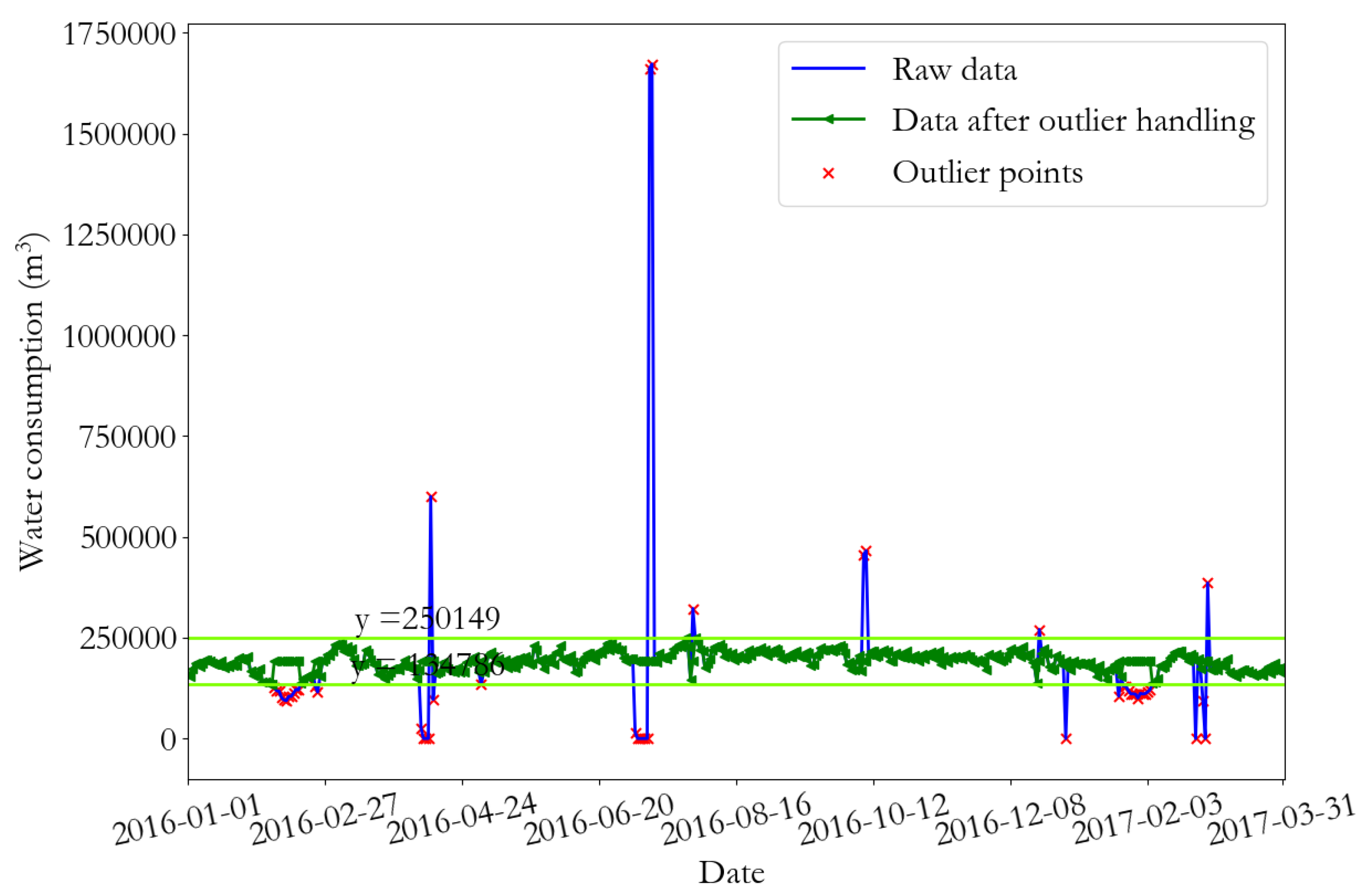
For the analysis of the collected water consumption data, the identifiable data abnormal features include data missing or zero, data mutation of zero, or a large data mutation, and so on. The above abnormal data features, zero value and missing value, can be directly tested and judged. The 3$\delta$ criterion (i.e., the pauta criterion) can be used to judge whether the mutation data is abnormally large or small. Assuming that the sample data approximately obey the normal distribution, the data contain random errors, and the error region is determined according to the probability. Furthermore, the error beyond the region is considered as gross error, and the data within the gross error range is regarded as the abnormal value. If $\delta$ is the standard deviation and $\mu$ is the mean value, the probability of data distribution in ($\mu -3\delta ,\mu +3\delta$) is 0.9973, and the data beyond this range is the abnormal value point, where $\delta$ and $\mu$ are the standard deviation and mean value, calculated from the dataset after eliminating the zero value and missing value in the water consumption data. After obtaining the abnormal data value, the data need to be recovered to obtain the normal range. Subsequently, the mean filling method is used to calculate the mean value of the dataset to remove the outliers, which include the zero value, missing value, abnormal large value, and abnormal small value, which were previously identified using the above detection method.

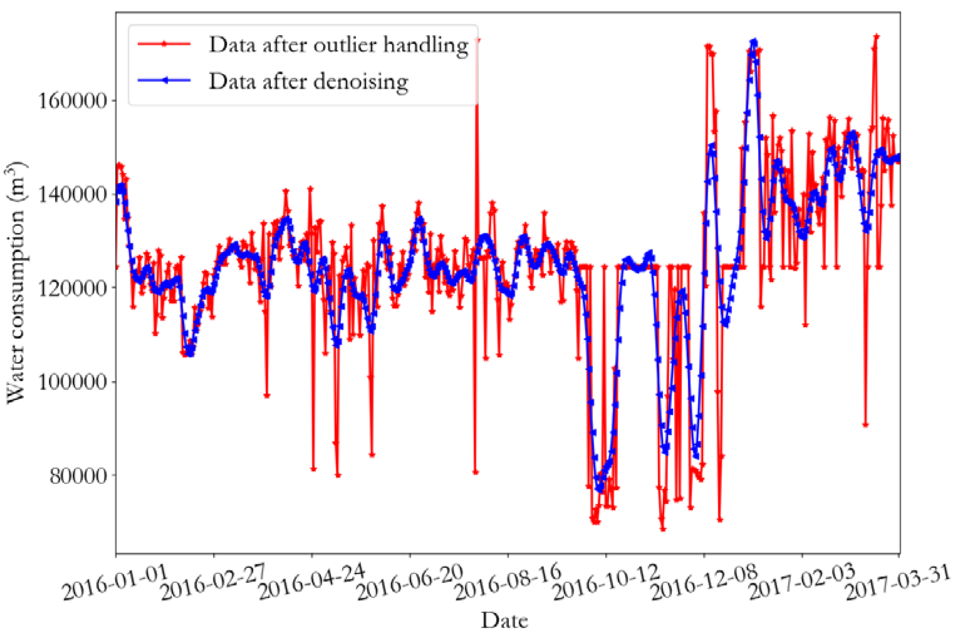
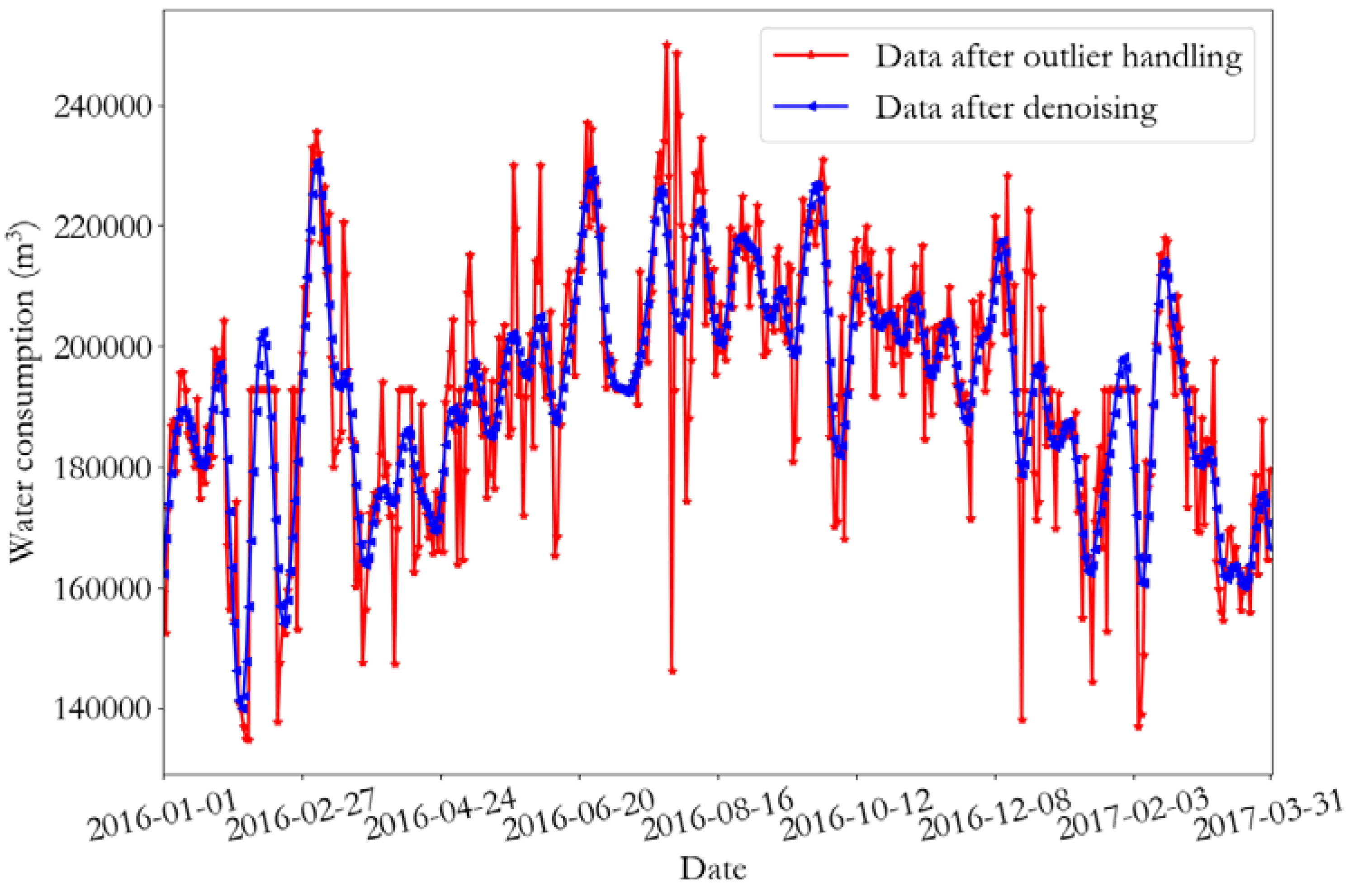
Even after the abnormal value detection and processing, the water consumption data monitoring process inevitably produces errors and noises. The use of many noise data for water consumption prediction greatly affects the data prediction, which requires further data abnormal value processing to remove data noise.

Empirical mode decomposition (EMD) is a time-frequency analysis method that can decompose time-series data into multiple intrinsic mode function (IMF) components, where each component represents a certain local feature of data. EMD has been widely used in signal de-noising, fault diagnosis, image processing, and other aspects. Using the data decomposed by the EMD, it is easy to produce mode aliasing, and different time-scale features in the IMF allow an efficient data processing [27,28]. Wu and Huang proposed the ensemble empirical mode decomposition (EEMD) method. During the decomposition process, white noise is introduced according to a certain signal-to-noise ratio, and the influence of white noise is reduced through the set average method, which has the advantage of anti-aliasing [29]. The EEMD method is used to remove the noise in the historical water consumption data. The water consumption data processed by outliers are decomposed by the EEMD to obtain N-component, including n-1 IMF component and 1 residual term r_n. The decomposed data are arranged, according to the frequency from high to low, and afterwards the highest frequency component is removed and the residual component is summed to obtain the new data as the de-noised data.

3. Prediction of Water Consumption Based on Markov Chain Modification

The daily water consumption data is nonlinear and uncertain, and interrelated to time. The daily water consumption data prediction is a time-series prediction problem. In this study, the ARIMA model was established for daily water consumption data. Furthermore, a modified Markov chain model was proposed to forecast the daily water consumption, which can reduce the error caused by the randomness nature of the water consumption data.

3.1. Prediction Model Based on ARIMA

The ARIMA model is widely used to forecast non-stationary time series data. It can be used to forecast the trend of daily water consumption data. In a model of ARIMA (p, d, q), AR is autoregressive, p is the number of regression terms, MA is the moving average, q is the number of moving average terms, and d is the difference time to make the data a stationary series. Firstly, the non-stationary historical data x_t is processed by the d difference to develop the stable historical data y_t, fitted to the ARMA (p, q) model to predict the consumption, and then the original data x_t is obtained by d times contrast difference. The ARMA model is expressed as follows:

$$y_t=c+{\varphi }_1{y}_{t-1}+\cdots +{\varphi }_p{y}_{t-p}+{\epsilon }_t+{\theta }_1{\epsilon }_{t-1}+\cdots +{\theta }_q{\epsilon }_{t-q}$$

(1)

where ${\varphi }_1,\cdots ,{\varphi }_p$ and ${\theta }_1,\cdots ,{\theta }_q$ are constant, ${\epsilon }_t$ is a white noise sequence, then the time series $y_t$ follows the (p, q) order autoregressive moving average model, which is recorded as ARMA(p, q).

When the original data sequence is non-stationary, firstly, the data is processed by the d-th difference to obtain the stationary sequence; subsequently, the corresponding ARMA time series model is established for analysis of the stationary time series. The auto correlation function (ACF) and the partial auto correlation function (PACF) are analyzed. If the PACF is p-order truncated and the ACF is tailed, the AR (p) model can be established, accordingly. If the PACF is tailed and the ACF is q-order truncated, then the MA (q) model can be established. If the PACF and ACF are all tailed, the ARMA model is established. Subsequently, the ARMA (p, d, q) model is established for the time series of d-order difference processing. Because the judgment of tailing and truncation is of a certain subjective, therefore, the model order can be determined according to the Akaike Information Criterion (AIC) and Bayesian Information Criterion (BIC) criteria, and the parameters p and q of the model can be obtained.

The regression coefficient, moving average coefficient, and white noise variance of the ARIMA (p, d, q) are estimated by least square method and moment estimate method, and parameter of ${\widehat{\varphi }}_1,\cdots ,{\widehat{\varphi }}_p$, ${\widehat{\theta }}_1,\cdots ,{\widehat{\theta }}_p$ are obtained. Afterwards, the hypothesis test is carried out to determine whether the residual sequence is a white noise sequence. The presence of white noise data sequence confirms the efficiency of the model. On this basis, the model that passed the test can be used for prediction purposes.

Table 1. Flow of data forecast based on the autoregressive integrated moving average (ARIMA) model.

Forecast Method of ARIMA
A1.1	Stability treatment: The training set of original sequence is tested for stationarity. If the data sequence is non-stationary, the difference operation is carried out to determine the difference order d, to obtain the stationary state.
A1.2	Model selection: The parameters p and q of the ARIMA model are determined. According to the BIC criterion, the p and q values, which minimize the BIC value, are selected.
A1.3	Model test: Whether the residual data sequence after fitting by the selected model is white noise. If the residual is white noise, the model is valid.
A1.4	Forecast future data: The valid ARIMA (p, d, q) model is used to predict the data in the next few days.

demonstrates the prediction model flow based on the ARIMA. So, according to the Algorithm in Table 1, the future data can be predicted.

3.2. Markov Chain Theory

Markov chain is a stochastic process with discrete time and state. A Markov chain sequence has several different states. In one time sequence, the state of the next time sequence can be determined by the random transition probability matrix [30]. According to the initial probability of each state and the transition probability of each state, Markov chain predicts the change trend for each state. The probability of future state of Markov chain at each time is only related to the state of the time, but not to the state of the sequence before the time, which has no aftereffect.

Markov model can be represented by the triples {S, $\mathsf{\pi }$, P}, in which S represents the state space of the random process and the finite data set of the random process. $\mathsf{\pi }$ is the probability vector of the selected initial state time, and P is the probability transfer matrix. The probability transfer matrix can be obtained by frequency estimation probability method, or by minimizing the squared sum error of the probability vector about the probability vector of current state and the theoretical state. Setting the state value of the random process as S = $\left\{S_1,S_2,\cdots ,S_n\right\}$, the probability transfer characteristic of Markov chain can be determined by the conditional probability, that is, the probability P, $P\left\{X_{m+k}=S_j|X_m=S_i\right\},$ of the state S_j after k-time processing, when the variable X is in state S_i on the time m.

Whether the data series can be predicted by Markov model requires ${\chi }^2$ detection. Let $f_{ij}$ be the number of state i transitions to state j, and $P_{ij}$ be the probability of state i transitions to state j. The statistic ${\chi }^2$ is expressed as Equation (2), where, $P_{•j}$ is marginal probability of state j, which satisfies Equation (3).

$${\chi }^2=2{\displaystyle \sum }_{i=1}^m{\displaystyle \sum }_{j=1}^m{f}_{ij}\left|lg\frac{P_{ij}}{P_{•j}}\right|$$

(2)

$$P_{•j}=\frac{{{\displaystyle \sum }}_{i=1}^m{f}_{ij}}{{{\displaystyle \sum }}_{i=1}^m{{\displaystyle \sum }}_{j=1}^m{f}_{ij}}$$

(3)

If the data sequence accords with ${\chi }^2>{\chi }_{\alpha }^2\left({\left(m-1\right)}^2\right)$, then the Markov model can be used to predict the future trend of data.

If the transition probability of the Markov chain from state $S_i$ to $S_j$ in one step is $P_{ij}^{\left(k\right)}$, then the matrix of state transition probability in one step can be expressed as Equation (4).

$$P^{\left(1\right)}=\left[\begin{array}{ccc}{P}_{11}& \cdots & P_{1n}\\ ⋮& \ddots & ⋮\\ P_{n1}& \cdots & P_{nn}\end{array}\right]$$

(4)

If the random process is in the i-th state at the current time, and the number of times it transfers to the j-th state at the next time is $f_{ij}$, then $f_i$=${\displaystyle \sum }{f}_{ij}$. Using the method of frequency estimation probability, The probability $P_{ij}$ of state i transitions to state j can be calculated by Equation (5).

$$P_{ij}=\frac{f_{ij}}{{{\displaystyle \sum }}_{j=1}^N{f}_{ij}} =P\left\{X=S_j|X=S_i\right\}$$

(5)

Let ${\pi }_0$ denote the initial vector of the stochastic process at time t, and the parameters $p_1,p_2,\cdots ,p_n$ denote the probability of each state at that time. Then, the initial state vector is expressed as ${\pi }_0$ = ($p_1,p_2,\cdots ,p_n)$, and the probability vector of the random process at t = m is ${\pi }_m={\pi }_0{P}^m$. When the value of m is large enough, the probability vector will tend to a stable value, which is expressed as $\mathrm{Y}={\displaystyle \sum }{\pi }_m\times S_i$. According to the characteristics of the Markov process, the future state of the stochastic process can be predicted by its historical state. The predicted value $D_{t+1}$ is expressed as Formula (6), which is the inner product of the state vector $X_{t+1}$ and the average value of each state, where $X_{t+1}=\left(x_{t+1,1},x_{t+1,2},\cdots ,x_{t+1,i}\cdots ,x_{t+1,N}\right)$, if the state is in i then the value of $x_{t+1,i}$ in the matrix is 1, and the other variables of $x_{t+1,j}$ are set to zero, where j is any state other than i.

$$D_{t+1}=X_{t+1}{E}_i={{\displaystyle \sum }}_{i=1}^N{x}_{t+1,i}{E}_i$$

(6)

3.3. Modifying ARIMA Water Consumption Forecast Based on Markov Chain

Markov chain can be used to predict the trend of data, and the predicted value Y of test the dataset can be modified by ARIMA to improve the accuracy of water consumption prediction. In this study, firstly, the future trend value of water consumption was predicted, and subsequently, the water consumption data obtained from the prediction model was increased by a certain error value in proportion as the corrected water consumption data.

Let the data prediction series in the continuous time range be expressed as $D_r=\left[D_1,\cdots ,D_R\right]$, and divide the data series D_r into N states, $D_1,D_2,\cdots ,D_N$. Considering the randomness nature of the water consumption data, the data distribution law is unclear. In order to evenly divide the data sequence into several states, this study proposed the use of the method of k-means algorithm on state division.

Let y_t+n be the water consumption data at the time of t+n predicted by the ARIMA model, $\overline{D_{te}}$ be the average predicted value based on Markov chain, and $\overline{y_{te}}$ be the average predicted value of the ARIMA model. As the error value of the ARIMA prediction increases gradually, in the predicted value of the time t+n in future, the correction coefficient f_t+n is used to correct the error value. Then, the modified predicted water consumption data $\widehat{y_{t+n}}$ at the time of t+n is expressed as Formula (7). Because the error value of the ARIMA prediction in the future is the cumulative error, one-by-one, therefore, the value of the correction factor is increased gradually, hence Formula (8) is adopted so as to improve the prediction accuracy.

$$\widehat{y_{t+n}}=y_{t+n}\times \frac{\overline{D_{te}}}{\overline{y_{te}}}\times f_{t+n}$$

(7)

$$f_{t+n}=\left(1-\frac{\overline{D_{te}}}{\overline{y_{te}}}\right)\frac{1}{n-1}$$

(8)

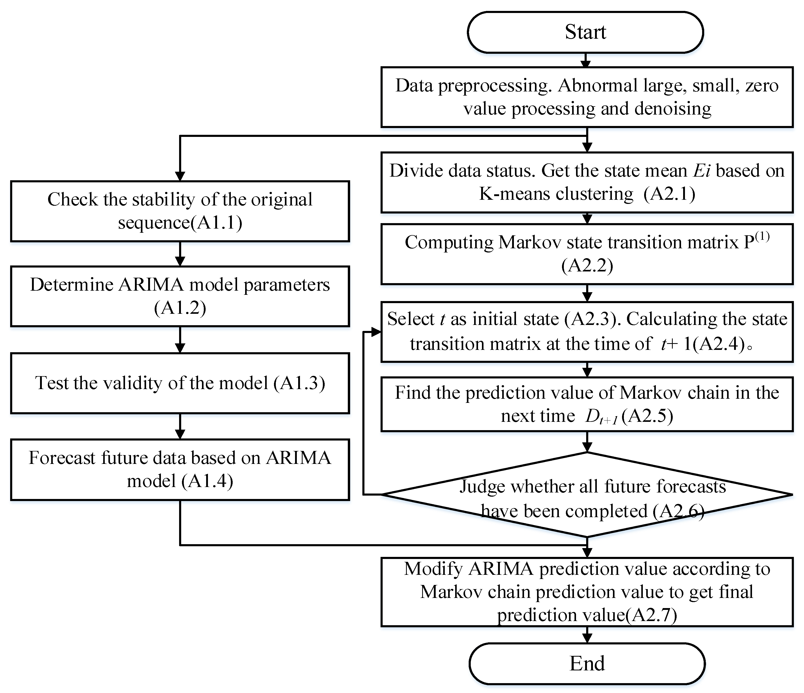
The daily water consumption prediction process based on the modified ARIMA prediction of Markov chain is demonstrated in Figure 1, and the specific process is presented as as Algorithm in

Table 2. Algorithm of data forecast based on the Markov chain-modified ARIMA model.

The Proposed Markov Chain-Modified ARIMA Prediction
A2.1	The water consumption data series $D_r$ is divided into N states. The k-means clustering algorithm is used to cluster the data sequence, and the states of each value in the sequences, the partition of N states, and the mean value Ei of state i are obtained.
A2.2	One step state transition matrix P(1) is calculated by Formula (4). According to the change of state in the sequence, the state transition frequency $f_{ij}$ is obtained, and then the transition probability $p_{ij}$ of each state is obtained according to Formula (5).
A2.3	Select the time t as the initial state, and get the initial state vector $X_t=\left(x_{t,1},x_{t,2},\cdots ,x_{t,N}\right)$. The data of the day before the forecast date is taken as the initial state.
A2.4	Calculate the state vector $X_{t+1}$ of water consumption to be predicted at the next time. Let $x_{t+1,i}$ represent the probability of state i at time t+1, then the state vector at time t+1 is the product of state vector at time t and transfer matrix, $X_{t+1}$= $X_t{P}^{\left(1\right)}$.
A2.5	The prediction value $D_{t+1}$ of future time based on Markov chain is calculated, which is expressed as Formula (6).
A2.6	Repeat steps A2.3–A2.6 to find the predicted water consumption of Markov chain at each time to be predicted.
A2.7	The prediction value of water consumption data at the time of t+n is obtained on the basis of the Markov chain prediction value and the ARIMA prediction value by Formula (7).

.

The algorithm flow is as follows in Figure 1.

4. Data Analysis

The effectiveness of the proposed algorithm is verified by examples. The daily water intake data of some water monitoring points in Guangdong Province from 2016 to 2017 were selected for the experiment. The daily water consumption data from January to December 2016 was used to build the model, and the data from January 2017 was used to test the validity of the model.

4.1. Data Pre-Processing

The abnormal values in the daily water consumption data, such as the noise, zero value, abnormally large values, or abnormally small values, may easily cause the error in the prediction model. Therefore, it is necessary to pre-process the data to remove the noise, abnormally large values, and other abnormalities. First, the abnormally large values of water consumption data were removed, on the basis of the pauta criterion, and the mean value was used to fill the abnormal values. For the noise data, the mode decomposition method was used to remove the high frequency data component as the noise.

Figure 2 and Figure 3 represent the original data and data after outlier processing of the two monitoring points, respectively. Figure 4 and Figure 5 demonstrate the outliers processed and de-noised data of two monitoring points, respectively.

4.2. Model Validation

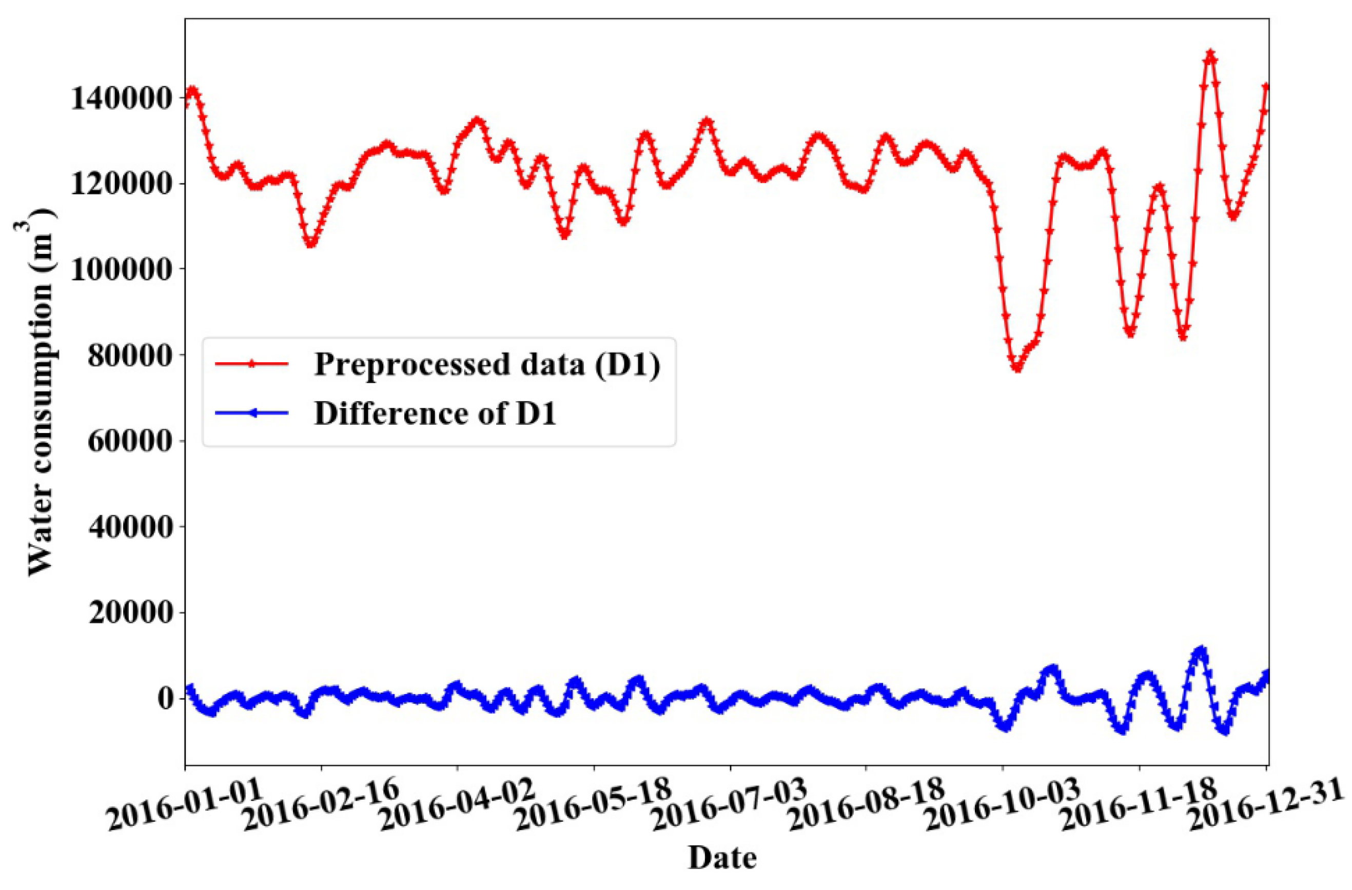
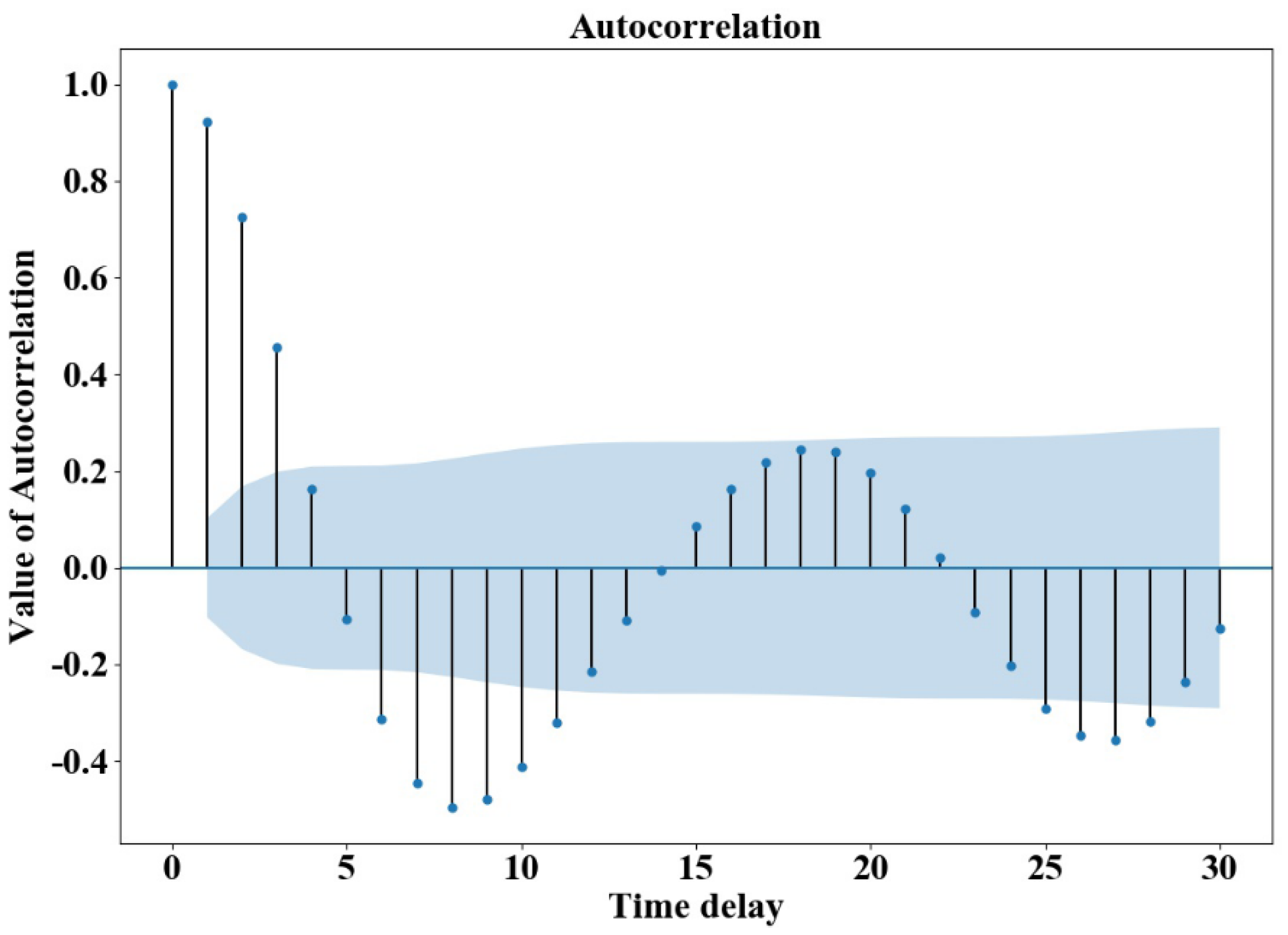
Firstly, the ARIMA analysis was performed on data 1 of the monitoring point. The water consumption data X₁ of the monitoring point 1 fluctuated within a wide range. To eliminate the fluctuation trend of its time series, the data sequence of X₁ was differentially processed and data sequence of DX₁ was obtained. As can be seen from Figure 6, the sequence after the first-order difference fluctuated steadily, around the mean value. Figure 7 displays the autocorrelation diagram after the first-order difference of the water consumption sequence. It can be seen from the figure that the autocorrelation coefficient is greater than zero for a long time, indicating the presence of a strong property between the sequences. The stationary state of the Augmented Dickey-Fuller (ADF) unit root test sequence was selected (see

Table 3. The unit root test results of the water consumption data difference at monitoring point 1.

ADF		Critical	Value	p-Value
test	1%	5%	10%
−6.99	−3.45	−2.87	−2.57	7.72 × 10−10

). The p-value of the unit root test was less than 0.05, suggesting the sequence after the first difference was a stationary sequence.

Further, it is necessary to judge whether there is correlation between the sequence data. If the sequence is white noise sequence, there is no information to be extracted, and the analysis of the sequence needs to be terminated. White noise test was conducted for the data after the first-order difference, and the results are shown in

Table 4. The white noise test results of the water consumption data difference at monitoring point 1.

Stat	5%
312.49	6.26 × 10−70

. The output p value is far less than 0.05, so the first-order difference sequence is a stationary non-white noise sequence.

The ARIMA model was fitted on the first-order stationary white noise sequence. The relative optimal model identification method was used to calculate the BIC information of all combinations of ARIMA (p, 1, q) at p and q less than or equal to 5. The model parameter with the minimum BIC information was selected and the BIC matrix bic_mat was as follows:

$$\left[\begin{array}{ccc}6808.99& 6334.83& \begin{array}{ccc}NaN& NaN& NaN\end{array}\\ 6092.91& NaN& \begin{array}{ccc}NaN& NaN& NaN\end{array}\\ \begin{array}{c}5376.16\\ 5247.25\\ 5214.20\end{array}& \begin{array}{c}5184.98\\ 5180.17\\ 5185.55\end{array}& \begin{array}{c}\begin{array}{ccc}5178.98& 5184.73& 5190.27\end{array}\\ \begin{array}{ccc}5184.70& \mathrm{NaN}& \mathrm{NaN}\end{array}\\ \begin{array}{ccc}NaN& 5189.91& 5193.39\end{array}\end{array}\end{array}\right]$$

(9)

When p value is 2 and q value is 2, the minimum BIC value is 5178.98. Then the sequence was fitted and analyzed with the model of ARIMA (2, 1, 2). The p-value of the white noise test around the residual was 0.93, which is white noise; therefore, the model is valid.

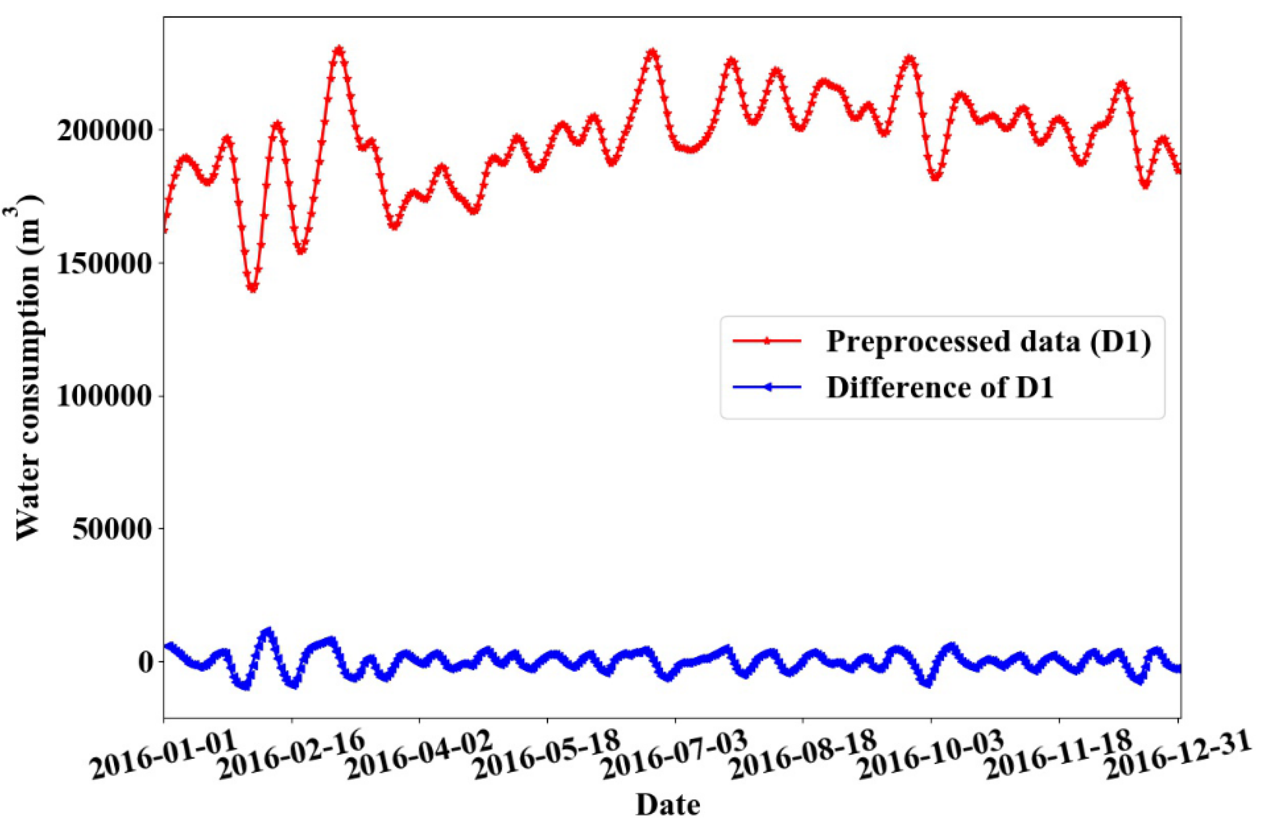
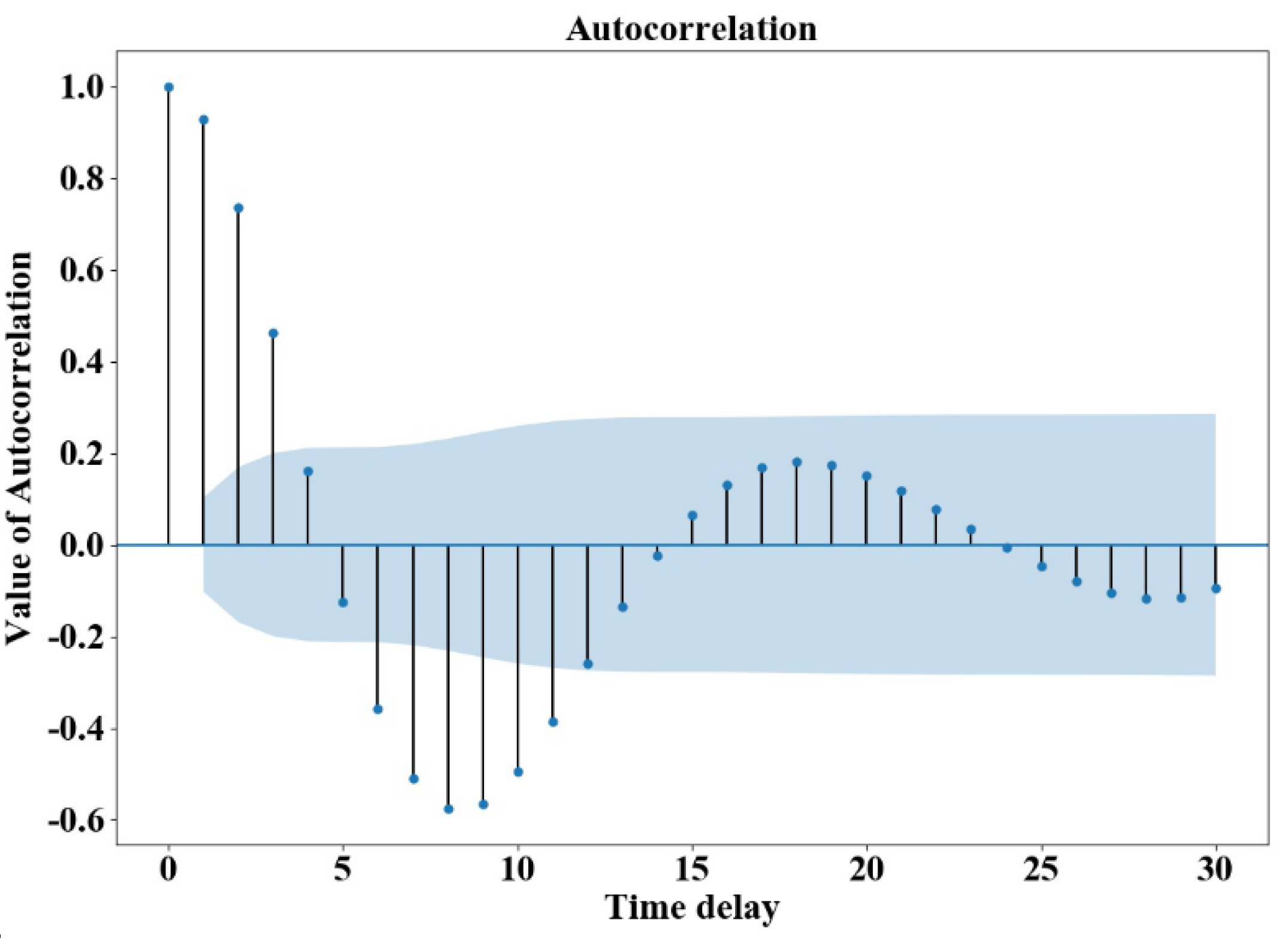
The same method was adopted to determine the water consumption data fitting model of monitoring point 2. The time sequence after the first-order difference of monitoring point 2 fluctuated stably around the mean value, as shown in Figure 8. And Figure 9 displays the autocorrelation diagram after the first-order difference of the water consumption sequence at monitoring point 2. The ADF unit root was selected to check the stable state of the sequence, and the results are shown in

Table 5. The unit root test results of water consumption data difference at monitoring point 2.

ADF		Critical Value		p-Value
test	1%	5%	10%
−8.18	−3.45	−2.87	−2.57	8.06 × 10−13

. The unit root test p-value was less than 0.05, which suggests the sequence after the first-order difference was a stationary sequence. The white noise test was carried out on the data after the first-order difference, and the results are shown in

Table 6. The white noise test results of water consumption data difference at monitoring point 2.

Stat	5%
316.44	8.62 × 10−71

. As it can be observed from the results, the output p-value was far less than 0.05; therefore, the sequence after the first-order difference was a stationary non-white noise sequence. It was determined that the ARIMA (p, 1, q) was less than or equal to 5 BIC information of all combinations. The p and q values, corresponding to the minimum BIC value, were all 2, and then the sequence was also fitted and analyzed with the model of ARIMA (2, 1, 2). The white noise test p-value of the residual was 0.90, which was white noise; thus, the model passed the test and is valid.

The longer the prediction period of the ARIMA model, the larger the prediction error, which causes error accumulation. Therefore, the proposed error correction method based on the Markov chain was used to correct the prediction results from the ARIMA model.

Firstly, on the basis of the Markov model, the training data were counted, and the state transition matrix and the one-step state transition value under each state were obtained. Subsequently, the future data prediction value was obtained as the future data trend. Then, the modified values were calculated on the basis of the prediction results of the Markov model.

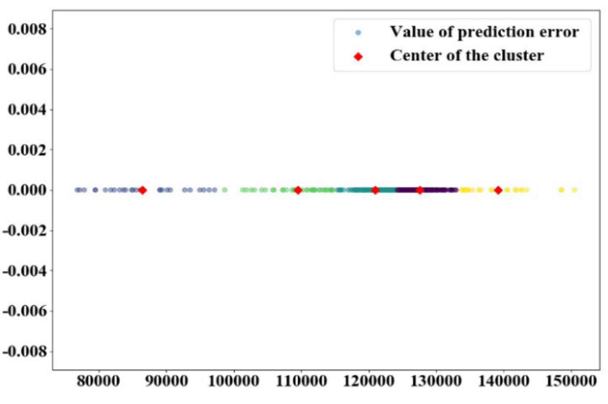
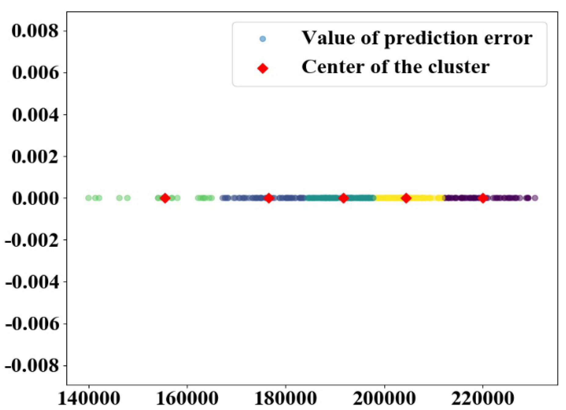
In the prediction based on the Markov chain, the state of data sequence was set to 5, and k-means algorithm was used to divide the state of data sequence. The cluster diagram of water consumption of monitoring point 1 and 2 are demonstrated in Figure 10 and Figure 11, respectively. The cluster center points of monitoring point 1 were the vector of [127561.19 86415.6 120963.62 109515.03 139121.21].

The Markov chain one-step state probability matrix of daily water consumption data at monitoring point 1 and point 2 are presented in the following equation, respectively, as follows:

$$\mathrm{p}=\left[\begin{array}{ccccc}0.87& 0& 0.11& 0& 0.02\\ 0& 0.89& 0& 0.11& 0\\ 0.09& 0& 0.86& 0.05& 0.01\\ 0& 0.08& 0.18& 0.75& 0\\ 0.18& 0& 0& 0& 0.82\end{array}\right]$$

(10)

$$\mathrm{p}=\left[\begin{array}{ccccc}0.85& 0& 0.77& 0.07& 0\\ 0& 0.81& 0& 0.13& 0.52\\ 0.08& 0.06& 0.85& 0& 0\\ 0.13& 0& 0& 0.87& 0\\ 0& 0.22& 0& 0& 0.78\end{array}\right]$$

(11)

Given the significance level $\alpha =$ 0.01, ${\chi }_{0.01}^2\left({\left(5-1\right)}^2\right)$ = 32 can be obtained by looking at the table. According to Equations (2) and (3), the statistical value ${\chi }^2$ of monitoring point 1 and 2 are 700.81 and 1268.14, respectively. Therefore, the Markov model can be used to predict the daily water consumption in future.

If the water consumption data of monitoring point 1 on that day is known, the state vector is set as P₀ = [0,0,0,0,1], according to the water consumption data, then the state vector of the next day is P₁ = $P_0\times P^{\left(1\right)}$. According to Equation (6), the predicted value is [127114.01 88890.54 121126.54 109786.08 137019.38]. In the same way, the prediction value of the next n days is calculated, accordingly, on the basis of the method of the modified ARIMA model, that is, combining the predicted value of the Markov chain to modify the predicted result of the ARIMA in proportion.

To test the prediction performance of the proposed model, the following prediction algorithms were compared and analyzed, which included the ARIMA prediction, the Markov prediction, and the modified ARIMA model (ARIMA-M).

In order to measure the stability and adaptability of the prediction model, root mean square error (RMSE) and coefficient of determination (R²), and the relative prediction error (RE) were selected as the evaluation indexes. The RMSE reflects the difference between the original value and the estimated value. The smaller the value, the closer the predicted value is to the real value, and the better the prediction effect. The R² can represent the whole fitting degree of the prediction model. The closer the R² is to 1, the better the fitting degree of the prediction value to the observation value, and the better the prediction performance of the model. The RE is the ratio of absolute error to the real value. The relative error reflects the reliability of the prediction. If the true real value and the predicted value of data r are T_i and Y_i, respectively, N is the number of predicted samples, and the average value of all data values is $\overline{T_i}$, then RMSE can be calculated through Equation (12), and R² and RE can be expressed by Equations (13) and (14).

$$RMSE=\sqrt{\frac{1}{N}{\displaystyle \sum }_{i=1}^N{\left(T_i-Y_i\right)}^2}$$

(12)

$$R^2=1-\frac{{{\displaystyle \sum }}_{i=1}^N{\left(T_i-Y_i\right)}^2}{{{\displaystyle \sum }}_{i=1}^N{\left(T_i-\overline{T_i}\right)}^2}$$

(13)

$$RE={\displaystyle \sum }_{i=1}^N\frac{\left(T_i-Y_i\right)}{T_i}\times \frac{1}{N}\times 100$$

(14)

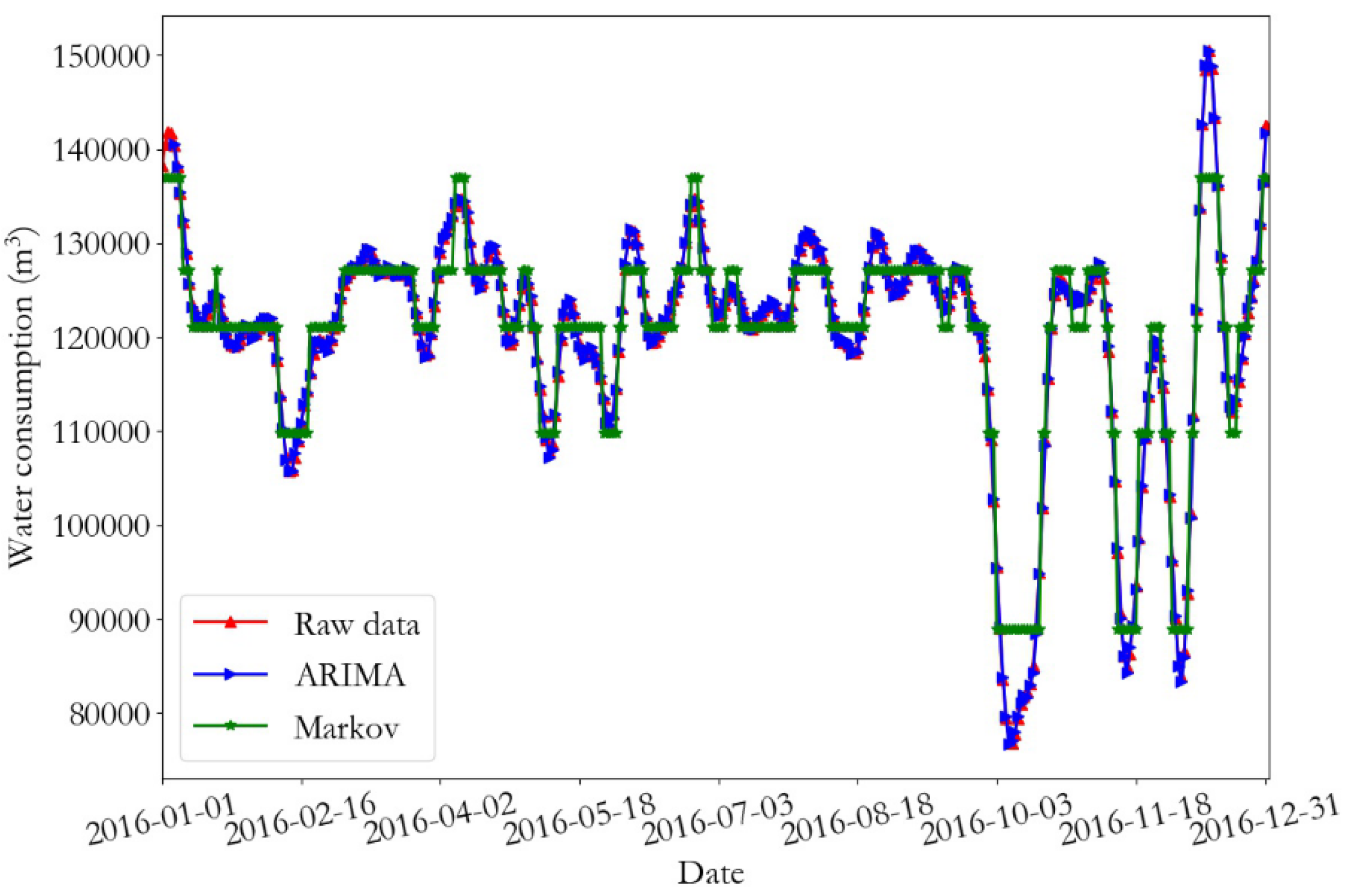
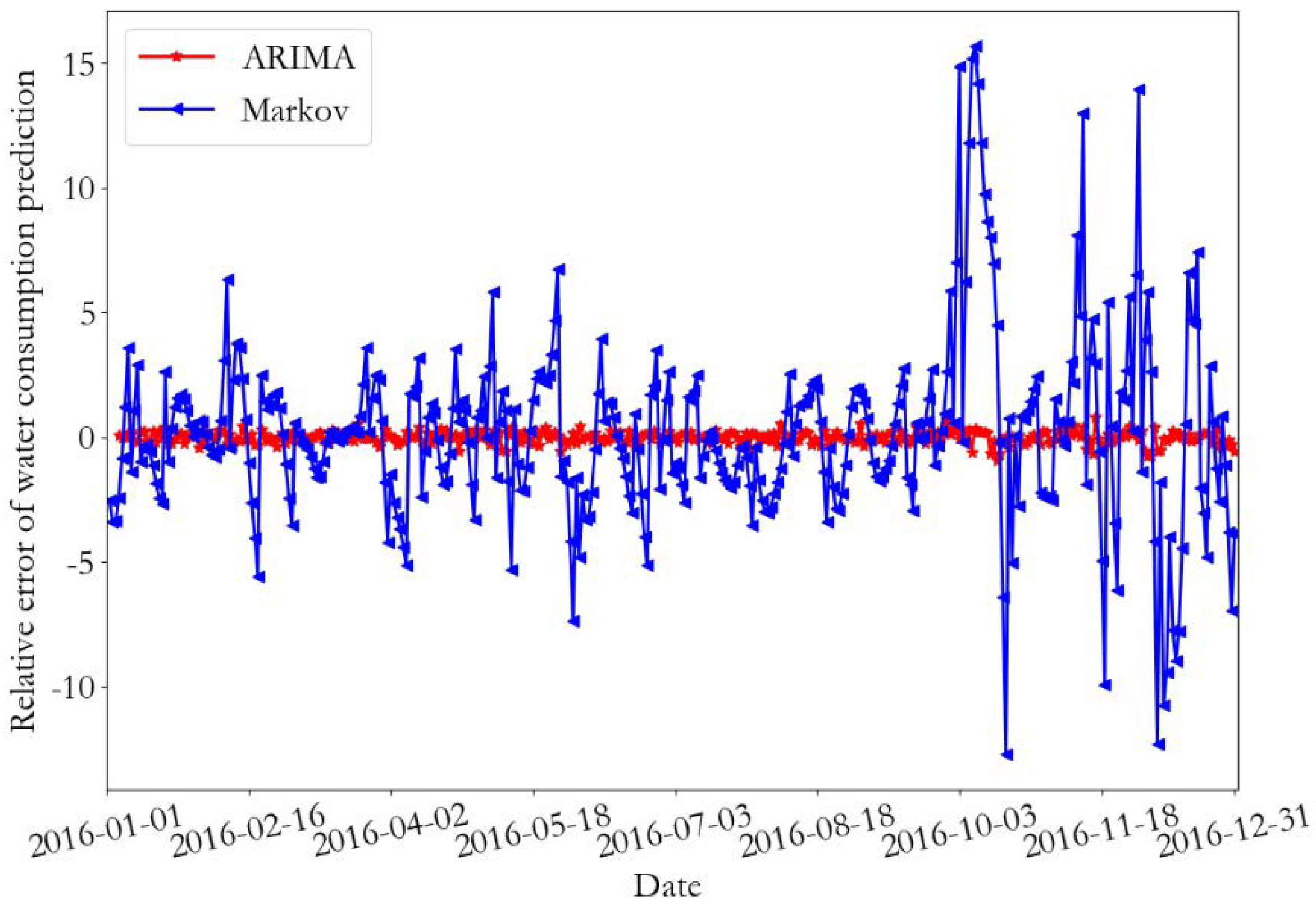
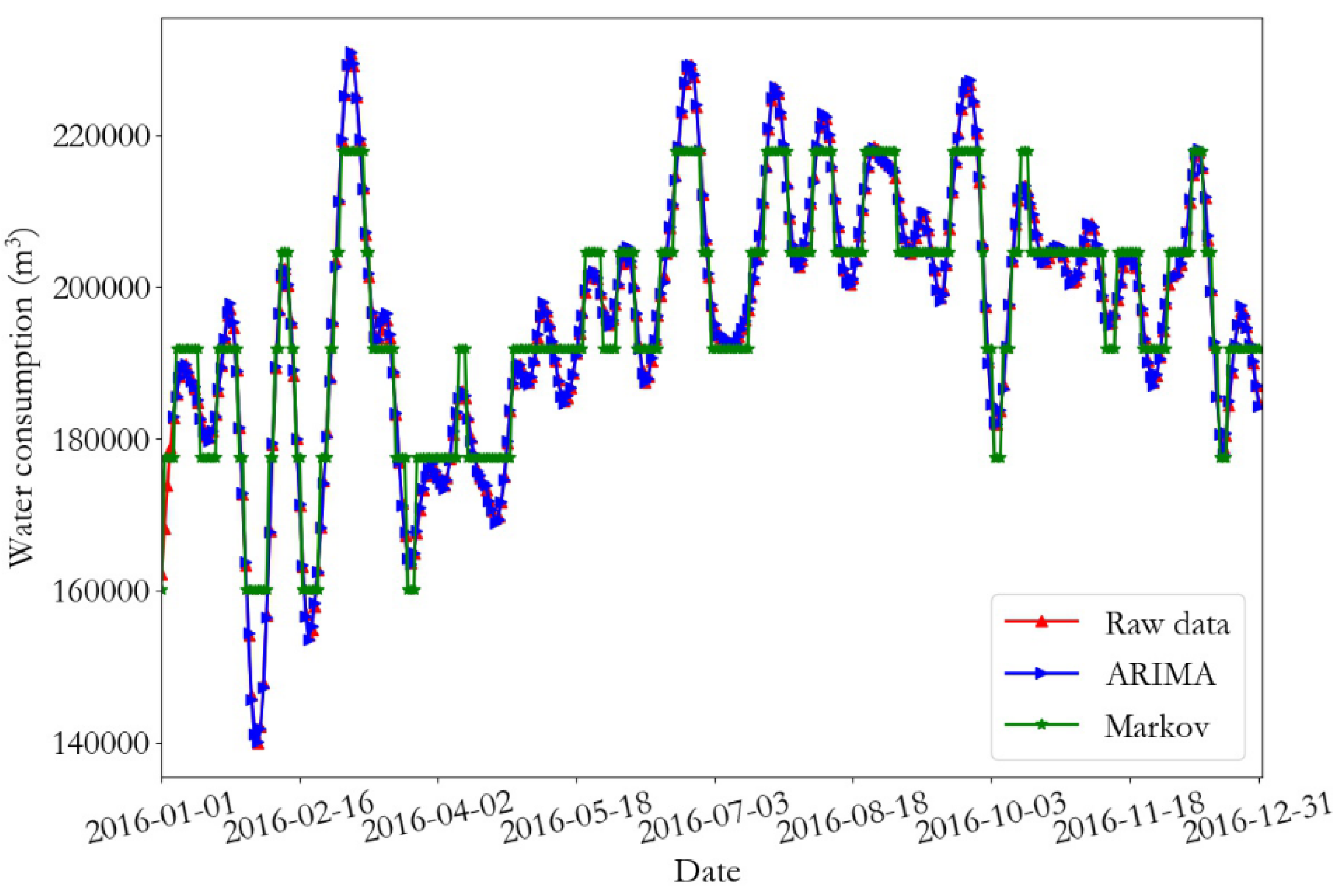
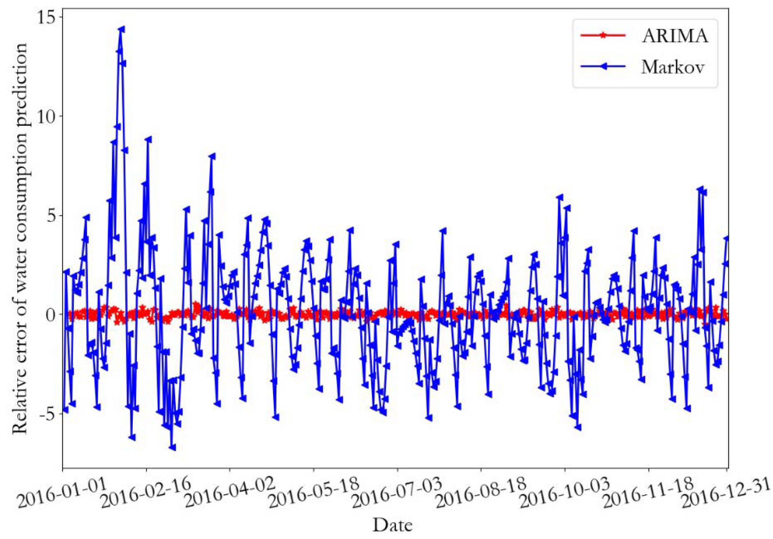
The prediction results and the relative error of the training data of monitoring point 1 are presented in Figure 12 and Figure 13, respectively. In addition, the prediction results and relative error curves of the training data of monitoring point 2 are demonstrated in Figure 14 and Figure 15, respectively. From the prediction results of the training data, it can be seen that the daily water consumption data of the two monitoring points predicted by the ARIMA were close to the real data value, and the overall trend predicted by the Markov was consistent with the predicted data; however, some errors were present. According to the error curve, it can be seen that the error of the ARIMA prediction was close to 0, and the error value of the Markov prediction at monitoring point 1 fluctuated between −12 and 15. Furthermore, the error value of the Markov prediction at monitoring point 2 fluctuated between −8 and 14.

Table 7. Prediction error of the training set at monitoring point 1.

	RMSE	R2	RE
ARIMA	275.17	0.9994	0.19
Markov	3919.08	0.90	2.47

and

Table 8. Prediction error of the training set at monitoring point 2.

	RMSE	R2	RE
ARIMA	300.93	0.9996	0.13
Markov	5628.25	0.89	2.34

show the prediction error of the ARIMA and the Markov model on the training dataset for monitoring point 1 and 2, respectively. According to the prediction data of monitoring point, the relative error (RE) of the ARIMA prediction was less than 0.2, and the coefficient of determination (R²) was close to 1; therefore, the training dataset can be better fitted by this model. The training data mean square error, coefficient of determination, and relative error rate of the Markov model were much larger than those of the ARIMA model. The relative errors of the Markov model for monitoring point 1 and monitoring point 2 were about 13 and 18 times that of the ARIMA, respectively. Therefore, the ARIMA model provided good fitting results for the training data, and the relative error RE of the Markov prediction was less than 2.5%, which can meet the requirements of the daily water consumption data prediction.

Therefore, the ARIMA and Markov combined data prediction model (ARIMA_M) can be used for the daily water consumption data prediction. The ARIMA model can fit the training data with high prediction accuracy. The Markov model can predict the trend of water consumption data on the basis of the training data of water consumption.

On the basis of the training set of daily water consumption, the ARIMA and Markov prediction models can be obtained by training. The ARIMA and the proposed ARIMA-M correction algorithm were used to predict the data of 20 days from 1 to 20 January 2017, in order to verify the validity of the model.

Table 9. Forecast value of monitoring point 1 during the following 10 days.

ID	Actual Water Consumption (m3)	ARIMA Forecast	ARIMA-M Forecast	RE of ARIMA Forecast (%)	RE of ARIMA-M Forecast (%)	RE Decrease of ARIMA-M Compared with ARIMA
1	136,226	157,671.60	131,251.64	15.74	−3.65	12.09
2	132,041.7	155,218.90	129,209.92	17.55	−2.14	15.41
3	130,589.9	153,773.05	128,006.34	17.75	−1.98	15.77
4	131,616.3	153,390.78	127,688.13	16.54	−2.98	13.56
5	134,733.5	153,969.18	128,169.61	14.28	−4.87	9.41
6	138,878.1	155,285.24	129,265.14	11.81	−6.92	4.89
7	142,930.4	157,046.25	130,731.08	9.88	−8.54	1.34
8	145,891.4	158,942.22	132,309.34	8.95	−9.31	−0.36
9	147,015.6	160,692.44	133,766.30	9.30	−9.01	0.29
10	146,597.7	162,080.79	134,922.01	10.56	−7.96	2.6

demonstrates the predicted values and errors of monitoring point 1 during the following 10 days. According to the future forecast data, the relative error RE of the ARIMA-M forecast can be reduced by 15.77%, compared to the ARIMA forecast.

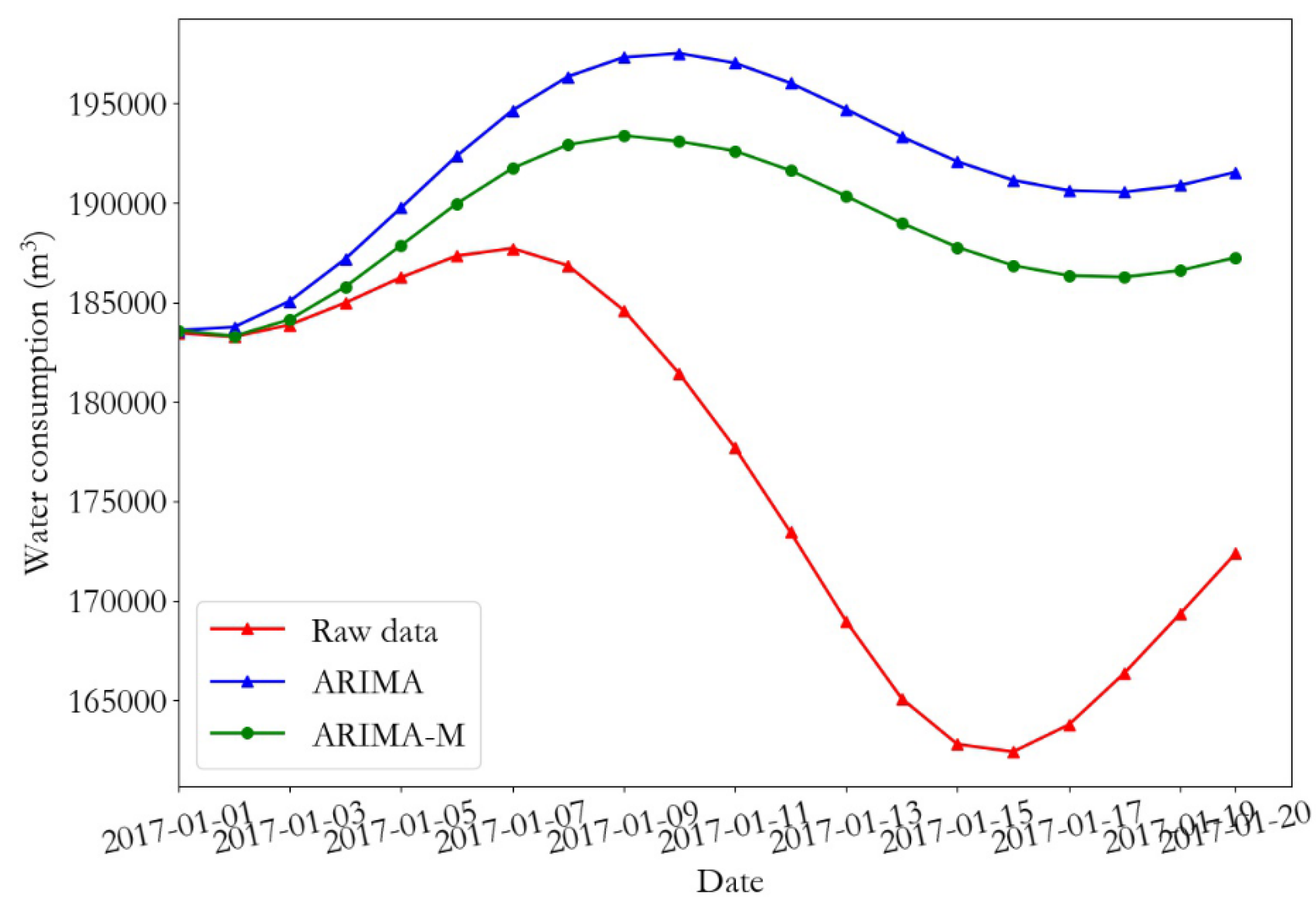
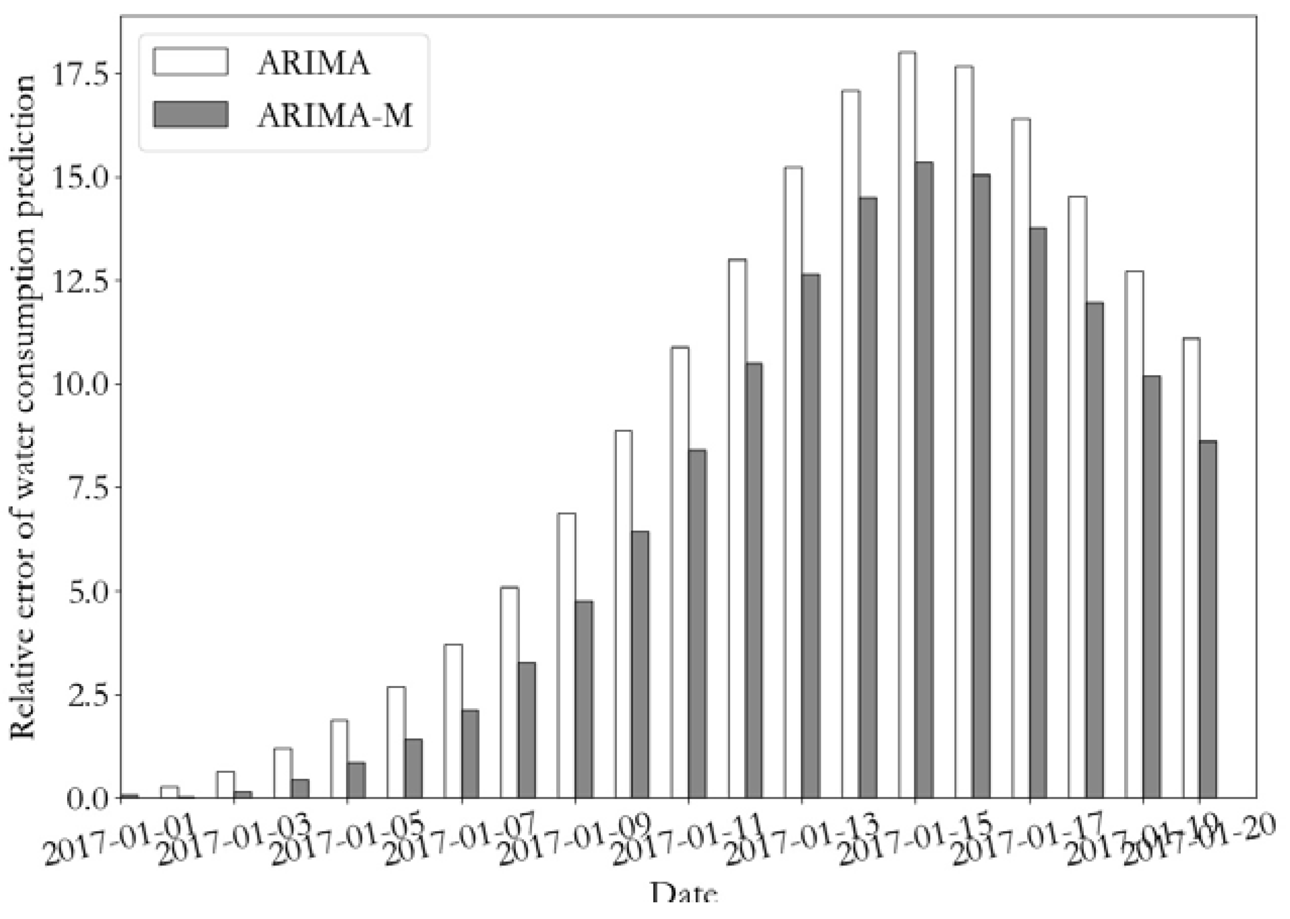
Figure 16 represents the total water consumption change and the relative error curve of monitoring point 2 for the following 20 days. Figure 17 shows the prediction error curve of water consumption of monitoring point 2 for the following 20 days using the ARIMA and ARIMA-M algorithms. It can be seen from the figure that the predicted value of the test data using the ARIMA-M model was closer to the real value, and that the prediction error was lower.

The prediction error of the ARIMA and the proposed ARIMA-M model in the overall test set of monitoring points 1 and 2 are presented in

Table 10. Prediction error of test set for monitoring point 1.

	RMSE	R2	RE
ARIMA	14,085.60	−0.04	8.07
ARIMA-M	10,569.32	0.42	6.10

and

Table 11. Prediction error of test set for monitoring point 2.

	RMSE	R2	RE
ARIMA	18,388.74	−3.04	8.07
ARIMA-M	15,003.34	−1.69	7.02

, respectively. It can be observed from the table that compared to the training data that the prediction error of the test data was greatly increased. At monitoring point 1, the RMSE reached to 14,085, the R² value was only −0.04, and the relative error reached 8.07. Using ARIMA-M, the RMSE of the predicted value of the test set was decreased by 25%, R² was increased by more than 10 times, and relative error was decreased by 24.4%, in comparison with the traditional ARIMA. For monitoring point 2, compared to the ARIMA, the RMSE of predicted value on ARIMA-M test set and the relative error were reduced by 18.4% and 13%, respectively.

According to the above analysis, the ARIMA model can provide a better fit for the changes of daily water consumption data of monitoring points, wheras the Markov can predict the trend of daily water consumption data within a certain error range. However, due to the randomness nature of the water consumption data, the prediction accuracy of the above model for the unknown data decreased, and the proposed ARIMA-M model can be used (1) to correct the deviation of the future daily water consumption prediction data, (2) to reduce the over fitting of the ARIMA model on the training data set, (3) to improve the prediction accuracy of the data, and (4) to provide data support for the decision makers, on the basis of daily water consumption data prediction value.

5. Discussion and Conclusions

Water resource is an important factor affecting the sustainable development of regional environment and society. Water consumption prediction can provide an important decision basis for regional water supply scheduling optimization. The accurate prediction and quota analysis of water consumption are helpful to the design of regional water use strategy, the improvement of emergency response ability of water resource management, and the improvement of water resource management and service level.

Therefore, a daily water consumption data prediction method is proposed in this study on the basis of the Markov model to modify the ARIMA prediction value. A complete set of schemes from actual data preprocessing to prediction analysis was provided. Firstly, the abnormal value of the data was corrected, and the data noise was effectively reduced by EEMD decomposition, and then further prediction and analysis were carried out. The main idea of the method was to get the data prediction model by fitting the historical data on the basis of the ARIMA model. Using the Markov model to predict the future trend of the data, the ARIMA model was modified, which corrected the great error caused by error superposition, and improved the accuracy of data prediction.

By analyzing the actual data of two water consumption monitoring points, the results showed that the prediction model of ARIMA and Markov had a small error for the training data; however, the prediction error to the unknown data in the future increased greatly. This meant that the model was overfitted. The ARIMA-M method can effectively improve the prediction accuracy of the future daily water consumption data for the monitoring point.

The main findings of this study include: (1) The prediction error of ARIMA model for unknown data can be corrected by using the data trend prediction results of the Markov model. (2) When the ARIMA model is used on a limited dataset, it can easily to produce over fitting. By the hybrid model based on ARIMA and Markov prediction model, the prediction error can be corrected and the prediction ability of the model can be improved. (3) The small predictive error on the training data does not mean that the prediction result of the model is good. Therefore, a hybrid model can be used to eliminate the effect of overfitting.

For future research, the seasonal characteristics of water consumption data can be analyzed, with the aim of further improvement in prediction accuracy. In addition, the adaptability of the model to the annual water consumption data, as well as the early warning of regional water security by integrating regional economic, social, and environmental data, are all worthy of further exploration.

References

- Yasar, A.; Bilgili, M.; Simsek, E. Water demand forecasting based on stepwise multiple nonlinear regression Analysis. Arab. J. Sci. Eng. 2012, 37, 2333–2341. [Google Scholar] [CrossRef]
- Brekke, L.; Larsen, M.D.; Ausburn, M.; Takaichi, L. Suburban water demand modeling using stepwise regression. J. AWWA 2002, 94, 65–75. [Google Scholar] [CrossRef]
- Brezonik, P.L.; Stadelmann, T.H. Analysis and predictive models of stormwater runoff volumes, loads, and pollutant concentrations from watersheds in the Twin Cities metropolitan area, Minnesota, USA. Water Res. 2002, 36, 1743–1757. [Google Scholar] [CrossRef]
- Adamowski, J.; Fung Chan, H.; Prasher, S.O.; Ozga-Zielinski, B.; Sliusarieva, A. Comparison of multiple linear and nonlinear regression, autoregressive integrated moving average, artificial neural network, and wavelet artificial neural network methods for urban water demand forecasting in Montreal, Canada. Water Resour. Res. 2012, 48. [Google Scholar] [CrossRef]
- Anderson, T.W.; Goodman, L.A. Statistical inference about markov chains. Ann. Math. Stat. 1957, 28, 89–110. [Google Scholar] [CrossRef]
- Tsaur, R.-C. A fuzzy time series-Markov chain model with an application to forecast the exchange rate between the Taiwan and US dollar. Int. J. Innov. Comput. Inf. Control 2012, 8, 4931–4942. [Google Scholar]
- Yu, G.; Hu, J.; Zhang, C.; Zhuang, L.; Song, J. Short-term traffic flow forecasting based on Markov chain model. In Proceedings of the IEEE IV2003 Intelligent Vehicles Symposium, Proceedings (Cat. No.03TH8683), Columbus, OH, USA, 9–11 June 2003; pp. 208–212. [Google Scholar]
- Carpinone, A.; Giorgio, M.; Langella, R.; Testa, A. Markov chain modeling for very-short-term wind power forecasting. Electr. Power Syst. Res. 2015, 122, 152–158. [Google Scholar] [CrossRef] [Green Version]
- Kani, S.A.P.; Ardehali, M.M. Very short-term wind speed prediction: A new artificial neural network–Markov chain model. Energy Convers. Manag. 2011, 52, 738–745. [Google Scholar] [CrossRef]
- Haan, C.T.; Allen, D.M.; Street, J.O. A markov chain model of daily rainfall. Water Resour. Res. 1976, 12, 443–449. [Google Scholar] [CrossRef]
- Su, F.; Wu, J.; He, S. Set pair analysis-Markov chain model for groundwater quality assessment and prediction: A case study of Xi’an city, China. Hum. Ecol. Risk Assess. Int. J. 2019, 25, 158–175. [Google Scholar] [CrossRef]
- Gagliardi, F.; Alvisi, S.; Kapelan, Z.; Franchini, M. A probabilistic short-term water demand forecasting model based on the markov chain. Water 2017, 9, 507. [Google Scholar] [CrossRef]
- Box, G. Box and jenkins: Time series analysis, forecasting and control. In A Very British Affair: Six Britons and the Development of Time Series Analysis During the 20th Century; Palgrave Macmillan: London, UK, 2013; pp. 161–215. ISBN 978-1-137-29126-4. [Google Scholar]
- Lippi, M.; Bertini, M.; Frasconi, P. Short-term traffic flow forecasting: An experimental comparison of time-series analysis and supervised learning. IEEE Trans. Intell. Transp. Syst. 2013, 14, 871–882. [Google Scholar] [CrossRef]
- Shvartser, L.; Shamir, U.; Feldman, M. Forecasting hourly water demands by pattern recognition approach. J. Water Resour. Plan. Manag. 1993, 119, 611–627. [Google Scholar] [CrossRef]
- Mombeni, H.A.; Rezaei, S.; Nadarajah, S.; Emami, M. Estimation of water demand in iran based on sarima models. Environ. Model. Assess. 2013, 18, 559–565. [Google Scholar] [CrossRef]
- Hao, C.-F.; Qiu, J.; Li, F.-F. Methodology for analyzing and predicting the runoff and sediment into a reservoir. Water 2017, 9, 440. [Google Scholar] [CrossRef] [Green Version]
- Graf, R. Distribution properties of a measurement series of river water temperature at different time resolution levels (based on the example of the lowland river noteć, Poland). Water 2018, 10, 203. [Google Scholar] [CrossRef] [Green Version]
- Wang, Z.Y.; Qiu, J.; Li, F.F. Hybrid models combining emd/eemd and arima for long-term streamflow forecasting. Water 2018, 10, 853. [Google Scholar] [CrossRef] [Green Version]
- Guarnaccia, C.; Tepedino, C.; Viccione, G.; Quartieri, J. Short-term forecasting of tank water levels serving urban water distribution networks with arima models. In Proceedings of the Frontiers in Water-Energy-Nexus—Nature-Based Solutions, Advanced Technologies and Best Practices for Environmental Sustainability, Cham, Switzerland, 19 September 2019; Naddeo, V., Balakrishnan, M., Choo, K.-H., Eds.; Springer: Cham, Switzerland, 2020; pp. 25–28. [Google Scholar]
- Donkor, E.A.; Mazzuchi, T.A.; Soyer, R.; Roberson, J.A. Urban water demand forecasting: Review of methods and models. J. Water Resour. Plan. Manag. 2014, 140, 146–159. [Google Scholar] [CrossRef]
- Bennett, C.; Stewart, R.A.; Beal, C.D. ANN-based residential water end-use demand forecasting model. Expert Syst. Appl. 2013, 40, 1014–1023. [Google Scholar] [CrossRef] [Green Version]
- Mouatadid, S.; Adamowski, J. Using extreme learning machines for short-term urban water demand forecasting. Urban Water J. 2017, 14, 630–638. [Google Scholar] [CrossRef]
- Adebiyi, A.A.; Adewumi, A.O.; Ayo, C.K. Comparison of arima and artificial neural networks models for stock price prediction. Environ. Model. Softw. 2002, 17, 219–228. [Google Scholar] [CrossRef] [Green Version]
- Sebri, M. Ann versus sarima models in forecasting residential water consumption in Tunisia. J. Water Sanit. Hyg. Dev. 2013, 3, 330–340. [Google Scholar] [CrossRef]
- Schittenkopf, C.; Deco, G.; Brauer, W. Two strategies to avoid overfitting in feedforward networks. Neural Netw. 1997, 10, 505–516. [Google Scholar] [CrossRef]
- Huang, N.E.; Shen, Z.; Long, S.R.; Wu, M.L.C.; Shih, H.H.; Zheng, Q.N.; Yen, N.C.; Tung, C.C.; Liu, H.H. The empirical mode decomposition and the Hilbert spectrum for nonlinear and non-stationary time series analysis. Proc. R. Soc. A Math. Phys. Eng. Sci. 1998, 454, 903–995. [Google Scholar] [CrossRef]
- Huang, N.E.; Wu, Z. A review on Hilbert-Huang transform: Method and its applications to geophysical studies. Rev. Geophys. 2008, 46. [Google Scholar] [CrossRef] [Green Version]
- Wu, Z.; Huang, N.E. A study of the characteristics of white noise using the empirical mode decomposition method. Proc. R. Soc. Lond. Ser. A Math. Phys. Eng. Sci. 2004, 460, 1597–1611. [Google Scholar] [CrossRef]
- Zhang, Y.; Kim, C.-W.; Tee, K.F. Maintenance management of offshore structures using Markov process model with random transition probabilities. Struct. Infrastruct. Eng. 2017, 13, 1068–1080. [Google Scholar] [CrossRef]
Figure 1.
Flow chart of water consumption forecast based on Markov chain correction.
Figure 2.
The original data and data after removing outliers of monitoring point 1.
Figure 3.
The original data and data after removing outliers of monitoring point 2.
Figure 4.
Data after removing outliers and after de-noising of the monitoring point 1.
Figure 5.
Data after removing outliers and after de-noising of the monitoring point 2.
Figure 6.
The original and first-order difference of total water consumption at the monitoring point 1.
Figure 7.
Autocorrelation chart of water consumption difference at the monitoring point 1.
Figure 8.
The original and first-order difference of total water consumption at monitoring point 2.
Figure 9.
Autocorrelation chart of water consumption difference at monitoring point 2.
Figure 10.
Data clustering of monitoring point 1.
Figure 11.
Data clustering of monitoring point 2.
Figure 12.
Prediction results from the training data at monitoring point 1.
Figure 13.
The relative error of the training data at monitoring point 1.
Figure 14.
Prediction results of the training data at monitoring point 2.
Figure 15.
The relative error of the training data at monitoring point 2.
Figure 16.
Prediction results of total water consumption at monitoring point 2.
Figure 17.
The relative error of total water consumption prediction at monitoring point 2.