Projections of Future Climate Change in the Vu Gia Thu Bon River Basin, Vietnam by Using Statistical DownScaling Model (SDSM)

Abstract

Future projections of anthropogenic climate change play a pivotal role in devising viable countermeasures to address climate-related risks. This study strove to construct future daily rainfall and maximum and minimum temperature scenarios in Vu Gia Thu Bon river basin by employing the Statistical DownScaling Model (SDSM). The model performance was evaluated by utilizing a Taylor diagram with dimensioned and dimensionless statistics. During validation, all model-performance measures show good ability in simulating extreme temperatures and reasonable ability for rainfall. Subsequently, a set of predictors derived from HadCM3 and CanESM2 was selected to generate ensembles of each climatic variables up to the end of 21st century. The generated outcomes exhibit a consistent increase in both extreme temperatures under all emission scenarios. The greatest changes in maximum and minimum temperature were predicted to increase by 2.67–3.9 °C and 1.24–1.96 °C between the 2080s and reference period for the worst-case scenarios. Conversely, there are several discrepancies in the projections of rainfall under different emission scenarios as well as among considered stations. The predicted outcomes indicate a significant decrease in rainfall by approximately 11.57%–17.68% at most stations by 2099. Moreover, all ensemble means were subjected to the overall and partial trend analysis by applying the Innovative-Şen trend analysis method. The results exhibit similar trend patterns, thereby indicating high stability and applicability of the SDSM. Generally, it is expected that these findings will contribute numerous valuable foundations to establish a framework for the assessment of climate change impacts at the river basin scale.

1. Introduction

There is high confidence that human activities are the main causes of the global warming of 1 °C [0.8–1.2 °C] above the pre-industrial levels, and this figure is likely to reach 1.5 °C between 2030 and 2052 [1]. As a consequence, natural and human systems have to deal with a wide range of climate-related risks. Based on a comparison between 1.5°C and 4°C warming, it is evident that the global average chance of major heatwave, agricultural drought, and 50-year return period river flood is likely to rise from 28%–92%, 24%–61%, 2.4%–5.4%, respectively [2]. Furthermore, Arnell et al. [3] utilized various indicators representing heat extremes, water resources, river and coastal flooding, droughts, agriculture, and energy use to estimate the potential impacts of climate change under different levels of climate forcings and socio-economic scenarios. With regard to climate extremes, Duan et al. [4] utilized the Database for Policy Decision-Making for Future Climate Change to explore possible changes in precipitation extremes based on six indices under 4 K warming climates compared to the Representative Concentration Pathway (RCP) 8.5 scenario of the Coupled Model Intercomparison Project phase 5 (CMIP5). Generally, this study indicated that precipitation extremes in China are likely to be more severe, and also highlighted the usefulness of employing large ensemble high-resolution climate simulations to address future uncertainties.

It is acknowledged that general circulation models (GCMs) are greatly supportive to the assessment of potential climate change impacts on multiple sectors at the global scale. Unfortunately, a horizontal resolution of GCMs is typically between 250 and 600 km, which cannot meet the requirements of most local impact studies. Additionally, an application of GCMs necessitates significant computational resources, thereby being unfeasible for most developing countries. Hence, many dynamical and statistical downscaling methods have arisen to overcome these key disadvantages of GCMs. Wilby and Wigley [5] presented a comprehensive review of the most commonly used downscaling techniques, discussing their limitations and challenges for future applications. Generally, statistical downscaling is more flexible, cheaper and less computationally demanding compared to dynamical downscaling [5,6].

Over the last few decades, there has been a proliferation of statistical downscaling tools for the sake of constructing future climate change scenarios at individual weather stations using various GCM outputs such as HadCM2, HadCM3, CGCM1, CGCM2, CGCM3, CanESM2, and IPSL-CM5A-MR. Khan et al. [7,8] quantified uncertainty in the performance of SDSM, Long Ashton Research Station Weather Generator (LARS-WG), and Artificial Neural Network (ANN) in downscaling daily precipitation and maximum and minimum temperatures at two meteorological stations in northern Quebec in Canada by comparing monthly means and variances, monthly mean dry and wet spell lengths, the cumulative frequency distributions of monthly mean of daily precipitation, and the distributions of monthly wet and dry days via many robust non-parametric statistical tests. Likewise, Etemadi et al. [9] compared the performance of SDSM and LARS-WG in terms of their uncertainty associated with temperature and precipitation projections in a vulnerable international wetland located in the Southwest Iran. Furthermore, Najafi and Kermani [10] proposed a new method based on fuzzy logic to investigate uncertainty associated with projected changes in temperature and precipitation using SDSM and Automated Statistical Downscaling (ASD) over the northern parts of Iran.

It is apparent that one of the most common themes of statistical downscaling application is to determine the superiority of statistical versus statistical, and/or statistical versus dynamical downscaling models. Particularly, two widely applied tools (i.e., SDSM and LARS-WG) were subjected to the well-conducted analysis by Hashmi et al. [11] and Hassan et al. [12] in the Clutha River (New Zealand) and Peninsular Malaysia respectively. Liu et al. [13] also compared the model performance of SDSM with the nonhomogeneous hidden Markov model in simulating daily precipitation over an arid basin in China, with annual precipitation mostly lower than 200 mm. Tryhorn and DeGaetano [14] compared SDSM and a bias-correction and spatial disaggregation technique, representing statistical downscaling approach, with the regional climate model HadRM3 representing dynamical approach in terms of their predictive ability in simulating extreme precipitation over the Northeastern United States. Lately, Campozano et al. [15] conducted a comparative study on the performance of SDSM and a number of artificial intelligence approaches such as ANNs and least squares support vector machines over the Paute River Basin in Southern Ecuador.

Another main aim of previous downscaling studies is to emphasize the importance of predictor selection methods, which should be employed carefully to deal with the most problematic aspect, called collinearity. Mahmood and Babel [16] proposed a quantitative procedure to eliminate the effect of multi-co-linearity in the selection of large–scale predictors. Particularly, the highest correlated predictor, called super predictor, is defined first. Then, the remaining highly correlated predictors are regressed individually in the presence of super predictor. Finally, a set of optimal predictors is obtained by considering the values of the percentage reduction in partial correlation with respect to the correlation coefficient [16,17]. This approach was also applied successfully by Hasan et al. [18], Iwadra et al. [19], and Shafiq et al. [20]. Lately, Yang et al. [21] presented a comparative study of the performance of three predictor selection methods such as correlation analysis (including Pearson’s and Spearman’s rank correlation coefficients), partial correlation analysis, and stepwise regression analysis in terms of the uncertainty assessment through a number of non-parametric statistical tests. The results revealed that stepwise regression analysis performs slightly better than its counterparts.

Apart from modeling conventional climatic variables (e.g., temperature and precipitation), the predictive abilities of statistical downscaling tools (e.g., SDSM) were also well documented for other exotic variables such as ground-level ozone and particulate matter [22], and reference evapotranspiration [23,24]. SDSM was also proved skillful in downscaling climate extremes and indices [17,25,26,27,28]. Additionally, SDSM was applied in combination with a hydrological model, namely Soil and Water Assessment Tool (SWAT), to characterize the responses of streamflow to future changes in precipitation, maximum and minimum temperatures over the upper Ishikari river basin, Japan [29]. Lately, Ahmadi et al. [30] integrated SDSM with the ANN and a rainfall–runoff model, called IHACRES, in order to investigate the impacts of climate change on surface runoff in the Kan watershed (Iran) under different representative concentration pathway scenarios derived from CanESM2. In general, it is highly evident that SDSM is such a fruitful tool for constructing future climate change scenarios.

In Vietnam, there have also been a number of salient case studies in the field of climate projections during the last few decades. Particularly, Ngo-Duc et al. [31] highlighted the advantage of utilizing the ensemble mean of three regional climate models (RCMs) in reproducing the climatological mean state and several extreme climate indices (i.e., TXx, TNn, and RX1day) over seven climate sub-regions of Vietnam. Likewise, Raghavan et al. [32] evaluated the downscaling ability of Providing REgional Climates for Impacts Studies (PRECIS) model in simulating mean state and extreme rainfall indices by using a subset of the Perturbed Physics Ensembles and their ensembles. It is discernible that most previous investigations employed dynamical downscaling approach by applying Conformal Cubic Atmospheric Model (CCAM), Regional Climate Model Version 3 (RegCM3), Regional Model (REMO), and PRECIS models. In the Vu Gia Thu Bon (VGTB) river basin, Thanh and Dutto [33], Nam et al. [34] employed a number of bias correction techniques to reduce systematic biases from the outputs of multiple GCMs/RCMs, which were subsequently used to assess the impacts of climate change on extreme flood events.

It is acknowledged that there are very few studies that make use of statistical downscaling tools (e.g., SDSM) to generate climate change scenarios over the Vu Gia Thu Bon river basin as well as Vietnam. It is worth noting that most hydrological and hydraulic modeling tools, e.g., SWAT, IHACRES, Precipitation Runoff Modeling System (PRMS), Integrated Catchment Water Modelling (CATCHMOD), Hydrologic Engineering Centers River Analysis System (HEC-RAS), MIKE, etc., necessitate historical and future climate data as primary inputs for assessing the impacts of climate change on water resources at the river basin scale. Hence, there is an urgent need for the construction of future daily climate data at individual meteorological stations by applying statistical downscaling approach. In an attempt to cover this lacuna, the present study was conducted by employing SDSM for the sake of constructing future climate scenarios over the Vu Gia Thu Bon river basin under multiple emission scenarios based on the outputs of two commonly used GCMs (i.e., HadCM3 and CanESM2). On the whole, this study will be conducive to the climate-related risk reduction and adaptation in the study area.

2. Materials and Methods

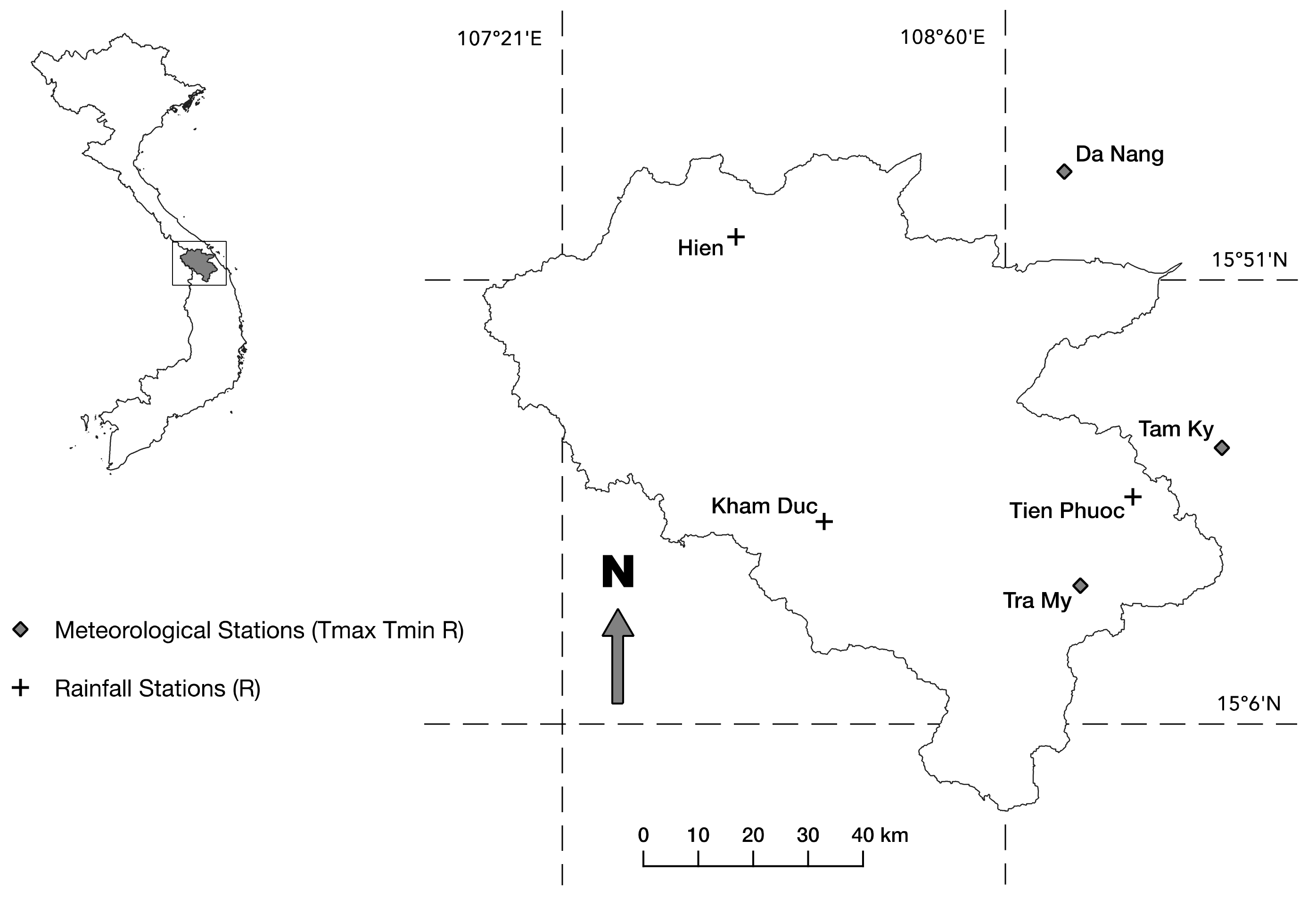
2.1. Study Area and Data

The Vu Gia Thu Bon river basin, located in the Central Vietnam (Figure 1), is one of the largest internal drainage systems of Vietnam. Geographically, this river basin lies approximately between 14°95′ – 16°06′ N in latitude and 107°21′—108°46′ E in longitude, and has a total area of around 10,350 km². Administratively, most area of the VGTB river basin is situated in Quang Nam province and Da Nang city, and a very small proportion (nearly 3%) is located in Kon Tum province. The VGTB river basin consists of two main rivers, namely Vu Gia and Thu Bon, originating in the Ngoc Linh Mountain and flowing toward the sea at Cua Dai estuary. The general climate of the VGTB river basin is classified into the tropical monsoon climate (Am) according to the updated world map of the Köppen–Geiger climate classification [35]. Based on the well–known global climate datasets (WorldClim 2) developed by Fick and Hijmans [36], the average temperature ranges from 19.3–25.3 °C for the present period (1970–2000). The total amount of annual rainfall varies from 1900–3000 mm, mainly contributed by rainfall during the rainy season lasting from May to November. It is acknowledged that the VGTB river basin is greatly crucial to the livelihood of local residents with regard to water, food, energy, cultural and recreational activities [37]. However, the recurrence of floods during the rainy season and droughts as well as water shortages during the dry season poses many serious challenges to local decision-makers [37,38]. Therefore, future projections of climate variables will provide various insights into the integrated water resources management in the VGTB river basin.

The observed daily rainfall (R), maximum (Tmax) and minimum (Tmin) temperature datasets at three meteorological stations and three rainfall stations as shown in Figure 1 were provided by the Mid-Central Regional Hydro-Meteorological Centre for the period 1979–2010. Additionally, the National Centre for Environmental Prediction (NCEP) reanalysis dataset [39] were obtained for the purpose of model calibration and validation. Likewise, two sets of 26 large-scale predictors derived from HadCM3 (A2 and B2) and CanESM2 (RCP2.6, 4.5 and 8.5) were selected for the sake of scenario generation for the 2020s (2010–39), 2050s (2040–69), and 2080s (2070–99).

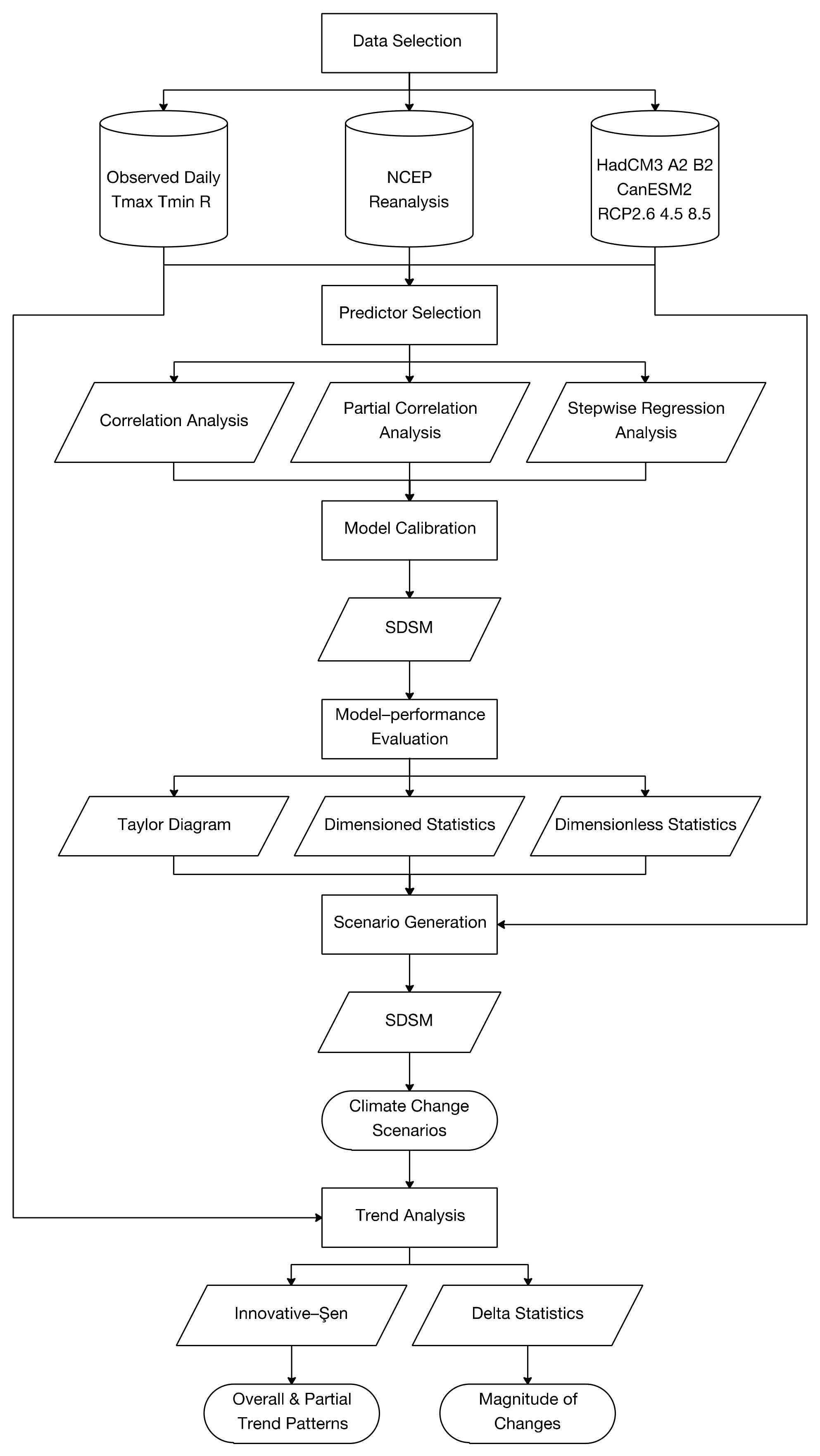
2.2. Research Framework

Figure 2 depicts a brief description of the methodology employed in this study. The first step is to select input data including observed daily rainfall, maximum and minimum temperatures which are predictand variables, and a set of predictors derived from NCEP reanalysis dataset and from two GCM outputs. In SDSM, the functions of quality control and data transformation allow users to inspect the integrity of input data and unexpected errors (e.g., missing data, suspect values or wrong encoding), and to transform data in case variables of interest are not normally distributed.

After obtaining complete datasets, the preliminary task is to define a set of candidate predictors for each climatic variable at individual stations. In essence, the fundamental principle of all statistical downscaling approaches is to determine empirical–statistical relationships between large-scale predictors with local predictands. It is widely acknowledged that potential predictors should have high abilities in describing atmospheric circulation, thickness, stability, and moisture content [40]. Additionally, the potential predictors should be well modeled by GCMs and available to be retrieved from multiple sources of GCMs [6,40]. In general, selecting appropriate predictors constitutes a great proportion of successful models. In the present study, the choice of appropriate predictors is carried out by applying correlation analysis, partial correlation analysis and stepwise regression analysis in order to avoid the collinearity issue and remain a set of predictors with strongly and consistently correlated with the considered predictands. The applicability of these aforementioned methods was documented in detail by Yang et al. [21].

The further step is to reproduce ensembles of daily series for the present period based on well–calibrated models, which are then subjected to the model-performance evaluation by applying the well-known Taylor diagram and a number of dimensioned and dimensionless statistics. Subsequently, generation of future climate is executed by using selected predictors derived from GCM outputs. Finally, trend analysis is performed to identify overall and partial trend patterns by constructing the Innovative-Şen trend plots, and to determine the magnitude of changes between the future periods and reference period by calculating delta statistics. It is worth mentioning that the model calibration and scenario generation for the present and future periods are performed by executing respective functions in SDSM. The following sections describe briefly the fundamental basis of SDSM, model-performance measures and the innovative-Şen trend analysis method.

2.3. The Statistical DownScaling Model

The Statistical DownScaling Model was introduced by Wilby et al. [40] as a freely available tool to support decision making processes with regard to climate change impact assessment at local scale. According to an exhaustive review after ten years of the first version in 2001 by Wilby and Dawson [41] and many case studies as described above, it is documented that SDSM can be used for reproducing present climate, predicting future climate based on multiple scenarios, infilling and hindcasting missing data. SDSM is applicable to not only conventional climatic variables (e.g., temperature and precipitation), but also exotic variables (e.g., air quality or reference evapotranspiration) and climate extremes. SDSM is also used in combination with other tools (e.g., hydrological and hydraulic models) to develop an integrated framework for uncertainty assessment.

SDSM is established based on a combination of the stochastic weather generator and regression-based methods [40,42]. Having selected appropriate predictors, SDSM is calibrated by either dual simplex or ordinary least squares. It is documented that dual simplex should be applied to remove the effect of instability of regression coefficients for nonorthogonal predictors [27,43], while ordinary least squares method is faster [42]. It is also necessary to specify a number of model structures during calibration stage. Particularly, unconditional process, in which a direct link is assumed between predictors and predictand, is selected for temperature, while conditional process, which assumes the presence of an intermediate process between predictors and predictand, is selected for rainfall. It is also advisable that data transformation should be implemented in case the predictand variables (e.g., rainfall) are not normally distributed. In this study, a fourth root transformation was employed. Additionally, SDSM provides calibrated parameters for three types of sub-periods such as monthly, seasonal, and annual models. The present study selected monthly option, which calculates different model parameters for each month. Having established a set of well-calibrated model parameters, SDSM reproduces ensembles of present climate data using predictors derived from NCEP reanalysis dataset for the sake of model-performance evaluation, and generates ensembles of future climate data using predictors derived from HadCM3 and CanESM2. Wilby and Dawson [42] expounded the theory of SDSM as well as exemplified a very clear step-by-step procedure to perform SDSM.

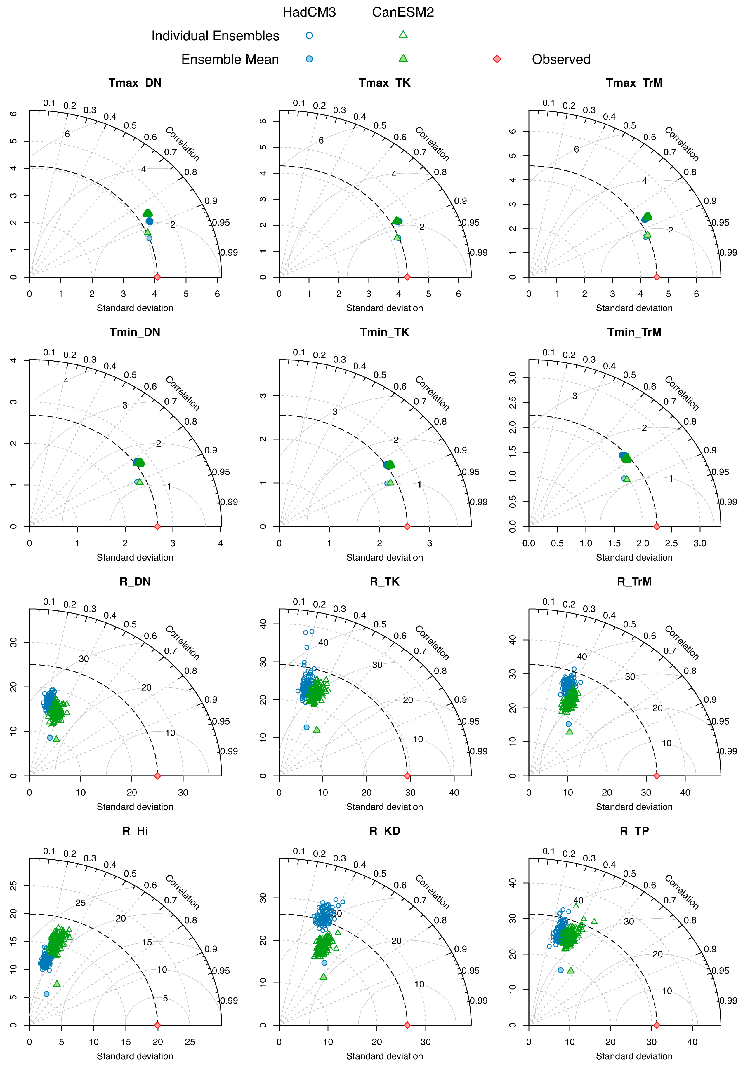
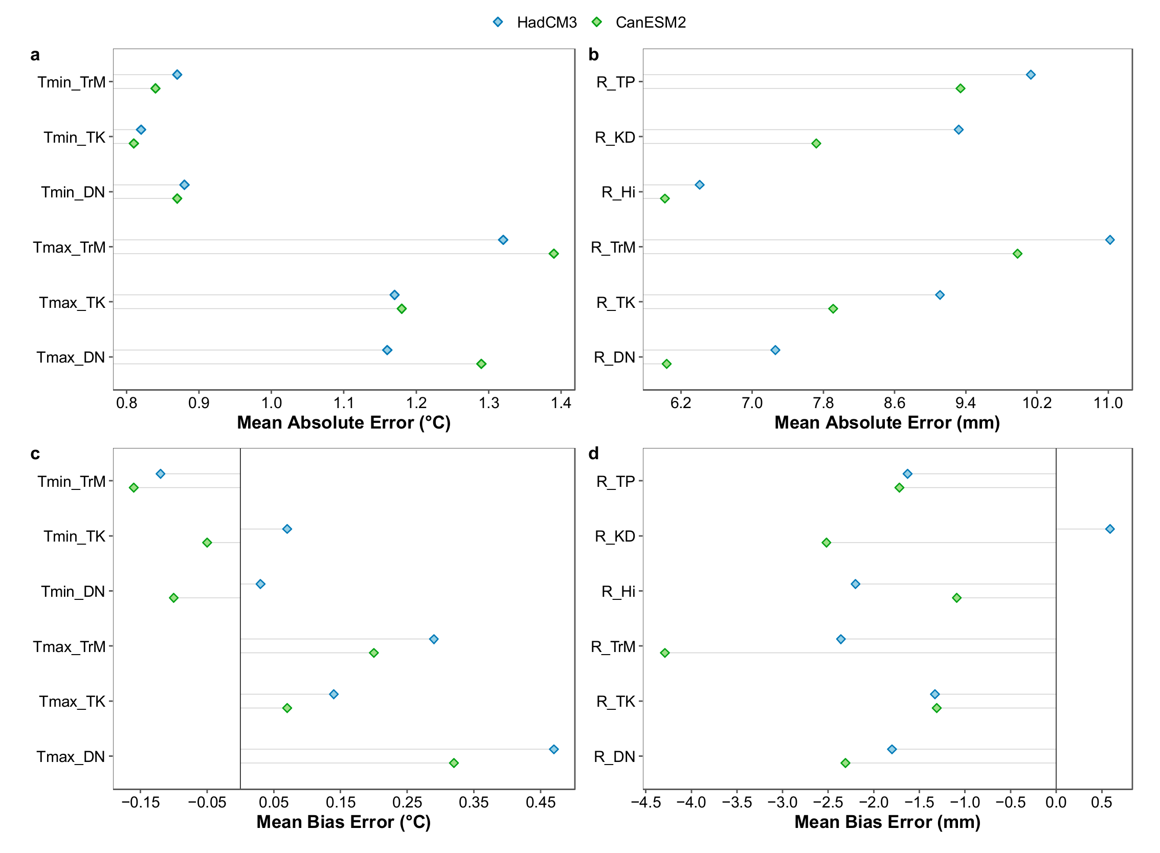
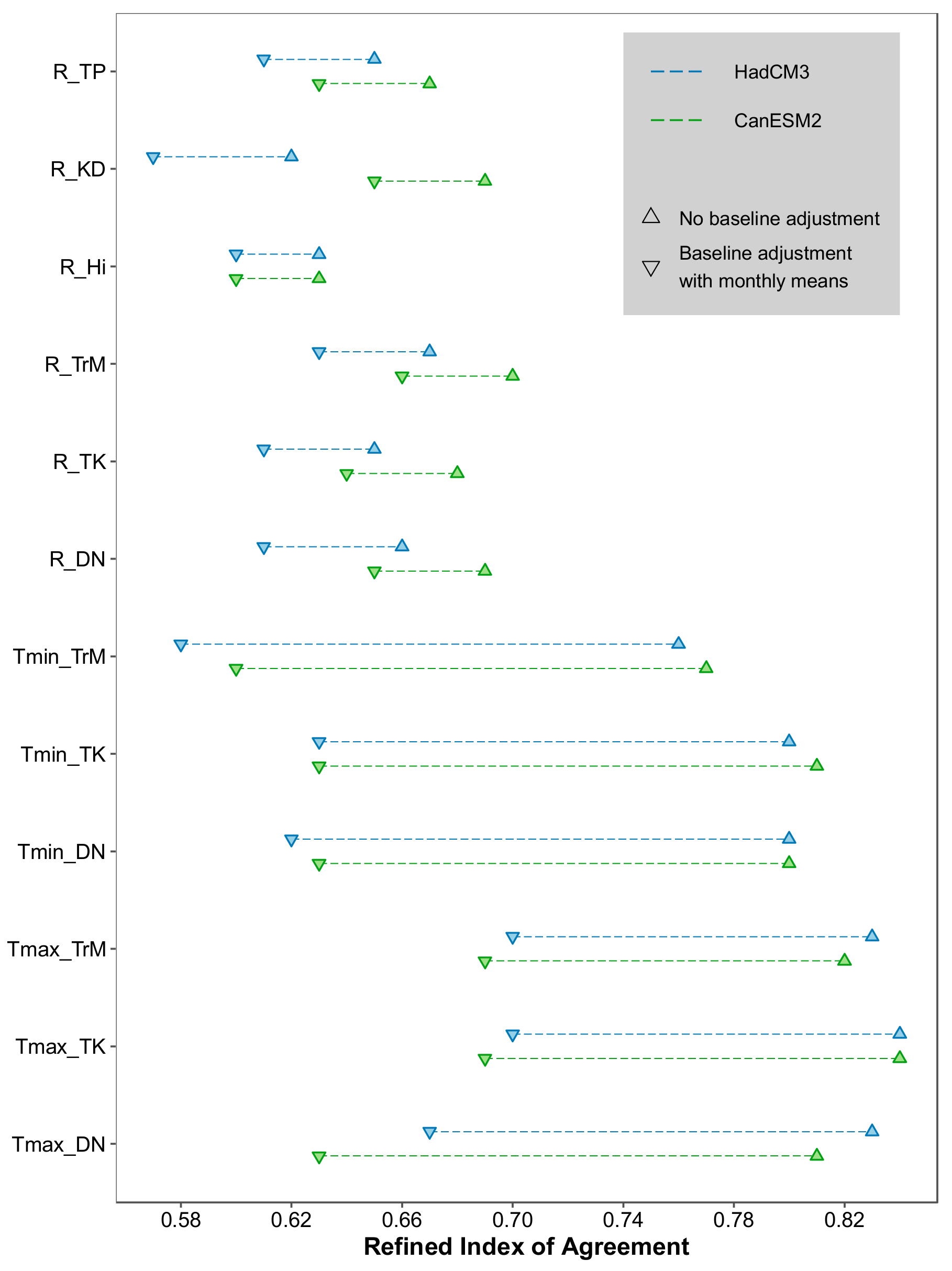
2.4. Evaluation of Model Performance

There is a widespread agreement that a reasonable model should exhibit high correlation, low errors and similar variations compared to the observations. The Taylor diagram, devised by Taylor [44], is a powerful tool to measure these aspects graphically via correlation coefficient, root-mean-square difference and standard deviations of the test field (i.e., models) and reference field (i.e., observations). Therefore, this study applied the Taylor diagram to compare individual ensemble members with the ensemble mean during validation.

It is substantiated that the correlation–based and sum-of-squares-based measures are greatly sensitive to the presence of extreme values and/or outliers, thereby suggesting that these measures are not appropriate and should not be utilized to address model performance [45,46,47,48]. It is also advisable to employ the absolute-error/deviation-based measures. Hence, the present study applied mean absolute error (MAE) and mean bias error (MBE), representing dimensioned statistics, and a refined index of agreement with/without baseline adjustments, representing dimensionless statistics.

MAE is used to quantify average model-prediction error in the units of analyzed variables. The lower values of MAE indicate better prediction. MBE gives an indication of average model bias, which can be over-prediction or under-prediction in case the values of MBE are positive or negative. In addition, a refined index of agreement (d_r), introduced by Willmott et al. [49], is employed to measure the predictive ability of SDSM models. The values of d_r are bounded by −1 and +1. Generally, a positive value of d_r indicates a good model. Legates and McCabe [50] further explained that the performance of a model is better than the baseline value (e.g., observed mean) when d_r > 0.5. It is also recommended to adjust baseline values [46,49,50,51] when evaluating model performance for variables of interest, which exhibit high seasonal variations. Hence, monthly means are used in combination with the overall values when calculating the refined index of agreement.

$$MAE=\frac{1}{n}{\displaystyle \sum }_{i=1}^n\left|P_i-O_i\right|$$

(1)

$$MBE=\frac{1}{n}{\displaystyle \sum }_{i=1}^n\left(P_i-O_i\right)$$

(2)

$$d_r=\left\{\begin{array}{c}\begin{array}{c}1-\frac{{{\displaystyle \sum }}_{i=1}^n\left|P_i-O_i\right|}{c{{\displaystyle \sum }}_{i=1}^n\left|O_i-\overline{O}\right|},\mathit{when}\\ {\displaystyle {\displaystyle \sum }_{i=1}^n}\left|P_i-O_i\right|\le c{\displaystyle {\displaystyle \sum }_{i=1}^n}\left|O_i-\overline{O}\right|\end{array}\\ \begin{array}{c}\frac{c{{\displaystyle \sum }}_{i=1}^n\left|O_i-\overline{O}\right|}{{{\displaystyle \sum }}_{i=1}^n\left|P_i-O_i\right|}-1,\mathit{when}\\ {\displaystyle {\displaystyle \sum }_{i=1}^n}\left|P_i-O_i\right|>c{\displaystyle {\displaystyle \sum }_{i=1}^n}\left|O_i-\overline{O}\right|\end{array}\end{array}\right.$$

(3)

where n is the length of the data series. P_i and O_i stand for the predicted and observed values of daily rainfall and maximum and minimum temperatures, respectively. The overbars are used to indicate overall means for the whole analyzed period. c is a scaling coefficient and is preferably set to be 2 [49,51]. In case of calculating an index of agreement with baseline adjustments ($d_r^{\prime }$), the observed overall mean ($\overline{O}$) is replaced by the monthly mean ($\overline{O^{\prime }}$).

2.5. The Innovative-Şen Trend Analysis Method

The innovative-Şen trend analysis (ITA) method, originated by Şen [52], is applied to identify overall and partial trends in a given hydro–meteorological time series. In comparison with a number of classical trend analysis methods (including parametric and nonparametric statistical trend tests), the ITA method has an advantage of not considering any restrictive assumptions such as normal distribution, serial independence and length of data. As a matter of fact, this study was clearly inspired by a well–conducted investigation, which analyzed multi-duration trend possibilities in the global monthly temperature records [53]. In the present study, the ITA method was employed to examine trend behavior of Tmax, Tmin, and rainfall time series between the reference period (1980–2009) and the future periods (2010–39, 2040–69, and 2070–99) based on multiple scenarios. Specifically, the innovative-Şen trend plot is constructed by plotting the sorted series for the reference period on the x-axis against the sorted series for the future periods on the y-axis. The next step is to draw the 1:1 (45°) straight line and ±10% error lines on the Cartesian coordinate system. Theoretically, the 45° straight line divides the innovative-Şen trend plot into two equal regions. The upper/lower triangular areas indicate increasing/decreasing trends, while 45° straight line corresponds to trend-free cases. Additionally, it is evident that trend slope is stronger in case the scatter points fall far away from the 45° straight line [52].

3. Results and Discussion

3.1. Model Calibration and Validation

The observed daily rainfall, Tmax and Tmin datasets and appropriate predictors derived from NCEP reanalysis dataset were used to calibrate and validate SDSM models for the period 1979–1990 and 1991–2001, respectively. SDSM can generate up to a maximum of 100 ensemble members. Figure 3 presents the Taylor diagrams used as means of comparing each ensemble member with respective ensemble mean for Tmax, Tmin, and rainfall at individual stations during validation procedure. Based on the relative position of all points on such diagrams, it is discernible that SDSM produces similar outputs between all considered stations for each of climatic variables in the study area. In particular, all ensemble means show higher correlation and lower error compared to each ensemble member. With regard to the variations of downscaled results, the ensemble means of Tmax at all meteorological stations capture the observed standard deviations better than each ensemble member and all solid points lie approximately on the black dashed arc, implying that the amplitude of variations downscaled by SDSM for Tmax are similar to the observed ones. Conversely, the variations of ensemble mean of Tmin and rainfall are lower than each ensemble member as well as the observed values. It is also apparent that the downscaled outputs show a greater degree of variability in rainfall compared to Tmax and Tmin, which could be attributable to the conditional process during calibration procedure. In general, this study only used the values of ensemble means for further calculation for the sake of simplicity.

In addition to the graphical approach, it is strongly recommended to report both dimensioned and dimensionless measures for the purpose of model-performance evaluation [46,51]. Figure 4 and Figure 5 depict the validation results for HadCM3 and CanESM2 models by applying the MAE, MBE, and refined index of agreement with/without baseline adjustments respectively. As shown in Figure 4, the values of MAE vary approximately from 0.81–0.88 °C, 1.16–1.39 °C, and 6–11 mm for Tmin, Tmax, and rainfall respectively. It is visible that the model errors in Tmax are significantly greater than Tmin. In comparison, HadCM3 and CanESM2 models produce fairly similar error in modeling daily Tmax and Tmin, while HadCM3 model generates consistently higher error in simulating daily rainfall compared to CanESM2 model. Moreover, daily rainfall is mainly underestimated during validation, with MBE values around −1.1 to −4.3 mm. Conversely, daily Tmax is consistently overestimated at all meteorological stations, with the values of MBE ranging 0.07–0.47 °C. In the case of daily Tmin, there is a slight discrepancy in the validated outputs by using HadCM3 and CanESM2 models at Da Nang and Tam Ky stations, while daily Tmin at Tra My station is underestimated, with the MBE values around −0.12 to −0.16 °C. In general, the validation results show that the magnitude of these dimensioned statistics is within acceptable range on the daily time scale.

Furthermore, Figure 5 shows additional validation results by applying dimensionless statistics. According to the refined index of agreement without baseline adjustment (d_r), it is apparent that the performance of SDSM is more skillful in downscaling daily Tmax and Tmin (d_r = 0.76–0.84) compared to daily rainfall (d_r = 0.62–0.70). These values are fairly similar and slightly higher than the figures found by Najafi and Kermani [10] for the case Tmax, Tmin, and rainfall, respectively. In addition, the values of refined index of agreement with baseline adjustments by monthly means ($d_r^{\prime }$) range approximately from 0.57–0.70, which are significantly lower than the respective d_r values. According to the values of d_r and $d_r^{\prime }$, HadCM3 and CanESM2 models show similar skill in simulating Tmax and Tmin, while CanESM2 model performs better than HadCM3 for the case of rainfall at most stations. On the whole, all calculated values of d_r and $d_r^{\prime }$ reveal that the magnitude of average model error, represented by MAE, is lower than the average reference error, represented by 2 × mean absolute deviation, thereby suggesting that the calibrated model parameters can be reasonably used for future scenario generation.

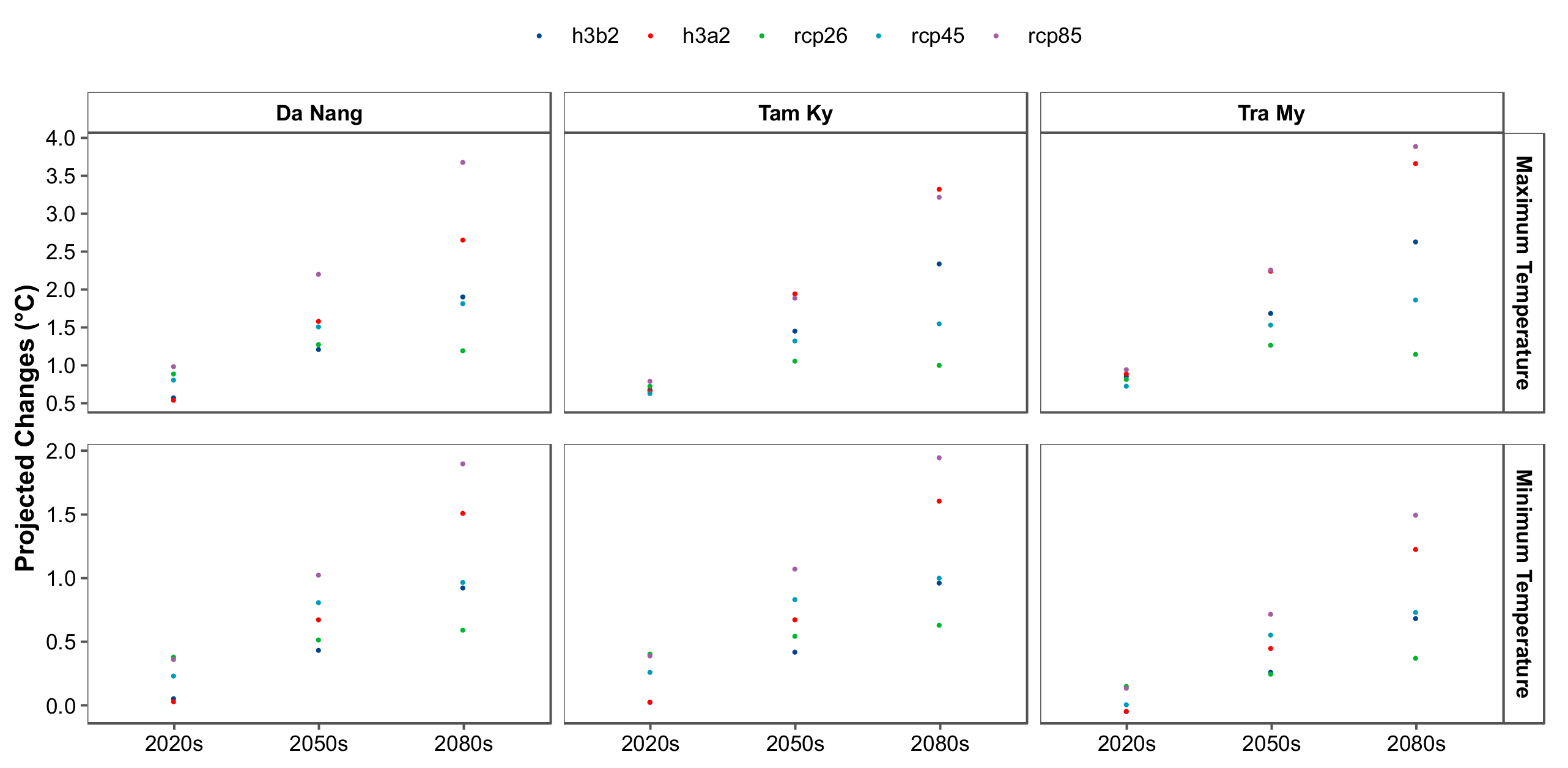
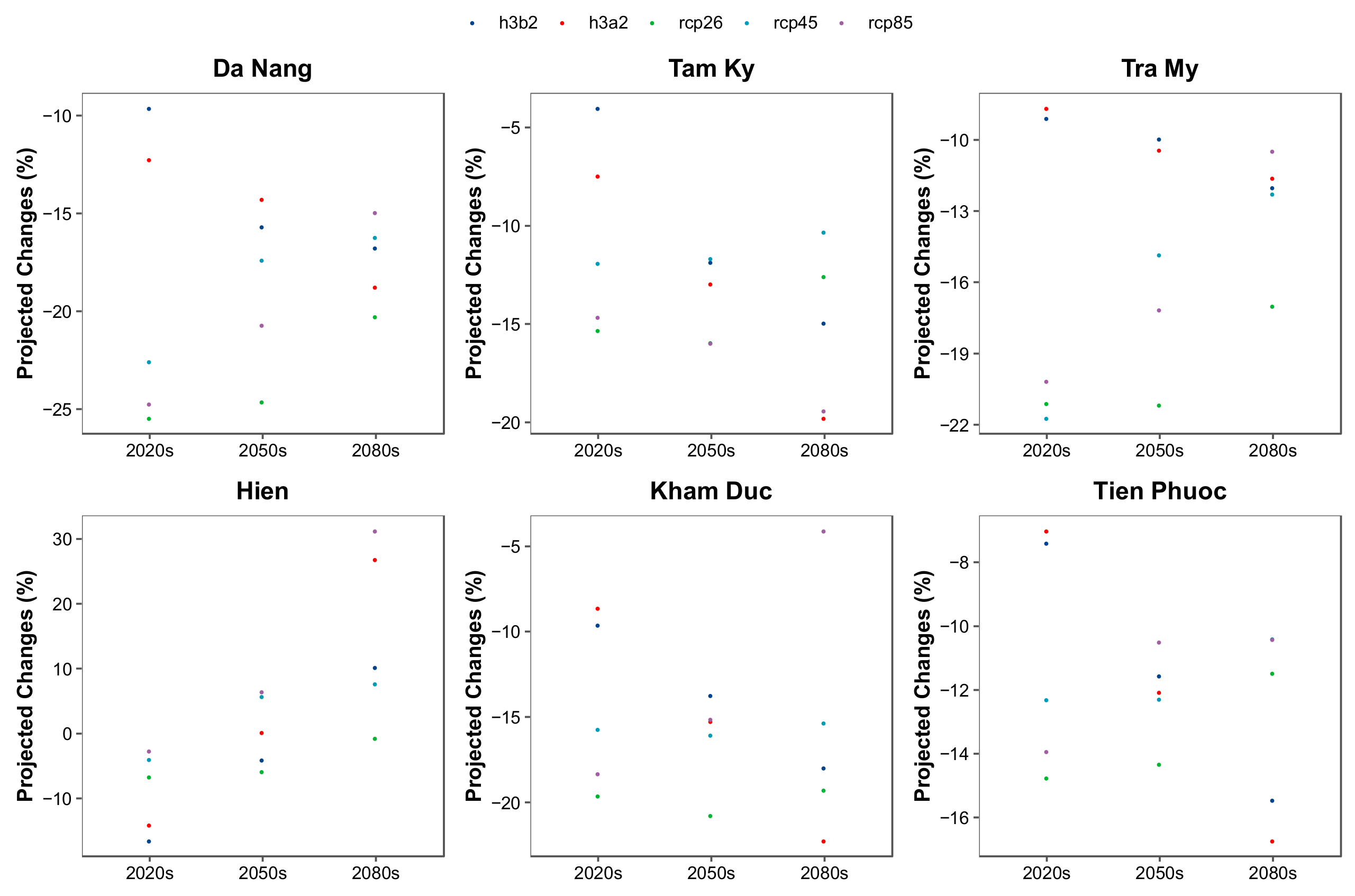
3.2. Future Climate Projections

Figure 6 and Figure 7 present projected changes in annual average Tmax, Tmin, and average annual rainfall by calculating delta statistics (absolute and percentage difference for the case Tmax, Tmin, and rainfall respectively) between the 2020s, 2050s, 2080s, and the reference period under multiple scenarios such as HadCM3 A2 B2 and CanESM2 RCP2.6, 4.5, 8.5. As shown in Figure 6, there is a profound warming tendency in the VGTB river basin, and Tmax is projected to experience a greater degree of warming compared to Tmin at all meteorological stations. Additionally, there is a minor difference between all considered scenarios during the 2020s, while the middle and far-future periods exhibit larger variations in the degrees of warming. Particularly, Tmax and Tmin are predicted to increase by 0.55–1.0 °C and are lower than 0.41 °C, respectively, during the 2020s compared to the reference period. In the middle-future period (2050s), the figures are likely to increase by 1.07–2.27 °C and 0.26–1.08 °C for the case Tmax and Tmin, respectively. During the 2080s, the worst-case scenarios (i.e., HadCM3 A2 and CanESM2 RCP8.5) are responsible for the greatest increase in Tmax and Tmin by 2.67–3.90 °C and 1.24–1.96 °C, which are significantly higher than the figures for the remaining scenarios varying approximately from 1.01–2.65 °C and 0.38–1.01 °C, respectively. In comparison, these findings, to some extent, are in agreement with those found by Ngo-Duc et al. [31], in which the 2 m temperature was projected to increase significantly in most parts of Vietnam for the near and middle-future periods by utilizing ensembles of three RCMs.

In contrast to Tmax and Tmin, there are a number of discrepancies in the future projections of annual rainfall between considered stations under all scenarios. Figure 7 shows that annual rainfall is predicted to decrease significantly at most stations over the VGTB river basin. Out of six stations, five stations reveal that HadCM3 model exhibits a greater decrease when considering from near- to far-future periods, while CanESM2 model shows an opposite tendency on the whole. A detailed description of projected changes in annual rainfall can be obtained from Figure 7. During the far-future period (2080s), the average annual rainfall is likely to decrease by 14.9%–20.3%, 10.3%–19.8%, 10.5%–17.0%, 4.1%–22.2%, and 10.3%–19.8% compared to the reference period at Da Nang, Tam Ky, Tra My, Kham Duc, and Tien Phuoc stations respectively. Conversely, annual rainfall at Hien station is projected to increase significantly between the 2080s and reference period, even though it is mainly dominated by decreasing trends for the near- and middle-future periods. Particularly, the greatest increasing trends in annual rainfall at Hien station are estimated by 26.9%–31.3% for the 2080s under the worst-case scenarios (HadCM3 A2 and CanESM2 RCP8.5). It is worth noting that several previous studies [33,34] indicated increasing trends in annual rainfall over the VGTB river basin by applying bias correction approaches, which differs from those found in the present study. To a certain extent, these findings reflect various uncertainties in future projections of daily rainfall. Generally, uncertainties in climate projections are mainly attributable to internal climate variability, downscaling methods and tools, and input data used (including observed predictand variables and GCM-derived predictors). This study utilized a set of predictors derived from HadCM3 and CanESM2 models, representing manifold emission scenarios. It is also advisable to apply other downscaling methods (e.g., bias correction, LARS-WG, ASD or artificial intelligence approaches) along with SDSM [9]. Another suggestion is to use more than one set of potential predictors for each climate variable at individual stations to obtain possible range of climate variation in the future periods.

In addition to calculating delta statistics for the purpose of trend analysis, the present study also pertains to the overall and partial trend identification between the 2020s, 2050s, 2080s, and the reference period under multiple scenarios. As shown in Figure 8, the innovative-Şen trend plots for Tmax and Tmin also indicate a consistent warming trend over the VGTB river basin. It is apparent that all of plus and filled circle points, representing the 2050s and 2080s periods, are located in the upper-triangular areas implying significantly upward trends, while most of filled diamond points, representing the 2020s, fall alongside the 1:1 (45°) straight lines and within ±10% error lines revealing insignificant rises. In line with the results of delta statistics, it is also evident that the largest deviations from the 1:1 line can be found for the worst-case scenarios (i.e., HadCM3 A2 and CanESM2 RCP8.5) for the 2080s, which indicates the greatest trend slope compared to the remaining scenarios. With regard to partial trend assessment, Tmax and Tmin exhibit the same sub-trend patterns. Particularly, most of these sub-trends are likely to be more significant when the corresponding values get higher, thereby suggesting an evident indication of the occurrence of hot weather events in the future periods.

Concerning annual rainfall trend analysis in the VGTB river basin, it is discernible that decreasing trends are detected significantly at most stations for the future periods. Da Nang and Tra My stations show fairly similar sub-trends patterns, and the high value sub-groups are characterized by significant decreases irrespective of considered future scenarios. In the case of Tam Ky and Kham Duc stations, the largest deviations from the 1:1 (45°) straight lines can be found in the medium value sub-groups, which implies the greatest declines under all scenarios. As for rainfall trend assessment at Tien Phuoc station, most of scatter points fall alongside the lower error line revealing marginal decreases. As expected, rainfall trend behaviors at Hien station differ clearly from the other stations. Particularly, the worst-case scenarios (i.e., HadCM3 A2 and CanESM2 RCP8.5) for the 2080s show significant increases irrespective of low-, medium-, and high-value sub-groups, while the remaining scenarios exhibit almost trend–free behavior. It is worth mentioning that ensembles of synthetic Tmax and Tmin series produced by SDSM mostly comply with the linear form, since the large majority of scatter points are located in the straight data lines. Meanwhile, ensembles of synthetic rainfall series generated by SDSM can be non-monotonic form. There is also high similarity in the sub-trend patterns of most considered climatic variables under all scenarios, implying high stability and applicability of SDSM.

4. Conclusions

A complete and appropriate historical and future climate dataset is a prerequisite for a successful study of climate change impacts on a given sector. Accordingly, the main aim of this study was to construct daily rainfall, maximum and minimum temperatures for the near-, middle-, and far-future periods over the VGTB river basin by employing SDSM tool and a set of GCM-derived predictors retrieved from HadCM3 (A2 and B2) and CanESM2 (RCP2.6, 4.5, and 8.5). Additionally, the evaluation of model performance was carried out by a combination of the Taylor diagrams, dimensioned and dimensionless statistics. During validation, all model-performance measures are within permissible ranges indicating that calibrated model parameters can be reasonably used for scenario generation. It is also noting that SDSM shows greater predictive ability in modeling daily maximum and minimum temperatures compared to daily rainfall as suggested by comparing the refined index of agreement with/without baseline adjustments.

The results of trend analysis of future climatic changes by calculating delta statistics are in accordance with those found by the ITA method. Particularly, the VGTB river basin is expected to experience a consistent warming tendency, with a greater degree of warming for the case Tmax compared to Tmin at all stations. During the far-future period (2070–99), the worst-case scenarios (i.e., HadCM3 A2 and CanESM2) were predicted to increase by 2.67–3.90 °C and 1.24–1.96 °C for the case Tmax and Tmin, respectively, which are significantly higher than the figures for the remaining scenarios as suggested by comparing delta statistics as well as examining the relative position of scatter points in the innovative-Şen trend plots. With regard to daily rainfall, the downscaled outputs show greater degree of variability compared to Tmax and Tmin. Moreover, the future projections of annual rainfall are mostly dominated by decreasing trends, with the magnitude varying approximately 11.57%–17.68% at most stations during the 2080s. In general, these outcomes imply that the VGTB river basin is likely to be hotter and drier in the future periods, which may cause potential issues relating to agricultural activities and water consumption. It is expected that these findings will be informative and supportive to further investigations and practical adaptation strategies in the context of climate emergency.

References

1. IPCC. 2018: Global Warming of 1.5 °C; An IPCC Special Report on the impacts of global warming of 1.5°C above pre-industrial levels and related global greenhouse gas emission pathways, in the context of strengthening the global response to the threat of climate change, sustainable development, and efforts to eradicate poverty; Masson-Delmotte, V.P., Zhai, H.-O., Pörtner, D., Roberts, J., Skea, P.R., Shukla, A., Pirani, W., Moufouma-Okia, C., Péan, R., Pidcock, S., Eds.; IPCC: Geneva, Switzerland, 2018; In Press. [Google Scholar]
2. Arnell, N.W.; Lowe, J.A.; Challinor, A.; Osborn, T. Global and regional impacts of climate change at different levels of global temperature increase. Clim. Chang. 2019, 155, 377–391. [Google Scholar] [CrossRef] [Green Version]
3. Arnell, N.W.; Lowe, J.A.; Bernie, D.; Nicholls, R.J.; Brown, S.; Challinor, A.J.; Osborn, T.J. The global and regional impacts of climate change under representative concentration pathway forcings and shared socioeconomic pathway socioeconomic scenarios. Environ. Res. Lett. 2019, 14, 084046. [Google Scholar] [CrossRef]
4. Duan, W.; Hanasaki, N.; Shiogama, H.; Chen, Y.; Zou, S.; Nover, D.; Zhou, B.; Wang, Y. Evaluation and Future Projection of Chinese Precipitation Extremes Using Large Ensemble High-Resolution Climate Simulations. J. Clim. 2019, 32, 2169–2183. [Google Scholar] [CrossRef]
5. Wilby, R.L.; Wigley, T. Downscaling general circulation model output: A review of methods and limitations. Prog. Phys. Geog. 1997, 21, 530–548. [Google Scholar] [CrossRef]
6. Benestad, R. Empirical-statistical downscaling in climate modeling. Eos. Trans. Am. Geophys. Union. 2004, 85, 417–422. [Google Scholar] [CrossRef]
7. Khan, M.S.; Coulibaly, P.; Dibike, Y. Uncertainty analysis of statistical downscaling methods. J. Hydrol. 2006, 319, 357–382. [Google Scholar] [CrossRef]
8. Khan, M.S.; Coulibaly, P.; Dibike, Y. Uncertainty analysis of statistical downscaling methods using Canadian Global Climate Model predictors. Hydrol. Process. 2006, 20, 3085–3104. [Google Scholar] [CrossRef]
9. Etemadi, H.; Samadi, S.; Sharifikia, M. Uncertainty analysis of statistical downscaling models using general circulation model over an international wetland. Clim. Dynam. 2014, 42, 2899–2920. [Google Scholar] [CrossRef]
10. Najafi, R.; Kermani, M.R.H. Uncertainty modeling of statistical downscaling to assess climate change impacts on temperature and precipitation. Water. Resour. Manag. 2017, 31, 1843–1858. [Google Scholar] [CrossRef]
11. Hashmi, M.Z.; Shamseldin, A.Y.; Melville, B.W. Comparison of SDSM and LARS-WG for simulation and downscaling of extreme precipitation events in a watershed. Stoch. Environ. Res. Risk. A 2011, 25, 475–484. [Google Scholar] [CrossRef]
12. Hassan, Z.; Shamsudin, S.; Harun, S. Application of SDSM and LARS-WG for simulating and downscaling of rainfall and temperature. Appl. Climatol. 2014, 116, 243–257. [Google Scholar] [CrossRef]
13. Liu, Z.; Xu, Z.; Charles, S.P.; Fu, G.; Liu, L. Evaluation of two statistical downscaling models for daily precipitation over an arid basin in China. Int. J. Climatol. 2011, 31, 2006–2020. [Google Scholar] [CrossRef]
14. Tryhorn, L.; DeGaetano, A. A comparison of techniques for downscaling extreme precipitation over the Northeastern United States. Int. J. Climatol. 2011, 31, 1975–1989. [Google Scholar] [CrossRef]
15. Campozano, L.; Tenelanda, D.; Sanchez, E.; Samaniego, E.; Feyen, J. Comparison of statistical downscaling methods for monthly total precipitation: Case study for the paute river basin in Southern Ecuador. Adv. Meteorol. 2016, 2016. [Google Scholar] [CrossRef]
16. Mahmood, R.; Babel, M.S. Evaluation of SDSM developed by annual and monthly sub-models for downscaling temperature and precipitation in the Jhelum basin, Pakistan and India. Appl. Climatol. 2013, 113, 27–44. [Google Scholar] [CrossRef]
17. Mahmood, R.; Babel, M.S. Future changes in extreme temperature events using the statistical downscaling model (SDSM) in the trans-boundary region of the Jhelum river basin. Weather. Clim. Extrem. 2014, 5, 56–66. [Google Scholar] [CrossRef] [Green Version]
18. Hasan, D.S.N.A.B.P.A.; Ratnayake, U.; Shams, S.; Nayan, Z.B.H.; Rahman, E.K.A. Prediction of climate change in Brunei Darussalam using statistical downscaling model. Appl. Climatol. 2018, 133, 343–360. [Google Scholar] [CrossRef]
19. Iwadra, M.; Odirile, P.T.; Parida, B.; Moalafhi, D. Evaluation of future climate using SDSM and secondary data (TRMM and NCEP) for poorly gauged catchments of Uganda: The case of Aswa catchment. Appl. Climatol. 2019, 137, 2029–2048. [Google Scholar] [CrossRef]
20. Shafiq, M.U.; Ramzan, S.; Ahmed, P.; Mahmood, R.; Dimri, A. Assessment of present and future climate change over Kashmir Himalayas, India. Appl. Climatol. 2019, 137, 3183–3195. [Google Scholar] [CrossRef]
21. Yang, C.; Wang, N.; Wang, S. A comparison of three predictor selection methods for statistical downscaling. Int. J. Climatol. 2017, 37, 1238–1249. [Google Scholar] [CrossRef]
22. Wise, E.K. Climate-based sensitivity of air quality to climate change scenarios for the southwestern United States. Int. J. Climatol. 2009, 29, 87–97. [Google Scholar] [CrossRef]
23. Nouri, M.; Homaee, M.; Bannayan, M. Spatiotemporal reference evapotranspiration changes in humid and semi-arid regions of Iran: Past trends and future projections. Appl. Climatol. 2018, 133, 361–375. [Google Scholar] [CrossRef]
24. Rahman, M.A.; Yunsheng, L.; Sultana, N.; Ongoma, V. Analysis of reference evapotranspiration (ET0) trends under climate change in Bangladesh using observed and CMIP5 data sets. Meteorol. Atmos. Phys. 2019, 131, 639–655. [Google Scholar] [CrossRef]
25. Pour, S.; Harun, S.; Shahid, S. Genetic programming for the downscaling of extreme rainfall events on the East Coast of Peninsular Malaysia. Atmosphere 2014, 5, 914–936. [Google Scholar] [CrossRef] [Green Version]
26. Masud, M.B.; Soni, P.; Shrestha, S.; Tripathi, N.K. Changes in climate extremes over North Thailand, 1960–2099. J. Climatol. 2016, 2016. [Google Scholar] [CrossRef] [Green Version]
27. Stennett-Brown, R.K.; Jones, J.J.; Stephenson, T.S.; Taylor, M.A. Future Caribbean temperature and rainfall extremes from statistical downscaling. Int. J. Climatol. 2017, 37, 4828–4845. [Google Scholar] [CrossRef]
28. Gebremedhin, M.A.; Abraha, A.Z.; Fenta, A.A. Changes in future climate indices using Statistical DownScaling Model in the upper Baro basin of Ethiopia. Appl. Climatol. 2018, 133, 39–46. [Google Scholar] [CrossRef]
29. Duan, W.; He, B.; Takara, K.; Luo, P.; Nover, D.; Hu, M. Impacts of climate change on the hydro-climatology of the upper Ishikari river basin, Japan. Environ. Earth. Sci. 2017, 76, 490. [Google Scholar] [CrossRef]
30. Ahmadi, M.; Ahmadi, H.; Moeini, A.; Zehtabiyan, G.R. Assessment of climate change impact on surface runoff, statistical downscaling and hydrological modeling. Phys. Chem. Earth. 2019, 114, 102800. [Google Scholar] [CrossRef]
31. Ngo-Duc, T.; Kieu, C.; Thatcher, M.; Nguyen-Le, D.; Phan-Van, T. Climate projections for Vietnam based on regional climate models. Clim. Res. 2014, 60, 199–213. [Google Scholar] [CrossRef] [Green Version]
32. Raghavan, S.; Vu, M.; Liong, S. Ensemble climate projections of mean and extreme rainfall over Vietnam. Glob. Planet. Chang. 2017, 148, 96–104. [Google Scholar] [CrossRef]
33. Thanh, N.T.; Dutto, L.A.R. Projected changes of precipitation idf curves for short duration under climate change in central Vietnam. Hydrology 2018, 5, 33. [Google Scholar] [CrossRef] [Green Version]
34. Nam, D.H.; Hoa, T.D.; Duong, P.C.; Thuan, D.H.; Mai, D.T. Assessment of Flood Extremes Using Downscaled CMIP5 High-Resolution Ensemble Projections of Near-Term Climate for the Upper Thu Bon Catchment in Vietnam. Water 2019, 11, 634. [Google Scholar] [CrossRef] [Green Version]
35. Peel, M.C.; Finlayson, B.L.; McMahon, T.A. Updated world map of the Köppen-Geiger climate classification. Hydrol. Earth. Syst. Sci. 2007, 4, 439–473. [Google Scholar] [CrossRef] [Green Version]
36. Fick, S.E.; Hijmans, R.J. WorldClim 2: New 1-km spatial resolution climate surfaces for global land areas. Int. J. Climatol. 2017, 37, 4302–4315. [Google Scholar] [CrossRef]
37. Ribbe, L.; Trinh, V.Q.; Firoz, A.; Nguyen, A.T.; Nguyen, U.; Nauditt, A. Integrated river basin management in the Vu Gia Thu Bon Basin. In Land Use and Climate Change Interactions in Central Vietnam. Water Resources Development and Management; Nauditt, A., Ribbe, L., Eds.; Springer: Singapore, 2017; pp. 153–170. [Google Scholar] [CrossRef]
38. Laux, P.; Fink, M.; Waongo, M.; Pedroso, R.; Salvini, G.; Tran, D.H.; Thinh, D.Q.; Cullmann, J.; Flügel, W.-A.; Kunstmann, H. Hydrological and agricultural impacts of climate change in the Vu Gia-Thu Bon River Basin in Central Vietnam. In Land Use and Climate Change Interactions in Central Vietnam. Water Resources Development and Management; Nauditt, A., Ribbe, L., Eds.; Springer: Singapore, 2017; pp. 123–142. [Google Scholar] [CrossRef]
39. Kalnay, E.; Kanamitsu, M.; Kistler, R.; Collins, W.; Deaven, D.; Gandin, L.; Iredell, M.; Saha, S.; White, G.; Woollen, J.; et al. The NCEP/NCAR 40-Year Reanalysis Project. B. Am. Meteorol. Soc. 1996, 77, 437–472. [Google Scholar] [CrossRef] [Green Version]
40. Wilby, R.L.; Dawson, C.W.; Barrow, E.M. SDSM—A decision support tool for the assessment of regional climate change impacts. Environ. Model. Softw. 2002, 17, 145–157. [Google Scholar] [CrossRef]
41. Wilby, R.L.; Dawson, C.W. The statistical downscaling model: Insights from one decade of application. Int. J. Climatol. 2013, 33, 1707–1719. [Google Scholar] [CrossRef]
42. Wilby, R.L.; Dawson, C.W. SDSM 4.2-A Decision Support Tool for the Assessment of Regional Climate Change Impacts (User Manual); 2007; p. 94. Available online: https://sdsm.org.uk/SDSMManual.pdf (accessed on 10 February 2020).
43. Tavakol-Davani, H.; Nasseri, M.; Zahraie, B. Improved statistical downscaling of daily precipitation using SDSM platform and data-mining methods. Int. J. Climatol. 2013, 33, 2561–2578. [Google Scholar] [CrossRef]
44. Taylor, K.E. Summarizing multiple aspects of model performance in a single diagram. J. Geophys. Res-Atmos. 2001, 106, 7183–7192. [Google Scholar] [CrossRef]
45. Willmott, C.J. Some comments on the evaluation of model performance. B. Am. Meteorol. Soc. 1982, 63, 1309–1313. [Google Scholar] [CrossRef] [Green Version]
46. Legates, D.R.; McCabe, G.J. Evaluating the use of “goodness-of-fit” measures in hydrologic and hydroclimatic model validation. Water. Resour. Res. 1999, 35, 233–241. [Google Scholar] [CrossRef]
47. Willmott, C.J.; Matsuura, K. Advantages of the mean absolute error (MAE) over the root mean square error (RMSE) in assessing average model performance. Clim. Res. 2005, 30, 79–82. [Google Scholar] [CrossRef]
48. Willmott, C.J.; Matsuura, K.; Robeson, S.M. Ambiguities inherent in sums-of-squares-based error statistics. Atmos. Environ. 2009, 43, 749–752. [Google Scholar] [CrossRef]
49. Willmott, C.J.; Robeson, S.M.; Matsuura, K. A refined index of model performance. Int. J. Climatol. 2012, 32, 2088–2094. [Google Scholar] [CrossRef]
50. Legates, D.R.; McCabe, G.J. A refined index of model performance: A rejoinder. Int. J. Climatol. 2013, 33, 1053–1056. [Google Scholar] [CrossRef]
51. Willmott, C.J.; Robeson, S.M.; Matsuura, K.; Ficklin, D.L. Assessment of three dimensionless measures of model performance. Environ. Model. Softw. 2015, 73, 167–174. [Google Scholar] [CrossRef]
52. Şen, Z. Innovative trend analysis methodology. J. Hydrol. Eng. 2012, 17, 1042–1046. [Google Scholar] [CrossRef]
53. Mohorji, A.M.; Şen, Z.; Almazroui, M. Trend Analyses Revision and Global Monthly Temperature Innovative Multi-Duration Analysis. Earth. Syst. Envirin. 2017, 1, 1–13. [Google Scholar] [CrossRef] [Green Version]
Figure 1. Geographical location of the Vu Gia Thu Bon river basin. Tmax, Tmin, and R stand for maximum and minimum temperature and rainfall.
Water 12 00755 g001
Figure 2. Schematic framework of research methodology.
Water 12 00755 g002
Figure 3. Taylor diagrams for each climatic variable at individual stations during validation. Tmax, Tmin, and R stand for maximum and minimum temperature and rainfall.
Water 12 00755 g003
Figure 4. The values of MAE and MBE between observed and predicted daily series during validation. Tmax, Tmin, and R stand for maximum and minimum temperature and rainfall.
Water 12 00755 g004
Figure 5. The values of refined index of agreement with/without baseline adjustments during validation. Tmax, Tmin, and R stand for maximum and minimum temperature and rainfall.
Water 12 00755 g005
Figure 6. Projected changes in annual average maximum and minimum temperatures in the 2020s, 2050s, and 2080s under scenarios B2, A2 (HadCM3), and RCP2.5, 4.5, 8.5 (CanESM2).
Water 12 00755 g006
Figure 7. Projected changes in average annual rainfall in the 2020s, 2050s, and 2080s under scenarios B2, A2 (HadCM3), and RCP2.5, 4.5, 8.5 (CanESM2).
Water 12 00755 g007
Figure 8. Innovative-Şen trend plots for comparing the near-, middle-, and far-future periods to the reference period under multiple scenarios. Tmax, Tmin, and R stand for maximum and minimum temperature and rainfall.
Water 12 00755 g008