Article

Evaluation of Water Quality in Ialomita River Basin in Relationship with Land Cover Patterns

1
Faculty of Environmental Engineering and Food Science, Department of Environmental Engineering, Valahia University of Targoviste, Aleea Sinaia No. 13, 130004 Targoviste, jud. Dambovita, Romania
2
Faculty of Humanities, Department of Geography, Valahia University of Targoviste, 130105 Targoviste, Romania
3
Faculty of Geography, Babes-Bolyai University, Clinicilor Street, 5–7, 400006 Cluj-Napoca, Romania
4
Faculty of Land Reclamation and Environmental Engineering, University of Agronomic Sciences and Veterinary Medicine of Bucharest, 59 Marasti Blvd, District 1, 011464 Bucharest, Romania
5
National Administration “Romanian Waters” Edgar Quinet, 6, 010164 Bucharest, Romania
*
Authors to whom correspondence should be addressed.
Water 2020, 12(3), 735; https://doi.org/10.3390/w12030735
Submission received: 30 December 2019 / Revised: 3 March 2020 / Accepted: 4 March 2020 / Published: 7 March 2020

Abstract

:
The paper reviews the state of water quality in Ialomita River Basin (IRB), Romania, between 2007 and 2018 using the land use/land cover and basin-specific conditions effects on sediments and nutrients load. On-site monitoring was performed in two control sections of the Ialomita River, one in the upper part of the basin (near Targoviste city) and the second near the discharge into the Danube (downstream of Tandarei town). The statistical averages of water parameters for 10 years’ monitoring in the control section that is close to the Ialomita River discharge in Danube were pH = 7.60 (range: 6.41–8.40), NH4-N = 1.20 mg/L (0.02–14.87), alkalinity = 4.12 mmol/L (1.34–6.27), NO3-N = 2.60 mg/L (0.08–17.30), PO4-P = 0.09 mg/L (0–0,31), dissolved oxygen (DO) = 8.87 mg/L (2.72–15.96), BOD5 = 5.50 mg/L (0.01–74.71), suspended solids (TSS) = 508.32 mg/L (15.2–4457), total dissolved salts (TDS) = 733.69 mg/L (455.2–1053), and river discharge = 38.60 m3/s (8.22–165). Expected mean concentration and soil and water assessment tool (SWAT) modeling have been employed in the GIS environment to extend the approach to large spatial patterns within the basin. The estimated average specific emission on the total area for nitrogen was 3.2 kg N/ha, and 0.3 kg P/ha for phosphorus highly influenced by the agricultural activities. The results are useful to raise awareness regarding water-quality degradation and the need to stop and even reverse such trends for local and national sustainable development.

1. Introduction

Fresh water is a finite resource that is essential for human existence, as well as for agriculture and various industries. Sustainable development is thus a difficult task to achieve without ensuring adequate quality and quantity of fresh water [1].
Water pollution and improper treatment of wastewater have been addressed in numerous scientific works, which have pointed out that water treatment is vital for maintaining the quality of drinking water [2]. The discharge of toxic substances, the contamination of groundwater, and the atmospheric transport of nutrients over long distances leading to eutrophication of surface waters, are some of the important processes responsible for the degradation of water quality [3].
Massive pollution with organic compounds leads to increased biological oxygen demand and hypoxia, which is often accompanied by severe pathogenic contamination [4]. Eutrophication resulting from the enrichment with nutrients originating from various sources and in particular from agriculture and agro-industrial environment strongly influences the biosphere [5,6]. The over-application of fertilizers damages the ecosystems on large spaces, including soil, water and underground aquifer layers [7]. The main problems associated with intensive agriculture are salinization, nitrification, pesticide contamination and excessive erosion that produce high concentrations of colloids in flowing waters [8].
Significant emissions of atmospheric pollutants and long-range transport have affected large areas, while droplets formed in the atmosphere through the combination of water with the gases produced by burning fossil fuels cause acid rain that leads to the acidification of surface waters, especially of lakes [9].
Society uses natural resources in a steadily increasing rate. Human influence on nature may cause adverse consequences leading to the disturbance of the natural balance [10,11]. At the same time, technologies and approaches are being developed that can be used to reduce the unfavorable consequences of the human impact on nature, and to establish measures to protect natural resources and use them more efficiently [12]. The continuing and improved success of these technologies and approaches depends on research to improve our understanding of processes and phenomena occurring in the hydrosphere [13].
Efficient management of water resources and, implicitly, of the quality of the water must find coherent solutions for pollution control, water use, as well as for land use [14]. The monitoring of surface waters should be based on a programmed process to collect samples and measure and record water parameters that will allow quality standards and the objectives proposed for the medium and long terms to be met. Water-quality monitoring must be performed at river basin scale, and numerical models should be used to extend the results of monitoring in time and space, taking into account the hydrological and geomorphological conditions of the riverbeds [15] to adequately account for processes such as dilution flow, transport capacity, dispersion and biodegradation capacities of pollutants, as well as by the oxygen intake from re-aeration and photosynthesis [16,17].
With about 2500 springs and 60% of the mineral waters from Europe, Romania is considered one of Europe’s richest states with respect to groundwater resources, but this fact does not eliminate the danger of a hydrological crisis in the future [18]. For example, desertification of Romania is possible under future climate change scenarios, while other changes such as massive deforestation, heavy water pollution, and aggressive industrial and unsustainable development also have the potential to affect the quantity and quality of available water. The production of drinking water from the surface river basins is likely to be particularly affected. In the Buzau-Ialomita hydrographical space, there are 269 human agglomerations. Of these agglomerations, 209 (>2000 residents) do not have wastewater treatment plants [19], while the existing 68 urban wastewater treatment plants rarely comply with the legislative requirements. Urban wastewaters contain particularly high levels of suspended matter, organic substances, nutrients, and other pollutants such as heavy metals, detergents, petroleum hydrocarbons, organic micropollutants, depending on the existing types of industry, as well as on the level of collected industrial water pre-treatment. In 2007, it was estimated that the discharge of organic substances and nutrients in water resources from human agglomerations in the Buzau-Ialomita region were 14,457 t/y BOD5, 467 t/y total N and 302 t/y total P [19].
In this context, the conservation of aquatic ecosystems from Ialomita River Basin (IRB) requires new reliable methods of observation, analysis, and prediction integrated in the current monitoring activities, and the advanced support provided by numerical models, if the monitoring data are missing or insufficient [20,21]. The SWAT (soil and water assessment tool) model is a physically-based, semi-distributed watershed model that is able to establish with reliable accuracy the outcome of potential management decisions concerning water use, sediment transport, and chemical transformations of pollutants discharged into surface waters in ungauged rural basins [22]. SWAT works with a continuous time step as a multi-component model, including meteorology, hydrology, erosion, sediment transport, plant growth, nutrients, pesticides, agricultural crops technologies, and the characteristics of the river main channel and water reservoirs [23]. The SWAT model provides predictions of the impact of land-management measures in a particular catchment area on water quality in various control sections of the main channel [24].
The SWAT model has many applications for the assessment of various processes occurring in river basins such as pesticide fate and transport modeling at watershed level [25], evapotranspiration on large areas [26], quantification of ecosystem services as a methodological framework for assisting the decision-making process [27], assessment of pollutant load in a river basin [28], impact assessment of individual land management strategies at basin scale [29,30], and evaluation of the potential impact for growing enlargement of “energy crops” on the quality condition of main channel [31], to model discharge rates and sediment quantities in rural areas [32]. Other studies have examined the effect of surface runoff in an agricultural catchment on a lagoon for estimating future sediment depositions [33] or the separate and combined impact of future climate change and of land use/land cover on river main channel using scenarios of the Intergovernmental Panel on Climate Change (IPCC) [34,35].
This paper aims to review the state of water quality in Ialomita River Basin between 2007 and 2018 by assessing the land use and basin-specific condition effects on sediment and nutrient load. This complex task was performed using on-site monitoring in two control sections of the Ialomita River, one in the upper part of the basin (near Targoviste city, TG) and the second one near the outlet into Danube (downstream of Tandarei, TN, town). To extend the approach to infer large spatial patterns within the basin, expected mean concentration (EMC) and SWAT modeling have been employed for developing a framework for further studying the impacts of river channel management and monitoring of the habitat degradation in the GIS environment. The approach is complementary to the activities organized in the Watershed Management Plan by employing suitable GIS and statistical methods for the analysis of pollutants at hydrographical basin level. The results are useful for raising awareness regarding the water quality degradation and the need to stop and even reverse such trends for local and national sustainable development.

2. Materials and Methods
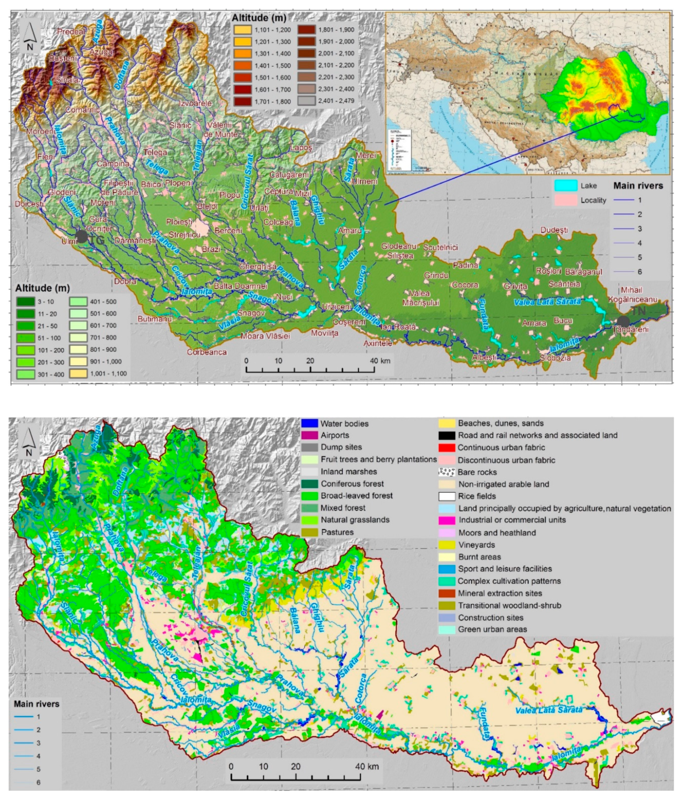
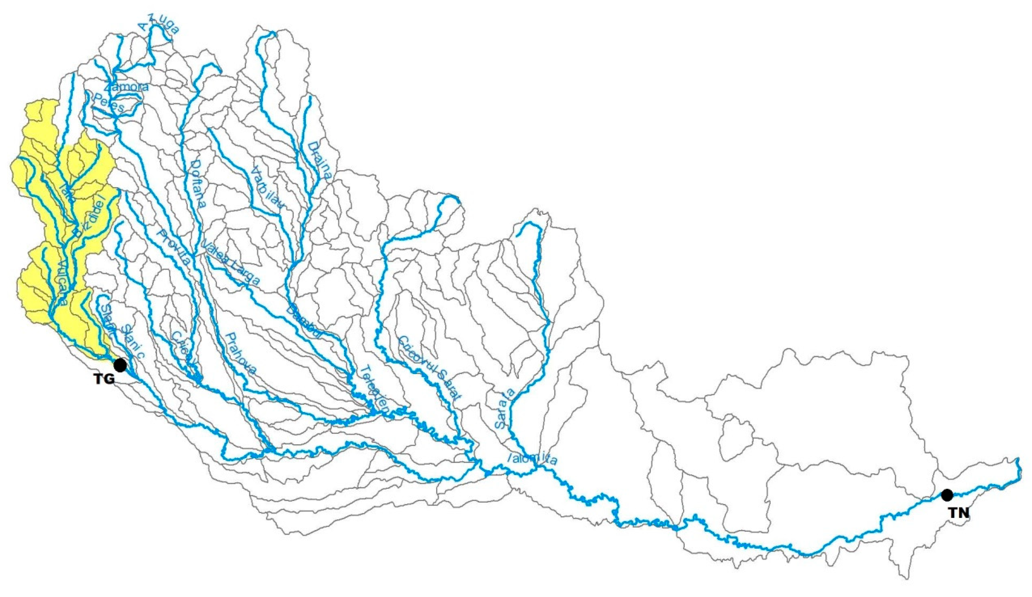
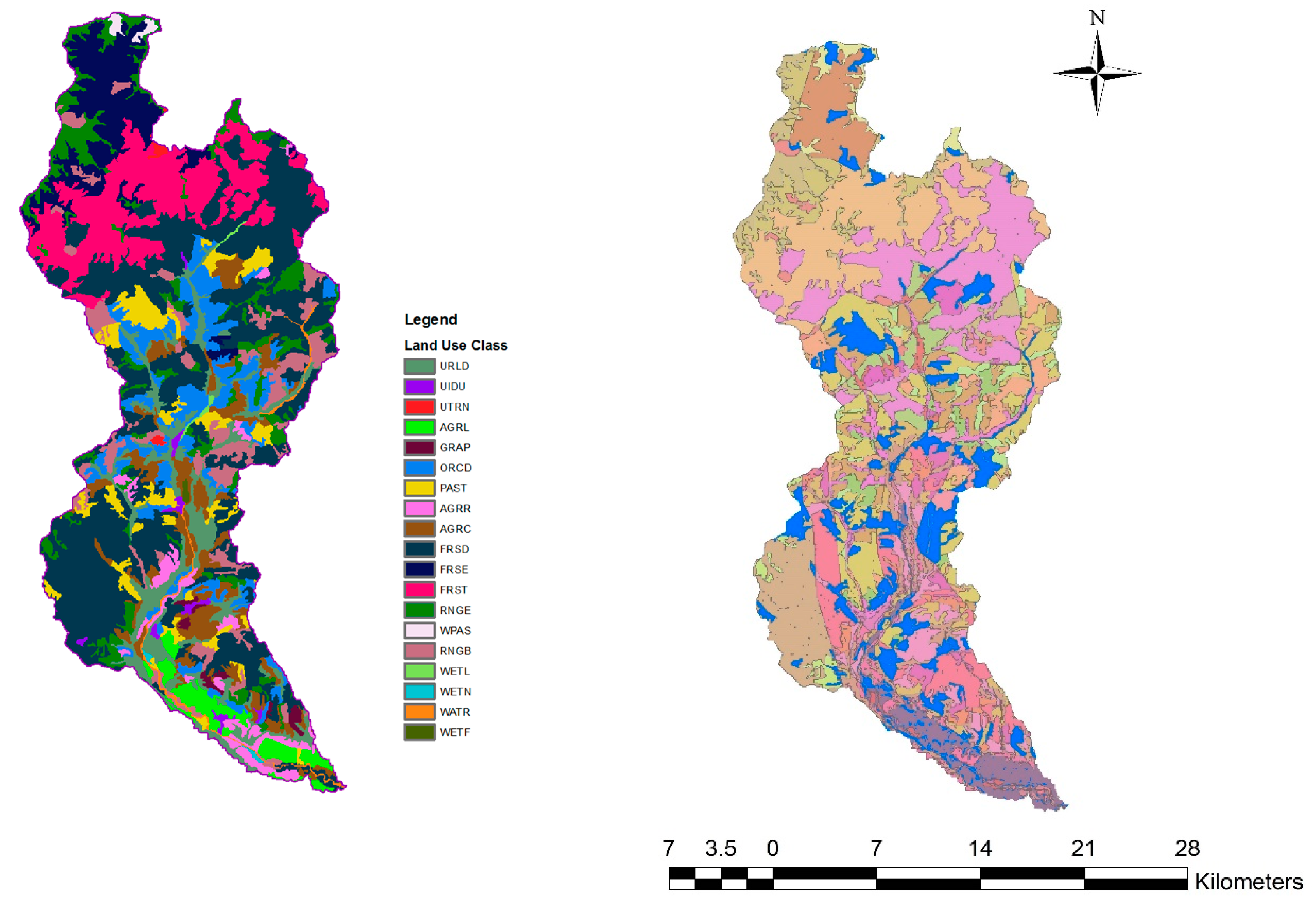
2.1. Research Area

Ialomita River has a length of 417 km and a watershed area of 10,350 km2 (4.34% of Romania’s area). The sinuosity coefficient is 1.88 with an average slope of the basin around 15 ‰. The average altitude of Ialomita River sub-basins varies from 761 m above Black Sea level (a.BS.l) at Baleni-Romania to 42 m a.BS.l at the confluence with the Danube River (Table 1) [18]. The basin has 142 coded tributaries (Figure 1). The drainage density of the Ialomita basin is 0.30 km/km2. Along the watercourse, the average multiannual discharge increases from 1 m3/s in the Bolboci area up to 40 m3/s in the Cosereni section, maintaining this value until it reaches the confluence with the Danube River (as it no longer receives any major tributary) [36]. The Prahova River is the main left tributary of the Ialomita and brings the largest discharge contribution [37] (Table 1).
Arable land predominates in the Buzau-Ialomita hydrographic area occupying 70% of the total. The next greatest proportion of the catchment is forested area (predominantly the deciduous forests), which covers 20% [38], while perennial crops cover 3% of the area. Urban and industrial areas occupy approximately 3%, each [39].
Supplementary information regarding the Ialomita River Basin were provided i.e., water management scheme (Figure S1), soil and slope maps (Figure S2), geological map (Figure S3), and soil texture map (Figure S4).
In the area of study, most runoff derived from highland and mountain massif areas and from areas where the runoff forming is under the influence of various zonal factors (lakes, karst, marshes, economic activities etc.). A close correlation exists between the relief forms and the coefficient of variation associated with the runoff. Highest runoff occurs to the tributaries on the windward slopes of the Carpathian Mountains in sub-basins situated 750 m above Black Sea level. Rivers flowing across the Romanian Plain are characterized by less runoff (in some cases less than 30 mm/year) and numerous rivers in the plain dry up during hot periods of the year. With regard to seasonal variability, the highest runoff occurs in spring (40%–50% of the annual average value). Maximum river discharge is generally recorded in April–May in rivers in mountainous regions, and in March for rivers of highlands and plains. Evaporation reduces with altitude in line with declining temperatures, while in plains evaporation is closely correlated with available soil moisture [18,19].

2.2. Monitoring of Water Physicochemical Parameters

The data monitored on Ialomita River in the control section located downstream of Tandarei hydrometric station have been recorded within the Transnational Monitoring Network of the Danube River (TNMN), International Commission for the Protection of the Danube River (ICPDR). Starting from the year 2000, the main objective of the TNMN was to assess the status of the water bodies (according to the Water Framework Directive 2000/60/EC) and, in the long term, to recover the water quality and diminish the loads of the water pollutants in the Danube River, and in its main tributaries. The review process of the TNMN was completed in 2007 with the finalization of the Report regarding the Monitoring Programs in the Danube River Basin, in which several Danube tributaries (in the upstream section of confluence with the Danube River) have started to be evaluated, including the Ialomita River (https://onlinelibrary.wiley.com/doi/book/10.1002/9781444307672).
According to the procedures for obtaining primary data for the TNMN network, the main producers of such data are the laboratories of the water management authorities (e.g., the National Administration “Romanian Waters” is responsible for the Ialomita River through the Buzau-Ialomita Water Basin Administration), which transmit the data to the Hydrological Institute from Bratislava (Slovakia). The quality of TNMN data is ensured through both laboratory-specific procedures and their participation in the ICPDR inter-comparison scheme.
Within the TNMN monitoring program, the relevant hydrological (discharge) and physico-chemical parameters are recorded. These parameters include: water temperature, suspended solids, pH, conductivity, alkalinity, total hardness, total dissolved salts, calcium, magnesium, chlorides, bicarbonates, and sulfates; oxygen regime parameters i.e., dissolved oxygen, chemical oxygen demand (COD-Cr, COD-Mn), biochemical oxygen demand (BOD5); nutrients i.e., ammonium, nitrates, nitrites, total nitrogen, ortho-phosphates, total phosphorus; heavy metals and metalloids-in dissolved form i.e., iron, manganese, arsenic, cadmium, lead, mercury, nickel, arsenic, copper, chromium, zinc; other specific pollutants i.e., anion-active detergents, hydrocarbons, phenolic index etc. For these parameters, the monitoring data are recorded with monthly frequency (12 per year).
The monitoring of the surface waters was performed on control sections located in two representative points (Targoviste-TG, and Tandarei-TN) that allowed the assessment of the general status and trends in water quality (Figure 2).
The sampling, storage and handling of water samples performed with a monthly frequency was carried out according to the current standards [40]. A comprehensive dataset was recorded between 2007 and 2016 in a control section downstream of TN, which is a TNMN monitoring point. The physicochemical parameters were determined in the laboratory using gravimetric methods (suspended solids), titrimetric/volumetric methods (alkalinity, total hardness, bicarbonates, calcium, magnesium, oxygen regime parameters, chlorides), spectrophotometric methods (nitrogen and phosphorus parameters, anion-active detergents, phenolic index, sulphates), electrochemical methods (pH, conductivity, total dissolved salts) and spectrophotometric methods of atomic absorption, respectively of atomic emission with plasma inductively coupled with mass spectrometry (heavy metals).
From this dataset, pH, ammonium (NH4-N) (mg/L), alkalinity (mmol/L), nitrates (NO3-N) (mg/L), BOD5 (mg/L), total dissolved salts (TDS) (mg/L), suspended solids (TSS) (mg/L), dissolved oxygen (DO) (mg/L), orthophosphate-phosphorus (PO4-P) (mg/L), and river discharge (m3/s) were selected for presentation in this paper.
In the upper part of the Ialomita River, pH, BOD5, DO, NO3-N and PO4-P were measured upstream and downstream of TG each month between 2016 and 2018 to assess the impact of urban wastewater discharges.

2.3. Expected Mean Concentration Model

A watershed model embedded in ArcGIS that includes surface runoff from point and non-point sources was used to facilitate the analysis of the visual output and to query new information from results. EMC values in mg/L for various land cover types were retrieved from literature [14] and assigned for Ialomita River Basin areas. Reclassification was performed using GIS features allowing the estimation of annual loadings throughout the studied watershed (Figures S5 and S6).
The pollutant load (mass/time) contribution of each cell to the downstream pollutant loading results from the product between EMC (mass/volume) and the runoff (volume/time) occurring in that cell:
L = Q × EMC × k × A
where: Q—runoff (mm y−1); EMC—expected mean concentration (mg/L); A—grid cell area; k—constant (10−6 kg-m-L/mg-mm-m3 ); L—load (kg y−1).

2.4. Soil and Water Assessment Tool (SWAT) Model

ArcGIS Interface to SWAT/Version 2012.10.21 was used to perform analysis in the upper part of the basin considering as outlet the point from the control section located downstream of TG.
SWAT works on a continuous time step having several model components, i.e., weather, hydrology, erosion, sedimentation, plant growth, nutrients, pesticides, agricultural management, and channel and reservoir routing. The SWAT model was configured to use pre-defined streams and watersheds. Based on input information that were grouped for each subcomponent basin on climate, hydrologic response units (HRU), ponds/wetlands, groundwater, and the main channel draining the sub-basin, the sediments and nutrients’ loads have been predicted for the 2016–2018 period.
The simulation of the hydrological processes in a basin uses the partitioning of the main basin into subbasins. Each subbasin contains streams, which route within the subbasin and form the stream network. The subunits of the subbasins are the HRUs, which are unique and hydrological homogeneous combinations of land use/land cover, soil type and slope characteristics. HRUs are aspatial within each subbasin. In each HRU, the hydrologic cycle, nitrogen and phosphorus cycles, and crop growth are simulated based on climatic variables, hydrology, and the agricultural management in that unit [22]. Consequently, the model calculations are made on the basis of HRUs. The river discharge and water quality indices are determined from HRU to subbasin and afterwards to the watershed outlet. The SWAT model simulates hydrology as a two-component system, comprised of land hydrology (water and pollutant loadings to channels) and channel hydrology (stream’s water quantity and quality) [23]. Three layers (digital elevation model, DEM, land cover/land use, LCLU, and soil distribution, SD) are required to perform simulations in the ArcSWAT interface.
The LCLU and soil-type layers were georeferenced using the stereographic projection (central meridian: 25°; latitude of origin: 46°) and Dealul Piscului 1970 geographic coordinate system, which describes the official cartographic projection used in Romania on the Krasovsky 1940 ellipsoid (Azimuthal Stereographic perspective oblique conform projection in secant plane 1970). The soil layer was developed from the pedological map of Romania. LCLU layer of the area was extracted from the latest CORINE land cover database. Two reservoirs were added to the model, Bolboci and Pucioasa. The topographic report for the watershed showed a minimum altitude of 232 m and a mean elevation of 763.7 m, with 53.03% coefficient of variation.
The second module of the ArcSWAT, namely HRU analysis, allowed the land use, soil, and slope definition based on soil and land cover appropriate databases. HRUs were generated using a threshold of 10%. Two reports were available for consultation: land use, soils, slope distribution, and final HRU distribution.
The weather data from the Targoviste WMO meteorological station were used in the Weather stations module, comprising daily precipitation, maximum and minimum temperature, solar radiation data, relative humidity, and wind speed data (Table S2http://worldweather.wmo.int/en/home.html). ArcSWAT simulation was performed for three years (2016–2018) allowing the assessment of nutrient loads (nitrates and phosphates) in the watershed on a monthly scale for the upper part of the basin.
SWAT-CUP, which is the calibration, validation and sensitivity analysis tool for SWAT, was applied, because it is the standard in the SWAT community for calibration (http://www.eawag.ch/forschung/siam/software/swat/index). Observed river discharge was used for calibration. SUFI2 was considered to run a sensitivity analysis at outlet (TG downstream) following the procedures described in the manual [23]). The p-factor presents the observed data fraction that is inside the 95% confidence intervals of the predictive uncertainty (p-factor needs to be close to 1). The r-factor is the width of the 95% prediction uncertainty (r-factor needs to be close to 0) [23].

2.5. Statistical Analysis

The Statistica program (Statsoft. Inc., Tulsa, OK, USA, 2007) was used to statistically analyse the recorded time series data to detect and evaluate temporal patterns in water quality and establish robust conclusions regarding the water quality trends in the Ialomita River Basin
Descriptive statistics and Pearson’s correlation were employed to identify the strength of the linear relationship between 8 variables (pH, ammonium, alkalinity, nitrates, BOD5, suspended solids, dissolved oxygen, and orthophosphate-phosphorus). Factor analysis (FA) based on normalized varimax was applied for the TN dataset to reduce the number of factors explaining variability in the model. An input matrix of 107 objects (number of recordings) by the aforementioned 8 water variables was considered. The eigenvalues that satisfied the Kaiser criterion (>1) supported the selection of three factors. Eigenvalues define the variance within the dataset accounted for by each factor. A factor with a low eigenvalue has a diminished contribution to the explanation of variances within variables and may be ignored [40].
The Hot Spot Analysis tool from ArcGIS provided the Getis-Ord Gi* statistic for each feature in the potential pollutant load dataset. This tool analyzes each feature within the context of neighboring features. A feature must have a high z-score and be surrounded by other features with high values to be a statistically significant hot spot (https://desktop.arcgis.com/en/arcmap/10.3/tools/spatial-statistics-toolbox/hot-spot-analysis.htm).

3. Results

3.1. Expected Mean Concentration (EMC) Modeling for the Ialomita River Basin

The average stream runoff of the territory under review was assessed primarily by the amount of precipitation reaching its surface and by evaporation, the two hydrometeorological factors reflected in the heat/moisture ratio (runoff ≈ 145 mm; evaporation ≈ 590 mm at Tandarei). Generally, the average specific discharge found in the Southern areas of Eastern Europe notable for relatively low amounts of precipitation and increased rates of evaporation are less than 1 L/sec km2 [12].
After merging the runoff depth with EMC values in mg/L for each land cover type (Figures S5 and S6), the estimation of multiannual loadings of suspended solids (kg/year) throughout the studied watershed was obtained (Figure 3). Four areas were clearly delineated (blue, light blue, brown, and red) with lower values of EMC in the northwestern part of the basin, which have increased towards the eastern part up to the discharge in the Danube River. The highest potential pollutant load overlaps with the large agricultural land areas located in the Romanian Plain. Figure 4 shows the results of the hot spot analysis, which supports this statement. The EMC model includes surface runoff from point and non-point sources. The main sources are represented by agriculture, human settlements, other sources (e.g., deposition of nitrogen oxides from the atmosphere), as well as the natural background. The estimated average specific emission on the total area for nitrogen was 3.2 kg N/ha, and 0.3 kg P/ha for phosphorus highly influenced by the agricultural activities.

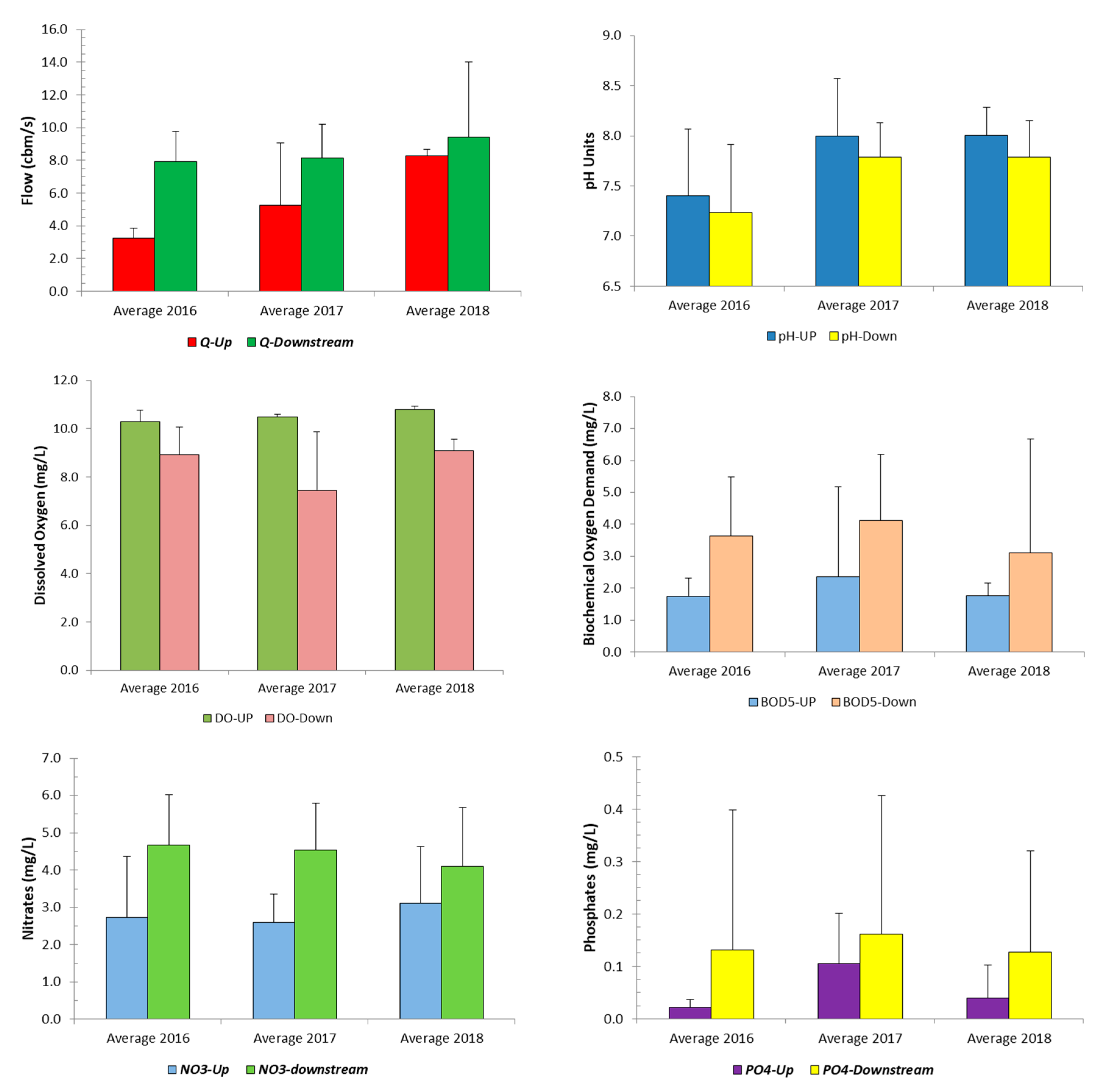
3.2. Water Quality Assessment in the Lower Part of the Ialomita River Basin

Descriptive statistics of the 10 year time series recorded downstream of TN, near the discharge of the Ialomita River in the Danube, provided an indicative synthetic image of the water quality patterns (Table 2). The highest variance was recorded for TSS and TDS followed by the river discharge, while the remaining parameters were relatively constant with low multiannual and seasonal variability.
The mean values of water parameters for 10 years monitoring in the control section that is close to the Ialomita River discharge in the Danube River were pH = 7.60 (range: 6.41–8.40), NH4-N = 1.20 mg/L (0.02–14.87), alkalinity = 4.12 mmol/L (1.34–6.27), NO3-N = 2.60 mg/L (0.08–17.30), PO4-P = 0.09 mg/L (0–0,31), DO = 8.87 mg/L (2.72–15.96), BOD5 = 5.50 mg/L (0.01–74.71), TSS = 508.32 mg/L (15.2–4457), TDS = 733.69 mg/L (455.2–1053), and river discharge = 38.60 m3/s (8.22–165). Several strong correlations (p < 0.01) were found between the tested water physicochemical variables (Table S1). Negative correlations were found between pH and ammonium, and pH and orthophosphate-phosphorus. Positive correlations occurred between ammonium and nitrates, and ammonium and orthophosphate-phosphorus, respectively. Other positive correlations have been observed between alkalinity and nitrates, and alkalinity and dissolved oxygen.
FA showed 4 factors that reached the Kaiser criterion (Table 3). These four factors explain 70.99% of the variability in the tested dataset.
After rotation, the first factor was formed by three variables i.e., pH, ammonium and orthophosphate-phosphorus (26.5% from the total variance). Factor 2 comprised alkalinity and dissolved oxygen (18.4%). The biochemical oxygen demand reached the highest factor loading (0.906) and formed the third factor (13.1%). The last factor included the total suspended solids (12.8%). Table 4 presents the factor loadings for each tested variable resulting from the varimax rotation with Kaiser normalization.

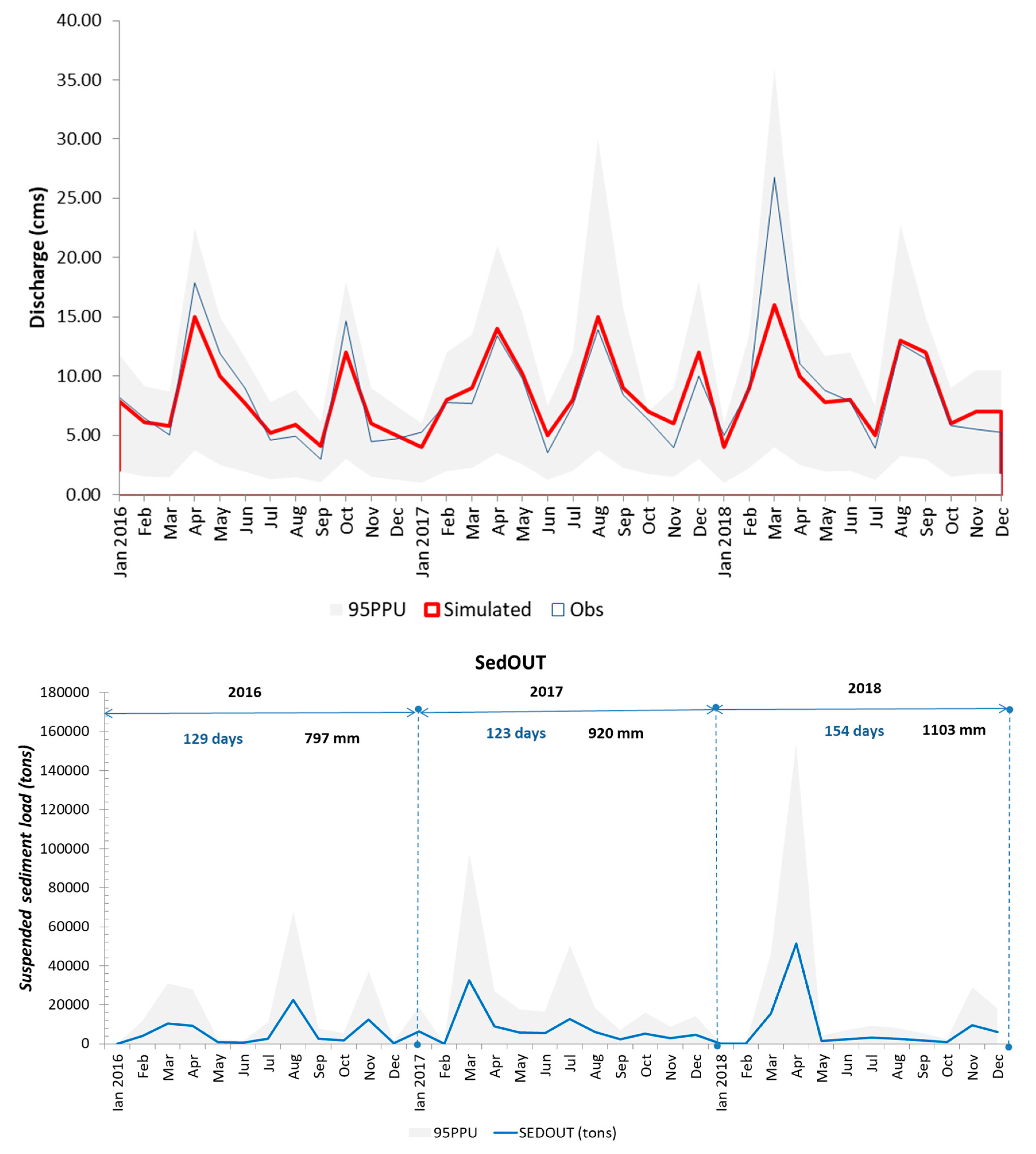
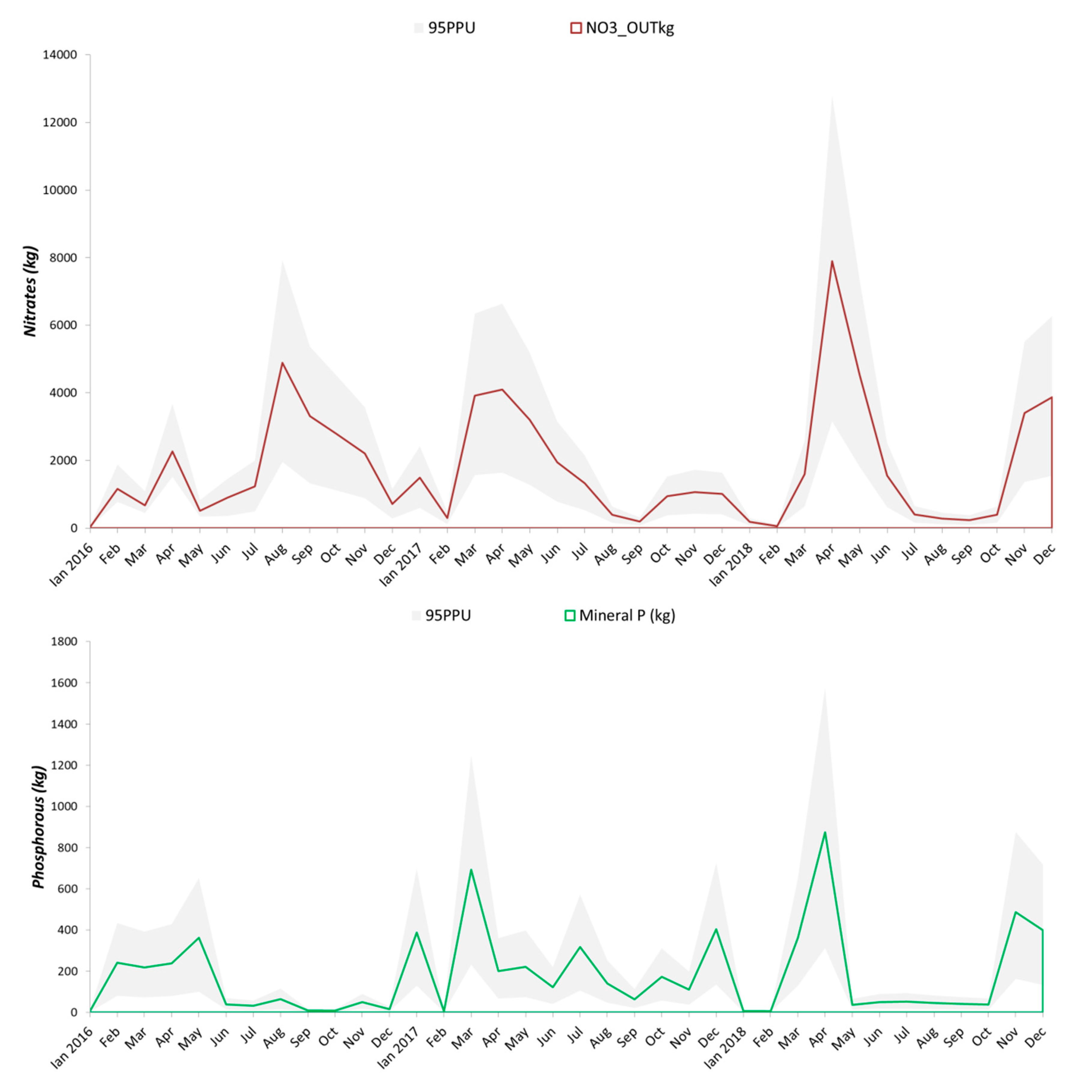
3.3. Application of SWAT Model and Water-Quality Assessment in the Upper Part of the Ialomita River Basin

The resulting HRUs have similar types of land cover, soil type, and slope characteristics and consequently comparable response to land surface processes including evapotranspiration, runoff generation, soil water interaction, lateral flow, and groundwater input [41]. These were carried out in each HRU along with water balance. Figure 5 presents the SWAT land use classes and the resultant HRU classification. SWAT identified 30 HRUs for the selected area of 67,963 ha provided in the HRU distribution report. Approximately half of this area (33,178 ha) is occupied by HRUs that contain Forest Deciduous and Forest Mixed classes in combination with various soil-type categories. Orchard and Agricultural Land-Close-grown HRUs accounted 18.2% (12,387 ha).
The simulation period ran from January 2016 to December 2018 according to the period in which water quality sampling and monitoring were performed in the control sections located near Targoviste city (Figure S7). Discharge rate, rainfall, and land use were among significant factors affecting nitrates concentrations and loads. After calibration of the discharge, the observed vs. simulated time series yielded good results (i.e., NSE = 0.77; R2 = 0.83; p-factor = 0.82 and r-factor = 0.32). Figure 6 presents the graphs based on SWAT simulation between 2016 and 2018 with the pollutant load for the reach output at downstream of TG control section for sediments, nitrates and mineral P. Based on sum of precipitation (mm), and the number of days with precipitation, the wettest year was 2018, followed by 2017 and 2016, respectively. The period with snow cover followed the same order, with 2016 being the year with the shortest period of snow cover. Consequently, the patterns provided by the model followed the weather trends. The highest amounts of sediments transported in the main channel simulated at the control outlet occurred in February–May for the years 2017 and 2018.
These periods were correlated with melting snow and precipitation, suggesting that the main contribution is from non-point sources. The same pattern corresponded to NO3-N and mineral P. During 2016, the simulated time series had a different pattern i.e., the highest quantities in July–September for sediments, and for NO3-N between July and November. This contrasting pattern could be attributed to urban wastewater discharge occurring during low river discharge periods. The annual monthly average of nitrates at the considered outlet was estimated at 1721.8 kg/month in 2016, 1657.2 kg in 2017, and 2034.2 kg in 2018, respectively.
With regard to soluble phosphorus from both diffuse and point sources, surface runoff transports organic and mineral P attached to soil particles to the main channel. Consequently, phosphorus is associated with the sediment loading from the HRU [24]. The presence of phosphates in water is a consequence of pollution with industrial wastewaters, pesticides, fertilizers, detergents, etc. This process favors water eutrophication.
Mineral P potential load was also simulated with SWAT. The monthly average concentration of mineral phosphorus at the control outlet during 2016–2018 was estimated at 106.84 (2016), 236.4 (2017), and 199.6 kg P/month (2018).
Both nitrates and phosphorus time series did not show a repeatable temporal pattern being significantly influenced by the meteorological events and river discharge.
Figure 7 shows the synthetic results of the water parameters monitoring for both control sections. While the water flow, BOD5, nitrates, and phosphates increased, pH and DO decreased, irrespective of the monitoring year, which emphasize that the water quality is worsening due to urban wastewater contributions to the pollutant load. Comparing the upstream and downstream concentrations, BOD5 increased with 52.2% (2016), 42.4% (2017), and 43.1% (2018), NO3-N 41.6%, 42.6%, and 24.3%, and PO4-P 83.4%, 34.9%, and 68.7%, respectively. Knowing the mean nitrate concentrations and converting the units combined with river discharge, the annual loads for the upstream section were estimated at 1769.04 kg (2016), 1648.8 kg (2017), and 2015.2 kg (2018). These results were close to the simulated annual pollutant loads. The index of agreement (Willmott), which is the ratio of the mean square error and the potential error, was close to 1 (0.991), a very good match. However, the nitrate loads provided by the model should be close to the downstream concentrations. This limitation originates from not including the major point sources such as WWTP and other important discharges in the river. The estimated loads based on monitored concentrations were 3026.1 kg (2016), 2935.4 kg (2017), and 2663.2 kg (2018), which are clearly higher.

4. Discussion

The latest reported official data regarding the water status of 25 water bodies—rivers monitored on a length of 1020 km in the Ialomita River Basin, pointed out that from the point of view of ecological status, 465 km (45.59%) were assessed in good ecological status and 555 km (54.41%) in moderate ecological status based on an evaluation system developed in line with the Water Framework Directive [19].
Following the observations from the monitoring and modeling of parameters in the Ialomita River Basin, water quality is influenced by the characteristics of the river basin, mainly by the land use/land cover and geology of the basin, the seasonal patterns, the river discharge, and the chemical properties of tributary water of the main channel (Figure S8). Important factors in the quantitative balance of surface waters are precipitation and snowmelt. These factors have both quantitative and qualitative influences, mainly because of surface transport of sediment, pesticides, fertilizers, etc. The resultant grouping of variables from FA suggests a significant influence of the diffuse sources coming from agricultural activities, as well as from human settlements/agglomerations (preponderantly for phosphorus emissions). Aeration conditions were represented by the next two factors. Critical conditions may occur at the interactions of physical, chemical, and biological characteristics of the receiving waters and pollutant loading sources. Such conditions can increase the adverse effects of a pollutant of concern [14]. Summer is the critical period for low dissolved oxygen and eutrophication. During this period, low river discharge and increased temperature would increase the effect of a specific pollutant load, which will have negative effects on aquatic life [35].
Current knowledge about the water cycle at basin scales is relatively incomplete due to some random and complex processes, which are difficult to measure or estimate in an integrated way. Furthermore, hydrological and water-quality data for the watercourses that form a river system are often dispersed or discontinuous, making difficult to assess the information regarding the river discharge in view of water resources management in case of flood risk or high pollutant load [37,38,39].
Numerical modeling of water quality at river basin scale must find convenient solutions by simulating potential scenarios in the catchment area that can improve the action plans to be taken in case of risk situations [42]. Such risks include prolonged periods with low discharge rates of the river and high loads of pollutants, floods, industrial accidents, accidental discharges of effluents with high loads of pollutants, polluting agricultural technologies in the river catchment area etc. Input parameters, state variables and some transformation functions must be adapted to the specific conditions of the river basin studied to increase the accuracy of models, using actual field observations and measurements, updated thematic maps, as well as information provided by the remote-sensing systems. The predictive performance of models regarding the discharge simulations considering the precision and the number of entries in the model, especially in the case of high flows, might be improved using non-parametric methods for the analysis of recorded stream hydrographs [43]. For many water-quality parameters, it is useful to sample changes through the hydrograph event, during rising stage, peak, falling stage, and baseflow [44,45].
With regard to the EMC approach, there are some limitations including not considering infiltration, interflow or groundwater processes, as well as key atmospheric conditions such as temperature or evapotranspiration. Furthermore, the EMC model uses the mean annual runoff and discharge measurements with one-time water-quality sampling data. One solution is to apply a more complex model such as SWAT, but this requires accurate data as inputs to achieve reliable results for large-scale basins. Such data are not available for the Ialomita River Basin. Consequently, we have applied the SWAT model for a smaller region of the basin to test its capabilities in providing predictions and scenarios of water quality.
The main limitations observed in the use of the SWAT model to forecast water quality in various control sections can be minimized by careful input selection and validation, optimal calibration and sensitivity analysis, and by updating the information regarding the land use/land cover, which can be obtained using remote-sensing satellite data [46].
Satellite observations succeeded to improve and update the knowledge regarding the characterization of entities and processes on the ground that are required for SWAT modeling (e.g., soil moisture, evapotranspiration, vegetation structure, and other biometric properties of the canopy such as photosynthetically active radiation (PAR), leaf area index (LAI), chlorophyll content etc. [47,48]). Remote-sensing applications also provide information to support mapping of the distribution of habitats and species [49].
Updated data regarding surface reflectance and temperature, normalized differential vegetation index (NDVI), and other related spectral indices provided by a wide variety of remote-sensing sensors have been used in numerous studies to determine the land cover and the phenology of growth and development of cultivated species or of natural ecosystems, information that can be used in SWAT model [50,51,52]. These features could be applied to improve the performances of water quality modeling and will be tested in future work to support long-term social and economic stability and sustainable development. These desiderata depend significantly on the efficient management of available water resources, respectively on the protection against depletion and degradation by acquiring updated knowledge about their status and spatiotemporal evolution.

5. Conclusions

Contamination of the river systems from anthropogenic sources is a major issue that needs to be carefully addressed. The research presented has explored several techniques for water quality assessment at a catchment scale in an integrated way including expected mean concentration and soil and water assessment tool models in conjunction with water quality assessment in the lower and upper parts of the Ialomita River Basin. The SWAT model has the capacity of detailed input information and may produce accurate predictions concerning the nitrates and phosphorus loadings at a selected outlet provided that the point sources are integrated in detail. The monitoring results showed that the pollutant load in the Ialomita River is significant due to the amount of pollutants received in the water body and has a seasonal variability. Future work will consider a more detailed description of field-scale agricultural operations at the watershed level to define better the contribution of diffuse sources to the water channel loadings. Likewise, the complexity will increase by adding the relevant point pollution sources that discharge wastewaters. The final aim of such an approach is to provide informational support to the decision-making processes regarding the improvement of the water quality in the Ialomita River Basin.

Supplementary Materials

The following are available online at https://www.mdpi.com/2073-4441/12/3/735/s1: Figure S1: Water management scheme of Ialomita River Basin, Figure S2: Soil and slope maps of Ialomita River Basin, Figure S3: Geological map of Ialomita River Basin, Figure S4: Soil texture map of Ialomita River Basin, Figure S5: Reclassification of total nitrogen (mg/L) based on land cover, Figure S6: Reclassification of total phosphorous (mg/L) based on land cover, Figure S7: Position of the two monitoring points selected to characterize the impact of urban wastewaters on the Ialomita River quality, Figure S8: Ecological status assessment of the water bodies on the Ialomita River and its tributaries, Table S1: Correlation matrix (n = 107) of the variables recorded downstream Tandarei control section on Ialomita River between 2007 and 2016, Table S2: Meteorological data recorded at Targoviste used for SWAT modeling.

Author Contributions

Conceptualization, D.D., P.B., D.T., G.S.; Data curation, E.T.; S.I.; R.T.; N.P.; Formal analysis, D.D., P.B., D.T., G.S.; Methodology, E.T.; S.I.; R.T.; N.P.; Project administration, D.D.; P.B.; D.T.; Resources, R.T.; S.I.; N.P.; E.T.; Software, D.D., P.B., D.T., G.S.; Supervision, D.D., P.B., D.T., G.S.; Validation, E.T.; S.I.; R.T.; N.P.; Writing—Original draft, D.D.; D.T.; G.S.; P.B.; Writing—Review and editing, R.T.; S.I.; N.P.; E.T.; All authors have equal contribution to the preparation of this scientific paper. All authors have read and agreed to the published version of the manuscript.

Funding

This work was supported by a grant of the Romanian National Authority for Scientific Research, CNDI– UEFISCDI, project number PN-III-1.2-PCCDI-2017-0721.

Acknowledgments

The authors want to thank the editor and the four anonymous reviewers whose comments have contributed to the improvement of the original manuscript and Michael Reid from University of New England for the English language proofing and useful suggestions.

Conflicts of Interest

The authors declare no conflict of interest.

References

  1. UN-Water. Towards a Worldwide Assessment of Freshwater Quality—A UN-Water Analytical Brief 2016. Available online: https://www.unwater.org/app/uploads/2017/05/UN_Water_Analytical_Brief_20161111_02_web_pages.pdf (accessed on 20 December 2019).
  2. Borchardt, D.; Bogardi, J.J.; Ibisch, R.B. (Eds.) Integrated Water Resources Management: Concept, Research and Implementation; Springer: Basel, The Switzerland, 2016; p. 781. [Google Scholar]
  3. Stoner, E.W.; Albrey Arrington, D. Nutrient inputs from an urbanized landscape may drive water quality degradation. Sustain. Water Qual. Ecol. 2017, 9–10, 136–150. [Google Scholar] [CrossRef]
  4. Amblard, L. Collective action for water quality management in agriculture: The case of drinking water source protection in France. Glob. Environ. Chang. 2019, 58, 101970. [Google Scholar] [CrossRef]
  5. Szopińska, M.; Szumińska, D.; Polkowska, Ż.; Machowiak, K.; Lehmann, S.; Chmiel, S. The chemistry of river–lake systems in the context of permafrost occurrence (Mongolia, Valley of the Lakes). Part I. Analysis of ion and trace metal concentrations. Sediment. Geol. 2016, 340, 74–83. [Google Scholar] [CrossRef]
  6. Kosek, K.; Polkowska, Ż. Determination of selected chemical parameters in surface water samples collected from the Revelva catchment (Hornsund fjord, Svalbard). Mon. für Chem.-Chem. Mon. 2016, 147, 1401–1405. [Google Scholar] [CrossRef] [Green Version]
  7. Popa, C.L.; Bretcan, P.; Radulescu, C.; Carstea, E.M.; Tanislav, D.; Dontu, S.I.; Dulama, I.D. Spatial distribution of groundwater quality in connection with the surrounding land use and anthropogenic activity in rural areas. Acta Montan. Slovaca 2019, 24, 73–87. [Google Scholar]
  8. Melland, A.R.; Fenton, O.; Jordan, P. Effects of agricultural land management changes on surface water quality: A review of meso-scale catchment research. Environ. Sci. Policy 2018, 84, 19–25. [Google Scholar]
  9. Dunea, D.; Iordache, S.; Radulescu, C.; Pohoata, A.; Dulama, I.D. A multidimensional approach to the influence of wind on the variations of particulate matter and associated heavy metals in Ploiesti City, Romania. Rom. J. Phys. 2016, 61, 1354–1368. [Google Scholar]
  10. Costache, A.; Sencovici, M. Influence of the socio-demographic variables on environmental perception. Case study: Targoviste (Dambovita county, Romania). In Proceedings of the 15th International Multidisciplinary Scientific Geoconference (SGEM) Ecology, Economics, Education and Legislation, Albena, Bulgaria, 18–24 June 2015; Volume I, pp. 431–438. [Google Scholar]
  11. Sencovici, M.; Costache, A. Methods and means of evaluating the perception concerning the environmental condition. Case study: The urban ecosystem of Targoviste (Romania). Int. Multidiscip. Sci. GeoConference: SGEM: Surv. Geol. Min. Ecol. Manag. 2012, 5, 571. [Google Scholar]
  12. FAO. The State of the World’s Land and Water Resources for Food and Agriculture (Solaw)—Managing Systems at Risk; Food and Agriculture Organization of the United Nations: Rome and Earthscan: London, UK, 2011. [Google Scholar]
  13. Ruman, M.; Polkowska, Ż.; Zygmunt, B. Processes and the Resulting Water Quality in the Medium-Size Turawa Storage Reservoir after 60-Year Usage. Water Qual. 2017, 377. [Google Scholar] [CrossRef] [Green Version]
  14. Syed, A.T.; Jodoin, R.S. Estimation of nonpoint-source loads of total nitrogen, total phosphorous, and total suspended solids in the Black, Belle, and Pine River basins, Michigan, by use of the PLOAD model. In U.S. Geological Survey Scientific Investigations Report 2006-5071; U.S. Geological Survey, 1 December 2016; 42p, Available online: https://doi.org/10.3133/sir20065071 (accessed on 20 December 2019).
  15. Zeleňáková, M.; Harabinová, S.; Mésároš, P.; Abd-Elhamid, H.; Purcz, P. Modelling of Erosion and Transport Processes. Water 2019, 11, 2604. [Google Scholar] [CrossRef] [Green Version]
  16. Dunea, D.; Iordache, Ş. Time series analysis of the heavy metals loaded wastewaters resulted from chromium electroplating process. Environ. Eng. Manag. J. (EEMJ) 2011, 10, 469–482. [Google Scholar]
  17. Echeverría, C.; Guiomar, R.-P.; Puertes, C.; Samaniego, L.; Barrett, B.; Francés, F. Assessment of Remotely Sensed Near-Surface Soil Moisture for Distributed Eco-Hydrological Model Implementation. Water 2019, 11, 2613. [Google Scholar] [CrossRef] [Green Version]
  18. National Administration of Romanian Waters. The Management Plan of The Buzau-Ialomita Hydrographic Area. Available online: http://www.rowater.ro/ (accessed on 20 December 2019).
  19. Romanian Ministry of the Environment; Aquaproiect, S.A. The Atlas of Water Cadaster from Romania; Romanian Ministry of the Environment: Bucuresti, Romania, 1992. (In Romanian)
  20. Dunea, D.; Tanislav, D.; Stoica, A.; Bretcan, P.; Muratoreanu, G.; Frasin, L.N.; Alexandrescu, D.; Iliescu, N. ECO-PRACT: A project for developing the research competences of students regarding the monitoring of floristic composition in mountain grasslands. J. Sci. Arts 2018, 18, 225–238. [Google Scholar]
  21. Diaconu, D.C.; Andronache, I.; Ahammer, H.; Ciobotaru, A.M.; Zelenakova, M.; Dinescu, R.; Pozdnyakov, A.V.; Chupikova, S.A. Fractal drainage model-a new approach to determinate the complexity of watershed. Acta Montan. Slovaca 2017, 22, 12–21. [Google Scholar]
  22. Neitsch, S.L.; Arnold, J.G.; Kiniry, J.R.; Williams, J.R. Soil and Water Assessment Tool Theoretical Documentation, Version 2009. Temple, Texas Water Resources Institute: USDA-ARS Grassland, Soil and Water Research Laboratory, 2011. Available online: http://swat.tamu.edu/media/99192/swat2009-theory.pdf (accessed on 20 December 2019).
  23. Abbaspour, K.C. SWAT-CUP 2012. SWAT Calibration and Uncertainty Program—A User Manual, 2013. Available online: https://swat.tamu.edu/media/114860/usermanual_swatcup.pdf (accessed on 20 December 2019).
  24. Dunea, D.; Iordache, Ş.; Pohoaţă, A.; Cosmin, M. Prediction of nutrient loads from wastewater effluents on Ialomita River water quality using SWAT model support. Ann. Food Sci. Technol. 2013, 14, 356–365. [Google Scholar]
  25. Wang, R.; Yuan, Y.; Yen, H.; Grieneisen, M.; Arnold, J.; Wang, D.; Wang, C.; Zhang, M. A review of pesticide fate and transport simulation at watershed level using SWAT: Current status and research concerns. Sci. Total Environ. 2019, 669, 512–526. [Google Scholar] [CrossRef]
  26. Chun, J.A.; Baik, J.; Kim, D.; Choi, M. A comparative assessment of SWAT-model-based evapotranspiration against regional-scale estimates. Ecol. Eng. 2018, 122, 1–9. [Google Scholar] [CrossRef]
  27. Francesconi, W.; Srinivasan, R.; Pérez-Miñana, E.; Willcock, S.P.; Quintero, M. Using the Soil and Water Assessment Tool (SWAT) to model ecosystem services: A systematic review. J. Hydrol. 2016, 535, 625–636. [Google Scholar] [CrossRef]
  28. Niraula, R.; Kalin, L.; Srivastava, P.; Anderson, C.J. Identifying critical source areas of nonpoint source pollution with SWAT and GWLF. Ecol. Model. 2013, 268, 123–133. [Google Scholar] [CrossRef]
  29. Naramngam, S.; Tong, S.T.Y. Environmental and economic implications of various conservative agricultural practices in the Upper Little Miami River basin. Agric. Water Manag. 2013, 119, 65–79. [Google Scholar] [CrossRef]
  30. Sommerlot, A.R.; Nejadhashemi, A.P.; Woznicki, S.A.; Prohaska, M.D. Evaluating the impact of field-scale management strategies on sediment transport to the watershed outlet. J. Environ. Manag. 2013, 128, 735–748. [Google Scholar] [CrossRef] [PubMed]
  31. Einheuser, M.D.; Nejadhashemi, A.P.; Woznicki, S.A. Simulating stream health sensitivity to landscape changes due to bioenergy crops expansion. Biomass Bioenergy 2013, 58, 198–209. [Google Scholar] [CrossRef]
  32. Shrestha, N.K.; Leta, O.T.; De Fraine, B.; van Griensven, A.; Bauwens, W. OpenMI-based integrated sediment transport modelling of the river Zenne, Belgium. Environ. Model. Softw. 2013, 47, 193–206. [Google Scholar]
  33. Santra, P.; Das, B.S. Modeling runoff from an agricultural watershed of western catchment of Chilika lake through ArcSWAT. J. Hydro-Environ. Res. 2013. [Google Scholar] [CrossRef]
  34. Kim, J.; Choi, J.; Choi, C.; Park, S. Impacts of changes in climate and land use/land cover under IPCC RCP scenarios on streamflow in the Hoeya River Basin, Korea. Sci. Total Environ. 2013, 452–453, 181–195. [Google Scholar] [CrossRef] [PubMed]
  35. Luo, Y.; Ficklin, D.L.; Liu, X.; Zhang, M. Assessment of climate change impacts on hydrology and water quality with a watershed modeling approach. Sci. Total Environ. 2013, 450–451, 72–82. [Google Scholar] [CrossRef] [PubMed]
  36. Bălteanu, D.; Micu, D.; Costache, A.; Diana, D.; Persu, M. Socio-economic vulnerability to floods and flash-floods in the bend subcarpathians, Romania. Int. Multidiscip. Sci. GeoConference Surv. Geol. Min. Ecol. Manag. 2015, 1, 577–584. [Google Scholar]
  37. Oprea, M.; Dunea, D. SBC-MEDIU: A multi-expert system for environmental diagnosis. Environ. Eng. Manag. J. (EEMJ) 2010, 9, 205–213. [Google Scholar]
  38. Diaconu, D.C.; Andronache, I.; Pintilii, R.-D.; Bretcan, P.; Simion, A.G.; Draghici, C.C.; Gruia, K.A.; Grecu, A.; Marin, M.; Peptenatu, D. Using fractal fragmentation and compaction index in analysis of the deforestation process in Bucegi Mountains Group, Romania. Carpathian J. Earth Environ. Sci. 2019, 14, 431–438. [Google Scholar]
  39. Costache, A.; Sencovici, M.; Murarescu, O. Land use and land cover change in Dambovita county, Romania (1990–2012). In Proceedings of the 14th SGEM GeoConference on Ecology, Economics, Education and Legislation, Albena, Bulgaria, 19–25 June 2014; Volume 1, pp. 405–412, ISBN 978-619-7105-17-9. [Google Scholar]
  40. Water Quality Standards: SR EN ISO 5667-1: 2007, Water Quality. Sampling. Part 1: General Guide for Establishing Programs and Sampling Techniques; SR EN ISO 5667-3: 2013, Water Quality. Sampling. Part 3: Conservation and Handling of Water Samples; SR ISO 5667-6/1997, Water Quality. Sampling. Part 6: Guide for Sampling of Rivers and Streams; SR EN ISO 5667-6: 2017, Water Quality. Sampling. Part 6: Guide for Sampling of Rivers and Streams; SR EN ISO 5667-14: 2017, Water Quality. Sampling. Part 14: Guide for Quality Assurance and Quality Control in the Collection and Treatment of Water in the Environment. Available online: https://www.iso.org/publication-list.html (accessed on 20 December 2019).
  41. Panda, U.C.; Sundaray, S.K.; Rath, P.; Nayak, B.B.; Bhatta, D. Application of factor and cluster analysis for characterization of river and estuarine water systems—A case study: Mahanadi River (India). J. Hydrol. 2006, 331, 434–445. [Google Scholar] [CrossRef]
  42. Wang, P.; Yao, J.; Wang, G.; Hao, F.; Shrestha, S.; Xue, B.; Peng, Y.; Xie, G. Exploring the application of artificial intelligence technology for identification of water pollution characteristics and tracing the source of water quality pollutants. Sci. Total Environ. 2019, 693, 133440. [Google Scholar] [CrossRef] [PubMed]
  43. Patil, A.; Ramsankaran, R. Improving streamflow simulations and forecasting performance of SWAT model by assimilating remotely sensed soil moisture observations. J. Hydrol. 2017, 555, 683–696. [Google Scholar] [CrossRef]
  44. Petrow, T.; Merz, B. Trends in flood magnitude, frequency and seasonality in Germany in the period 1951–2002. J. Hydrol. 2009, 371, 129–141. [Google Scholar] [CrossRef] [Green Version]
  45. Dunea, D.; Iordache, Ş. An analysis of high flows from stream hydrographs of Ialomita River at Targoviste gauge station. Ann. Food Sci. Technol. 2014, 14, 154–161. [Google Scholar]
  46. Ma, T.; Duan, Z.; Lia, R.; Song, X. Enhancing SWAT with remotely sensed LAI for improved modelling of ecohydrological process in subtropics. J. Hydrol. 2019, 570, 802–815. [Google Scholar] [CrossRef] [Green Version]
  47. Luan, X.; Wu, P.; Sun, S.; Wang, Y.; Gao, X. Quantitative study of the crop production water footprint using the SWAT model. Ecol. Indic. 2018, 89, 1–10. [Google Scholar] [CrossRef]
  48. Romagnoli, M.; Portapila, M.; Rigalli, A.; Maydana, G.; Burgués, M.; García, C.M. Assessment of the SWAT model to simulate a watershed with limited available data in the Pampas region, Argentina. Sci. Total Environ. 2017, 596–597, 437–450. [Google Scholar] [CrossRef] [Green Version]
  49. Franklin, J. Mapping Species Distributions—Spatial Inference and Prediction; Cambridge University Press: Cambridge, UK, 2009. [Google Scholar]
  50. Glenn, E.P.; Neale, C.M.U.; Hunsaker, D.J.; Nagler, P.L. Vegetation index-based crop coefficients to estimate evapotranspiration by remote sensing in agricultural and natural ecosystems. Hydrol. Process. 2011, 25, 4050–4062. [Google Scholar] [CrossRef]
  51. Gonzalez-Dugo, M.P.; Escuin, S.; Cano, F.; Cifuentes, V.; Padilla, F.L.M.; Tirado, J.L.; Oyonarte, N.; Fernandez, P.; Mateos, L. Monitoring evapotranspiration of irrigated crops using crop coefficients derived from time series of satellite images. II. Application on basin scale. Agric. Water Manag. 2013, 125, 92–104. [Google Scholar] [CrossRef]
  52. Vuolo, F.; Żółtak, M.; Pipitone, C.; Zappa, L.; Wenng, H.; Immitzer, M.; Atzberger, C.; Weiss, M.; Baret, F. Data service platform for Sentinel-2 surface reflectance and value-added products: System use and examples. Remote Sens. 2016, 8, 938. [Google Scholar] [CrossRef] [Green Version]
Figure 1. Hydrographical network and land cover in Ialomita River Basin (Source of data: https://www.danubecommission.org/uploads/images/Duna-2009-1-1-000-000-2500-.jpg and https://land.copernicus.eu/pan-european/corine-land-cover/clc2018).
Water 12 00735 g001
Figure 2. Monitoring points of water quality (dots) and the yellow area for soil and water assessment tool (SWAT) modeling considered for this study (other areas represent the composing sub-basins of Ialomita River Basin).
Water 12 00735 g002
Figure 3. Potential pollutant load—suspended solids (TSS, kg/year) resulted from the expected mean concentration (EMC) model.
Water 12 00735 g003
Figure 4. Hot spot analysis of the potential pollutant load Ialomita River Basin.
Water 12 00735 g004
Figure 5. SWAT land use classes and the hydrologic response units (HRU) generated by SWAT model (yellow area in Figure 2).
Water 12 00735 g005
Figure 6. SWAT simulation showing the pollutant load for the reach output (TG downstream) between 2016 and 2018—river discharge, sediments (SED_OUT: Sediment transported with water out of reach in metric tons), nitrates and mineral P; sum of precipitations (mm), number of days with precipitations; 95% prediction uncertainty (95PPU).
Water 12 00735 g006aWater 12 00735 g006b
Figure 7. River flow, pH and water quality parameters in the upper part of the Ialomita River Basin upstream and downstream of Targoviste city; error bars represent standard deviation.
Water 12 00735 g007
Table 1. Multiannual hydrological parameters recorded in various control sections of Ialomita River Basin and its major tributary Prahova River (see water management scheme—Figure S1); a.BS.l—above Black Sea level.
No.RiverHydrometric StationWatershed Area
F (km2)
Watershed Average Altitude H (m a.BS.l)Hydrological Parameters
Multi-Annual Average Discharge QmmaMaximum Discharge at 1% Probability Qmax 1%Suspended Sediment Discharge R
(m3/s)(m3/s)(kg/s)
1IalomitaBaleni-Romani (downstream Targoviste9017619.1777016.1
2IalomitaSilistea Snagovului (before Dridu reservoir)192051512.487015.8
3PrahovaAdancata (near the confluence with Ialomita River)368254927.31165113
4IalomitaCosereni (near Urziceni)626549042.71730102
5IalomitaSlobozia915436541.776563
Table 2. Statistical indicators of the hydrological parameters recorded in the control section of Tandarei from the Ialomita River Basin (2007–2016); TSS—total suspended solids, DO—dissolved oxygen, and TDS—total dissolved salts.
VariablepHNH4-NAlkalinityNO3-NBOD5TSSDOPO4-PDischargeTDS
Unit-mg/Lmmol/Lmg/Lmg/Lmg/Lmg/Lmg/Lm3/smg/L
Mean7.601.204.122.605.50508.328.870.0938.60733.69
Std. Error of Mean0.050.180.080.170.7268.730.230.003.4413.95
Median7.700.254.002.123.58243.508.900.0832.70731.00
Std. Deviation0.482.300.892.117.67824.752.480.0629.00138.10
Variance0.235.310.804.4758.81680,211.96.150.00841.1019,070.7
Skewness−0.773.410.323.216.803.150.271.262.000.23
Std. Error of Skewness0.230.190.230.200.230.200.220.200.290.24
Kurtosis−0.1913.880.8615.9758.8710.460.132.275.04−0.50
Std. Error of Kurtosis0.450.390.450.390.450.400.440.390.560.48
Range1.9914.854.9317.2274.714441.8013.240.31156.78597.80
Minimum6.410.021.340.080.0115.202.720.008.22455.20
Maximum8.4014.876.2717.3074.714457.0015.960.311651053
Table 3. Factor extraction based on eigenvalues: principal components (Kaiser criterion >1).
FactorEigenvalue% Total VarianceCumulative%
12.12126.51526.515
21.47218.40144.916
31.05513.18958.105
41.03112.88970.994
Table 4. Rotated component matrix extraction method: principal component analysis; rotation method: varimax with Kaiser normalization—marked loadings are >0.70 (rotation converged in 6 iterations)—Tandarei dataset.
VariableComponent
1234
pH−0.7750.039−0.0890.158
NH4-N0.7330.2820.3410.082
Alkalinity0.0330.847−0.2440.058
NO3-N0.4120.5030.2980.428
BOD50.032−0.0810.906−0.052
TSS−0.178−0.123−0.0630.837
DO−0.120.7280.137−0.334
PO4-P0.709−0.127−0.223−0.053

