A Combination Model for Quantifying Non-Point Source Pollution Based on Land Use Type in a Typical Urbanized Area

Abstract

Water pollution poses threats to urban environments and subsequently impacts the ecological health and sustainable development of urban areas. Identifying the spatiotemporal variation in non-point sources (NPS) pollution is a prerequisite for improving water quality. This paper aimed to assess the NPS pollution load and then recognized the spatiotemporal characteristics of the pollution sources in a typical urbanized area. A combination model based on land use type was used to simulate the NPS pollution load. The results showed the following: (1) ponds and farmlands had higher pollution production intensities than other land use types, but the intensity and magnitude of pollution emissions were generally greater in urban areas; (2) monthly and annual total nitrogen (TN) and total phosphorus (TP) emissions had the same pattern as rainfall, and TN and TP emissions accounted for 56.2% and 58.0%, respectively, of the total in summer; (3) TN pollution was more serious than TP pollution in the study area, especially in farmlands; (4) urban runoff (UR) and livestock and poultry breeding (LPB) were the main sources of NPS, TN and TP emissions in the study area. If these NPS pollutants cannot be removed from this area, a large amount of freshwater is needed to dilute the current rivers to meet the requirement of the fourth category of China national environmental quality standards for surface water. This problem is serious in the control of polluted rivers in many cities throughout China.

1. Introduction

China has experienced rapid urbanization since the 1990s [1]. Unfortunately, urban population growth and land use changes have led to the degradation of flowing watercourses and the discharge of excessive wastewater [2]. Such water pollution, which threatens drinking water, agricultural irrigation and the ecological landscape, has become a key issue restricting urban development [3]. Consequently, the Chinese government has regarded urban water pollution with great importance and has invested substantial amounts of energy and money accordingly [4,5]. Nevertheless, some cities still face serious water pollution problems, especially rapidly developing cities where land use patterns are changing fast and sewage management and treatment are lacking [6,7,8]. To further control and improve the water quality situation in such cities, accurately recognizing of the sources of pollutants is of considerable significance.

In general, water pollution is caused mainly by point sources and non-point sources (NPS) pollution. The former, such as industrial and domestic pollution, is relatively easy to collect into the pipe networks and process in the sewage treatment facilities, whereas the latter, which is widely distributed and originates from multiple-source, is more difficult to monitor and control and has tremendous impact on the water quality of lakes and rivers [9,10,11]. Appropriately, many studies have focused on the assessment of NPS pollution loads. The most common and concerning sources of NPS pollution primarily include urban runoff (UR) [12], agricultural runoff (AR) [13], livestock and poultry breeding (LPB) [14] and aquaculture [15]. Ongley et al. [13] estimated the pollution statuses of agricultural and rural areas and their contribution to the total water pollution throughout China. Li et al. [16] simulated the NPS pollution load in the city of Baoding and analysed the effects of NPS pollution on Baiyangdian Lake. Due to the complexity of NPS components, empirical methods are often used to comprehensively evaluate all NPS pollutants, but these methods broadly lack detailed spatial and temporal descriptions [11]. Some studies have attempted to simulate the temporal variation in and the spatial distribution of pollutants, but most research has focused mainly on a certain type of NPS pollution, such as UR or AR [8,17,18]. In addition, because LPB and aquaculture do not correspond exactly to a specific type of land use, their spatial distributions are relatively difficult to describe [15,19,20,21].

Accurate estimations of NPS pollution are important for the processing of NPS pollution loads [3,13,16]. The most common methods for evaluating NPS pollution loads include empirical evaluation methods and physics-based models [17,22]. The export coefficient model, which is based on a number of statistical materials to calculate pollution load, is the most common empirical method [23]. The methodology behind the export coefficient model is easy to understand, but this approach relies heavily on the accuracy of the empirical data and cannot explain the dynamic processes responsible for generating the pollution loads. Moreover, the use of empirical data rather than real-time data means that the results obtained using this method usually have a large time step (monthly, seasonal or annual). In contrast, physical-based models are employed primarily to establish the relationship of rainfall runoff pollution loads and simulate the NPS pollution loads during the rainfall runoff process [7,24]. These models generally contain good physical mechanisms, and some can provide information regarding the spatial and temporal distribution characteristics of NPS pollution loads [7,8,12]. Some common NPS models are shown in

Table 1. Some commonly used physical-based non-point source (NPS) models.

Model	Name	Applicability	Advantages	Disadvantages
AGNPS [25]	Agricultural Non-Point Source	Rainstorm events and continuous monitoring for watersheds	Strong water quality simulation mechanism; the various sources of pollutants are clearly described	Many parameters need to be determined; large quantities of data are needed
HSPF [26]	Hydrological Simulation Program-Fortran	Rainstorm events and continuous monitoring for watersheds and urban areas	Better capture the detailed runoff and water quality processes	Lacking detailed spatial descriptions; limitations in urban areas
SWAT [27]	Soil and Water Assessment Tool	Continuous monitoring for watersheds	Master the long-term effects of land management measures on water, sediment and pollution; low data requirements	Not applicable to simulations finer than daily scale; parameters need to be adjusted in different regions
SWMM [18,26,28]	Storm Water Management Model	Rainstorm events and continuous monitoring for urban areas and watersheds	Complete modules and good applicability; suitable for pipe network simulations	Highly demanding parameters; limitations in watersheds
STORM [17]	Storage, Treatment, Overflow, Runoff Model	Rainstorm events and continuous monitoring for urban areas	Easy to use	Cannot simulate the migration and transformation of pollutants

.

Most of these models described above are expert in simulating specific pollution sources or pollutions of certain land use patterns. Urban rainstorm events are often the focus of attention in urban areas; for this purpose, models such as SWMM and STORM are commonly used [18,26,28]. Additionally, some models, such as SWAT and HSPF, are well suited to the evaluation of NPS pollution in a watershed or farmland [17,27,29], but are not applicable to urbanized areas. These NPS evaluation models generally encounter problems with insufficient water quantity or quality modules. Lee et al. [26] compared the water quality simulation effects of SWMM and HSPF in urban areas and found that SWMM is suitable for almost only urban areas, whereas HSPF can be applied to only homogenous land uses. Some studies have tried to improve upon existing models or to couple multiple models to form a new model; the resulting models can acquire better simulation results in diversified land use patterns. Lin et al. [30] assessed the effects of NPS phosphorus on soil by integrating the sediment delivery distributed (SEDD) and pollution load (PLOAD) models. Yang et al. [31] coupled the Xinanjiang model and SWAT to assess the NPS pollution load around Songtao Reservoir on Hainan Island. Nevertheless, land uses in urbanized areas encompass the characteristics of both urban and rural areas, and, thus, a variety of NPS types need to be considered. In addition, most of these models were developed in the United States or Europe; hence, considering the climate and soil distribution differences between these regions and China and other regions, some improvements must be implemented when using these models.

This study investigated a typical urbanized area, the Dafeng Basin. The study area has experienced rapid development with an urban population which has more than doubled in recent decades, but little attention has been paid to the water pollution therein, which seriously affects the quality of people’s lives and hinders sustainable social and economic development within the basin. The most problematic pollutant is domestic sewage, although NPS pollution is also significant; both sources aggravate the existing burden on the water environment. In recent years, the local government has increased its investments in water pollution control and management; however, measured data from monitoring sites shows that despite the many measures that have already been implemented, the levels of TN and TP pollutants still do not meet the requirement of water quality standards (GB 3838-2002 standard in China). Since there is no TN standard for rivers in this standard, we use ammonia nitrogen standard to replace it. In this study, we evaluated the spatiotemporal dynamics of NPS pollution of the Dafeng Basin. On the basis of an evaluation of the previous literature, no model was found to be completely applicable to this type of region. Therefore, we combined multiple lumped models to develop an NPS assessment model that would be well suited to the study area. The main NPS pollutants in the study area were considered, including UR, AR, LPB, aquaculture and others, and their connections with land use were established. The combined model consists of two modules: water quantity and water quality, focusing on TN and TP, and considering the dynamic simulation of pollutant accumulation and erosion of pollutants under different land use conditions. Via the proposed model based on land use type, the spatiotemporal variation in the NPS pollution load were simulated and used to provide a scientific basis for regional water pollution control.

2. Study Area and Materials

2.1. Study Area

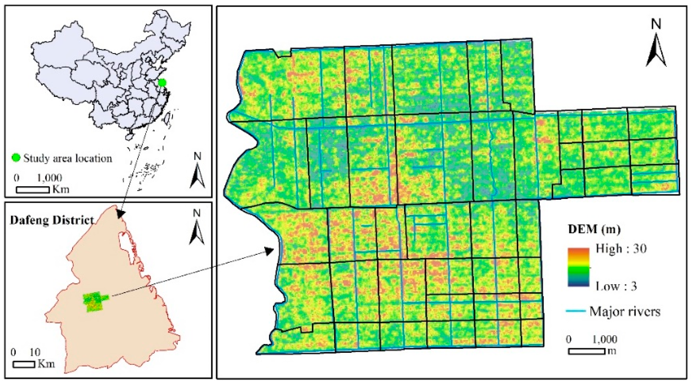
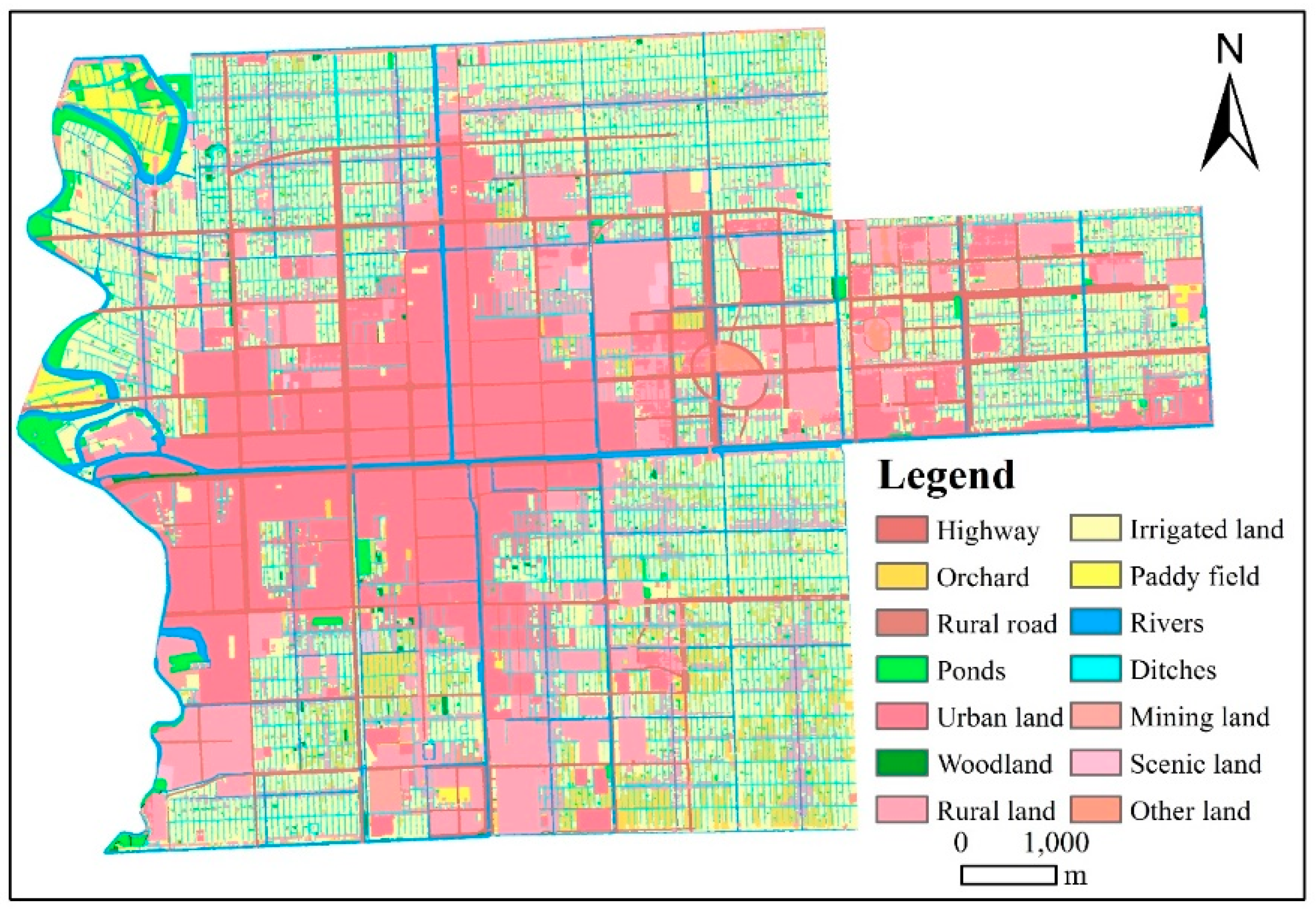
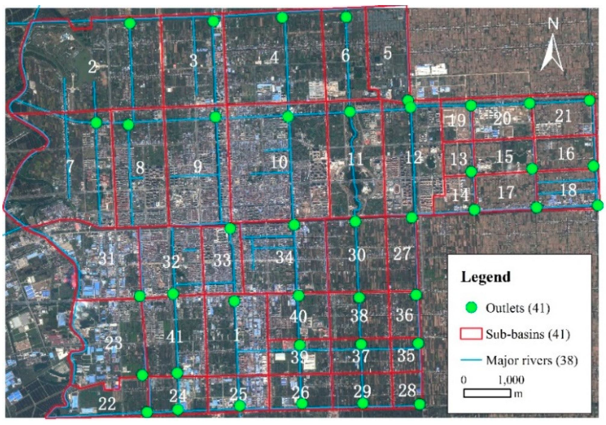
The study area is a typical urbanized basin that covers an area of approximately 74.6 km² with a permanent population of about 185 thousand, of which has nearly 82.9% were urban residents in 2019. This area includes the urban area of Dafeng District and its surrounding suburbs, which border the Yellow Sea to the east (Figure 1). The terrain is very flat; the elevation is relatively high, at 10.24 m, in the south and relatively low, at 8.79 m, in the north. The soil types in the study area are all moist soil, and most rivers have been channelized. According to the land use data in 2018 (Figure 2), the proportion of urban area (including urban land and highway) in the study area was 27.5%, while rural areas (including rural land and rural road) accounted for 19.5%, cultivated field (including irrigated land and paddy field) accounted for 30.5%, and other land use types accounted for 22.5%. The climate of this area, which is suitable for the growth of thermophilic crops, belongs to the transition zone between the subtropical and warm temperate zones. According to data acquired in the last 60 years, the average annual rainfall is 1075 mm, and the average annual evaporation was approximately 800 mm. The precipitation from June to September accounts for 63% of the precipitation throughout the whole year. In 2017, the average annual temperature was 15.7 °C, the daily maximum temperature was 38.6 °C and the daily minimum temperature was −6.8 °C. A true-colour image showing the distribution of sub-basins is provided in Figure 3.

2.2. Data Used in this Study

All input data employed for the NPS simulations included the following: (1) meteorological data from the period 2000 to 2018, including precipitation and evaporation; (2) vector data on land use types (Figure 2) and hydrographic networks (Figure 3); (3) watershed data obtained manually using digital elevation model (DEM) data and high-resolution imagery (Figure 3); (4) soil type distributions and relevant parameters were from the China Soil Characteristics Dataset (CSCD) [32]; (5) discharge of industrial pollutants, release of endogenous pollutants, and domestic pollutants and loss of NPS pollutants obtained from on-line monitoring data, laboratory test data and field survey data, respectively; and (6) socioeconomic data obtained from local governmental statistical yearbooks. The data and their sources are summarized in

Table 2. Data and their sources.

Data Type	Scale	Data Description	Data Source
Meteorological data	Daily and Hourly	Precipitation and evaporation	Dafeng station, from the National Meteorological Information Center
Land use types	1:50,000	Vector data	Local government departments
Hydrographic networks	-	Vector data	Local government departments
Soil properties	1:1,000,000	Raster data	China Soil Characteristics Dataset
Watershed data	-	Vector data, manually obtained using DEM data and high-resolution imagery	ASTER Global DEM (GDEM) data and a panchromatic multi-spectral image taken in September 2018 from the Gaofen-2 satellite
Pollution source	-	Discharge of industrial pollutants; release of endogenous pollutants; domestic pollutants, loss of NPS pollutants	On-line monitoring data from local government departments; laboratory test data; field survey data
Socioeconomic data	-	Population, industrial structure, LPB volume, etc.	Statistical yearbooks

.

3. Methods for Simulating NPS Pollutants

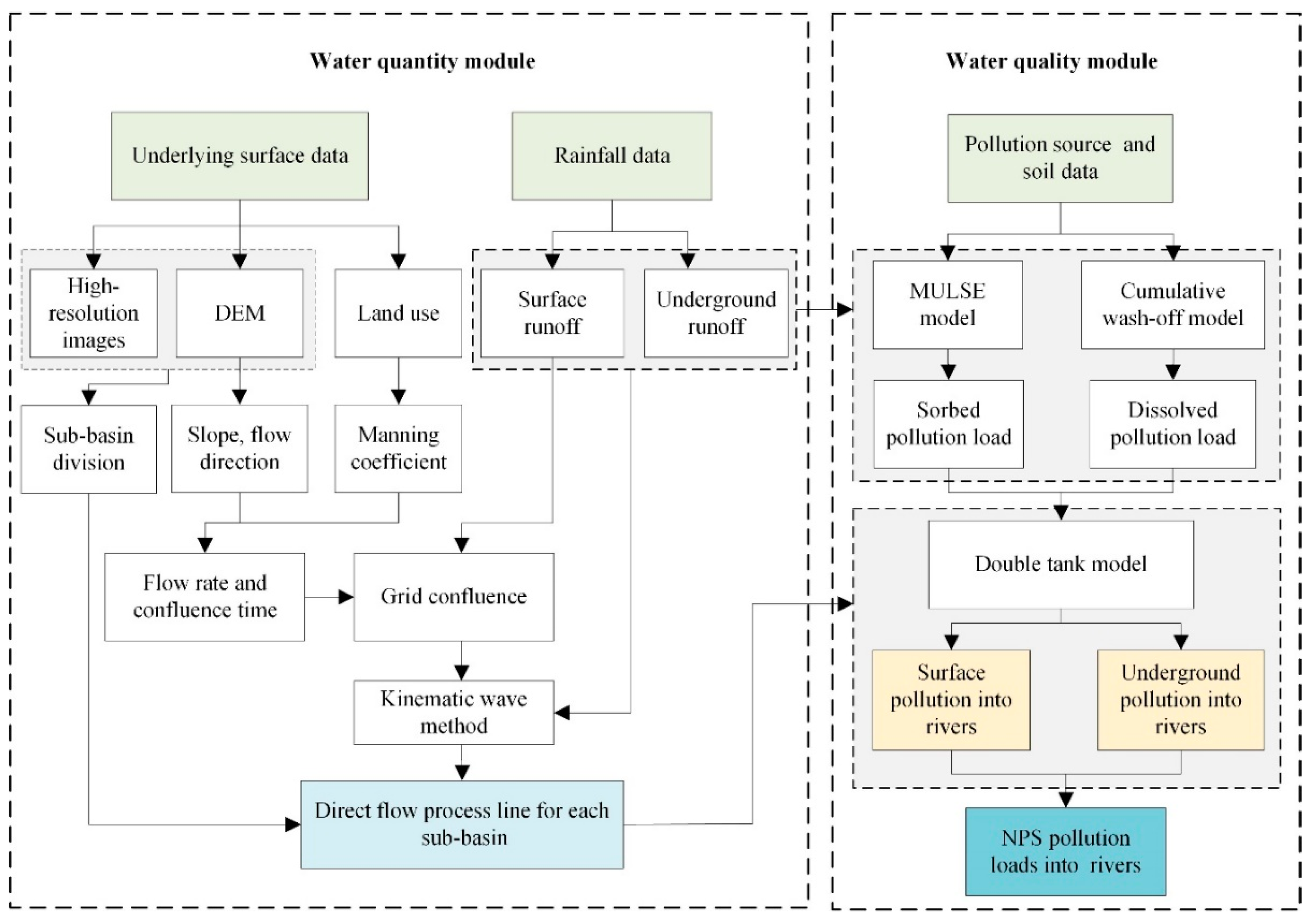
The combination model is a spatial distribution model (Figure 4). The main modules include the water quantity module, which describes the processes of runoff yield and flow concentration, and the water quality module, which depicts the processes responsible for the generation of pollutants and their discharge into rivers.

3.1. Water Quantity Module

(1) Runoff yield

Runoff was simulated according to different types of underlying surfaces. There were three main types: permeable soil, impervious surface and water surface.

For permeable soil, the grid-based Xinanjiang model was used to simulate runoff. The Xinanjiang model can be applied to runoff simulations for soil [33,34,35], but it is not suitable for impervious surfaces and water surfaces [31,35].

Impermeable surface does not consider infiltration, using the complete runoff yield method. The formula used is expressed as follows:

$${\mathrm{R}}_{\mathrm{y}}=\{\begin{array}{c}P-\mathrm{K}·\mathrm{EI}, P\ge \mathrm{K}·\mathrm{EI}\\ 0, P<\mathrm{K}·\mathrm{EI}\end{array}$$

(1)

where ${\mathrm{R}}_{\mathrm{y}}$ is the runoff yield (mm); P is the rainfall amount (mm); $\mathrm{K}$ is the evapotranspiration conversion coefficient; and EI is the evaporation measured from the evaporating dish (mm).

The water tank model, where runoff generation occurs only after the water tank is full, was used for water surfaces. The formula is as follows:

$${\mathrm{R}}_{\mathrm{y}}=\{\begin{array}{c} 0, W_t\le \mathrm{WM}\\ W_t-\mathrm{WM}, W_t>\mathrm{WM}\end{array}$$

(2)

where $W_t$ is the water storage at the end of time t. WM represents the saturated water storage, and its formula is as follows:

$$W_t=\{\begin{array}{c}{\displaystyle {\displaystyle \sum }_{i=1}^t}{\mathrm{PE}}_t+W_0, {\displaystyle {\displaystyle \sum }_{i=1}^t}{\mathrm{PE}}_t+W_0\le \mathrm{WM}\\ \mathrm{WM}, {\displaystyle {\displaystyle \sum }_{i=1}^t}{\mathrm{PE}}_t+W_0>\mathrm{WM}\end{array}$$

(3)

where $W_0$ is the initial water storage and ${\mathrm{PE}}_t$ is the net rainfall (rainfall minus evaporation) at the end of time t.

Parameter values of the runoff yield simulation in the model are shown in the

Table 3. The runoff yield simulation parameters in the combined model.

No.	Parameter	Value	Details
1	WM	(20,80,50)	Tensile water capacity, upper, lower and deep layers (mm)
2	W0	(0,75,50)	Initial water content (mm)
3	B	0.1	Water storage capacity curve index
4	S	5	Watershed average free water storage depth (mm)
5	SM	15	Average free water storage capacity in the basin (mm)
6	EX	1.6	Free water storage capacity curve index
7	KG	0.35	Outflow coefficient of free water storage to groundwater
8	KSS	0.35	Outflow coefficient of free water storage to interflow
9	KKG	0.995	Recession constant of groundwater storage
10	KKSS	0.99	Recession constant of interflow storage
11	K	0.95	Evaporation dish evaporation coefficient
12	C	0.16	Evapotranspiration coefficient of the deep layer
13	IMP	(0.5,0.7,1,0)	Impervious rate (rural and scenic land, 0.5; urban, 0.7; rural roads and highways, 1; others, 0)

.

(2) Flow concentration

The flow concentration process consists of grid confluences and sub-basin confluences. The confluence of a grid is related to the grid size; when the grid size is small, the confluence time is very short, and the confluence process could be ignored. In this paper, the grid size is 30 m. Therefore, we assumed that the grid confluence is equal to its runoff yield. The sub-basin confluence was divided into two parts: the surface and subsurface confluences. The kinematic wave method was used to calculate the confluence time for the surface runoff [36], while the water tank model was used for the subsurface runoff. For each sub-basin, the cumulative time from each grid to the sub-basin outlet was calculated as follows:

$$\Delta t={\mathrm{L}}^{0.6}·{\mathrm{n}}^{0.6}·i_c{}^{-0.4}·{\mathrm{S}}_{\mathrm{l}}{}^{-0.3}$$

(4)

where $\Delta t$ is the duration when the flow of the i-th grid reaches the outlet of the corresponding sub-basin (the value is an integer) (s); L is the ground flow length (m); n is the roughness (the values of different land use types are derived from some references and are shown in

Table 4. Relevant parameters of land use.

No.	Land Use Types	n	Cvm	M	kN	kP	FNS	FPS
1	Rivers	0.080	0	0	0	0	0.4	0.5
2	Paddy field	0.040	0.18	0.01	0.01	0.008	0.4	0.5
3	Ditches	0.080	0	0	0	0	0.4	0.5
4	Ponds	0.080	0	0	0	0	0.4	0.5
5	Irrigated land	0.040	0.31	0.50	0.04	0.048	0.7	0.8
6	Rural	0.015	0.02	0.80	0.04	0.048	0.2	0.3
7	Urban land	0.015	0.01	0.70	0.10	0.080	0.1	0.2
8	Rural road	0.015	0	0.90	0.12	0.096	0.1	0.2
9	Highway land	0.015	0	0.90	0.12	0.096	0.1	0.2
10	Mining land	0.055	0.05	0.90	0.04	0.048	0.4	0.5
11	Scenic land	0.015	0.02	0.90	0.08	0.064	0.4	0.5
12	Orchard	0.040	0.10	0.16	0.04	0.048	0.7	0.8
13	Woodland	0.200	0.10	0.16	0.04	0.048	0.7	0.8
14	Other land	0.200	0.30	0.35	0.04	0.048	0.7	0.8

[37,38]); $i_c$ is the net rain intensity (m/s); and ${\mathrm{S}}_{\mathrm{l}}$ is the slope.

According to the above formula, the surface runoff in each period through the outlets of the sub-basin was calculated as follows:

$$R_{cs}={\displaystyle \sum }_{i=1}^{\mathrm{I}}{q}_s\left(i,t-\Delta t\right)/\left({\mathrm{A}}_t·1000\right)$$

(5)

where $R_{cs}$ is the surface runoff into the river (mm); $q_s$ is unit line of surface flow (m³ s⁻¹); I is the number of all grids in the sub-basin; ${\mathrm{A}}_t$ is the total area of the basin (km²).

3.2. Water Quality Module

(1) Pollutant generation

The pollution load generated during the rainfall process includes two states: the sorbed and the dissolved. In this paper, we simplified the exchange potential between sorbed and dissolved phases.

The sorbed pollution load originates predominantly from soil erosion.

$${\mathrm{W}}_{\mathrm{so}}=S_{\mathrm{ed}}·C_n·E_r$$

(6)

where ${\mathrm{W}}_{\mathrm{so}}$ is the generated sorbed NPS pollution load (tons); $S_{\mathrm{ed}}$ is the sediment load in the surface runoff (tons); and $C_n$ is the nitrogen or phosphorus nutrient content in the soil (g/g). $E_{\mathrm{r}}$ is the enrichment factor, which was calculated as follows:

$$E_{\mathrm{r}}=0.78·{\left(\frac{S_{\mathrm{ed}}}{10·\mathrm{A}·R_{\mathrm{s}}}\right)}^{-0.2468}$$

(7)

where A is the grid area (hm²); and $R_{\mathrm{s}}$ is the surface runoff depth (mm).

Soil erosion was calculated using the Modified Universal Soil Loss Equation (MUSLE).

$$S_{\mathrm{ed}}=11.8·{\left(R_{\mathrm{s}}·q_{\mathrm{p}}·\mathrm{A}·10000\right)}^{0.56}·{\mathrm{K}}_{\mathrm{e}}·C_{\mathrm{vm}}·\mathrm{M}·{\mathrm{L}}_{\mathrm{s}}·C_{\mathrm{d}}$$

(8)

where $q_{\mathrm{p}}$ is the peak flow (m³ s⁻¹); ${\mathrm{K}}_{\mathrm{e}}$ is the soil erodibility factor; $C_{\mathrm{vm}}$ is the vegetation cover and management factor; M is the maintenance measure factor; ${\mathrm{L}}_{\mathrm{s}}$ is the topographic factor; and $C_d$ is the coarse debris factor. ${\mathrm{K}}_{\mathrm{e}}$ and $C_{\mathrm{d}}$ were calculated with soil data, whereas Ls was calculated with DEM and slope data. The determinations of $C_{\mathrm{vm}}$ and M were referred mainly to other research results and an actual investigation of the study area (Table 4).

In addition, the processes responsible for generating dissolved pollution of AR, UR and LPB are closely related to precipitation. Aquaculture pollution directly flows into the river, and thus has a minimal relationship with precipitation. The NPS pollution driven by precipitation was calculated using the cumulative wash-off model. The original cumulative wash-off model assumes that, during a rainfall period, the pollution load source is continuously attenuated during the rainfall process.

$${\mathrm{SS}}_i={\mathrm{SS}}_{i-1}·e^{-\mathrm{k}·R{c}_{i-1}}$$

(9)

where ${\mathrm{SS}}_i$ indicates the source intensity of the field rainfall at the i-th moment (tons km⁻²); k is the ground wash coefficient, including the ground wash coefficients of TN and TP (k_N and k_P) (Table 4); and $R{c}_{i-1}$ is the cumulative runoff depth (mm) at the i-th moment of the rainfall event.

As rainfall continues to fall on the field, the pollutant concentration decays exponentially with runoff depth.

Due to the influence of pollutant recharge, pollution sources accumulate. For urban area and LPB, the source of the grid pollutants will change at different times during the rainfall process. For farmland, the source of grid pollutants is replenished during both rainfall process and the dry (field drainage) period. Because the dominant pollution load is discharged during storm events, we ignore the dry period in this paper. The source of the pollutants at the i-th moment is therefore as follows:

$${\mathrm{SS}}_i=\left({\mathrm{SS}}_{i-1}+l_{i-1}·t\right)·e^{-k·R{c}_{i-1}}$$

(10)

where $l_{i-1}$ is the pollutant replenishment source at time i-1 (tons km⁻² h⁻¹).

Then, the amount of pollution at the i-th time is as follows:

$${\mathrm{Wdi}}_i={\mathrm{SS}}_{i-1}+l_{i-1}-{\mathrm{SS}}_i$$

(11)

where ${\mathrm{Wdi}}_i$ is the dissolved pollution load generated at the i–th time. AR, UR and LPB were all calculated using this method, and the total amount of pollution was calculated as follows:

$${\mathrm{Wdis}}_{ij}={\mathrm{Wdi}}_{ij}·\mathrm{A}/100$$

(12)

where ${\mathrm{Wdis}}_{ij}$ is the dissolved pollution load in a grid (tons); j is the type of NPS pollution (UR, AR and LPB); ${\mathrm{Wdi}}_{ij}$ is the pollution load per unit area of type j at the i-th time (tons km⁻²).

(2) Pollutant emissions into a river

The NPS pollution emissions entering a river are closely related to the confluence. For a single grid, the uniform water tank model was used to calculate the surface water and groundwater pollutant concentrations. For the t-th time (t $\ge 1)$:

$$\mathrm{VS}\left(t\right)=\mathrm{VS}\left(t-1\right)+\mathrm{Qs}\left(t\right)-\mathrm{qs}\left(t\right)·3.6/{\mathrm{A}}_{\mathrm{s}}$$

(13)

$$\mathrm{VG}\left(t\right)=\mathrm{VG}\left(t-1\right)+\mathrm{Q}\left(t\right)-\mathrm{Qs}\left(t\right)-\left(q\left(t\right)-\mathrm{qs}\left(t\right)\right)·3.6/{\mathrm{A}}_{\mathrm{s}}$$

(14)

$$\mathrm{CS}\left(t\right)=\frac{\mathrm{VS}\left(t-1\right)·\mathrm{CS}\left(t-1\right)+\mathrm{Trj}\left(t\right)·\mathrm{Qs}\left(t\right)/Q\left(t\right)+\mathrm{Txf}\left(t\right)}{\mathrm{VS}\left(t\right)}·\frac{1000}{{\mathrm{A}}_{\mathrm{s}}}$$

(15)

$$\mathrm{CG}\left(t\right)=\frac{\mathrm{VG}\left(t-1\right)·\mathrm{CG}\left(t-1\right)+\mathrm{Trj}\left(t\right)·\left(1-Q\mathrm{s}\left(t\right)/Q\left(t\right)\right)}{\mathrm{VG}\left(t\right)}·\frac{1000}{{\mathrm{A}}_s}$$

(16)

where VS and VG are the surface water and groundwater storage capacities, respectively (mm); Q and Qs are the total runoff and surface runoff, respectively (mm); q and qs are the total outflow and surface discharge, respectively (m³ s⁻¹); CS is the concentration of TN or TP in the surface water (mg L⁻¹); CG is the concentration of TN or TP in the groundwater (mg L⁻¹); and Trj and Txf are the production of sorbed nitrogen or phosphorus and dissolved nitrogen or phosphorus, respectively (tons); ${\mathrm{A}}_s$ is the area of each sub-basin (km²). The initial VS, VG, CS and CG were set in the model.

Settling, volatilization and degradation occur during the migration and transformation of pollutants. According to the processing module of the distributed waste load model (DWLM) [39], a processing unit can be generalized into five types: sewage treatment plant, sewer, purification tank, surface water and soil (or underground) water. Drawing upon this idea, this study considered two basic types of surface water and groundwater. The treatment coefficients were adjusted according to the types of land use—that is, the purification rates of the pollutants.

$$T=(\left(1-\mathrm{FS}\right)·{\displaystyle \sum }_i^I\mathrm{qs}\left(i,t-\Delta t\right)·\mathrm{CS}\left(i\right)+\left(1-\mathrm{FG}\right)·\mathrm{CG}·\left(q-qs\right))·3.6/{\mathrm{A}}_{\mathrm{s}}$$

(17)

where T is the amount of pollutants into the river (tons); FS (including FNS and FPS of TN and TP respectively) is the treatment coefficient of surface water, and the treatment coefficients of the different land use types differed (Table 4). FG (including FNG and FPG of TN and TP respectively) was the groundwater treatment coefficient, and FNG and FPG were set to 0.85 and 0.95, respectively.

4. Results

4.1. Rationality Analysis of the Simulation Results

(1) Simulation results of water quantity and quality

Table 5. Annual average simulation results for rainfall-based runoff from the period 2000–2018.

Parameter	Urban Land	Farmland	Other	Overall
R (mm)	873.89	428.13	473.90	585.69
RS (mm)	851.39	324.60	443.85	512.37
E (mm)	231.14	692.03	632.53	524.64
C	0.79	0.39	0.43	0.51
CS	0.77	0.29	0.40	0.47
ΔR (mm)	−1.11	−14.01	−0.30	−4.19

shows the results of the runoff simulation in the study area from 2000 to 2018. The average annual precipitation was 1100.8 mm. The soil water storage difference between the final and initial moment was 5.3 mm. ΔR represents the water balance error and the ratio of ΔR to P was less than 5%, which means that the simulation results satisfied the water balance. The total runoff coefficient was 0.51, and the surface runoff coefficient was 0.47. The surface runoff coefficient and total runoff coefficient both followed the same order: urban land > other > farmland.

Annual average simulation results of NPS pollution production from the period 2000–2018 are shown in

Table 6. Annual average simulation results of NPS pollution production from the period 2000–2018.

Type		Urban Land	Farmland	Other	Overall
Load (tons year−1)	Sediment	106.82	1169.67	145.21	1421.70
	Sorbed nitrogen	1.13	9.27	1.28	11.68
	Sorbed phosphorus	0.65	4.23	0.85	5.73
	Dissolved nitrogen	14.82	56.86	5.27	76.95
	Dissolved phosphorus	3.84	6.56	1.18	11.58
Load modulus (tons km−2 year−1)	Sediment	5.19	45.41	5.14	19.06
	Sorbed nitrogen	0.05	0.36	0.05	0.16
	Sorbed phosphorus	0.03	0.16	0.03	0.08
	Dissolved nitrogen	0.72	2.21	0.19	1.03
	Dissolved phosphorus	0.19	0.25	0.04	0.16
Area (km2)		20.59	25.76	28.24	74.58

. From the perspective of soil erosion, the study area was only slightly eroded, and the amount of farmland erosion was the largest. These results are consistent with the spatial distribution data of soil erosion in China, which was provided by Data Center for Resources and Environmental Sciences, Chinese Academy of Sciences (RESDC) (http://www.resdc.cn). Dissolved nitrogen and phosphorus were the main pollution sources, accounting for 86.8% and 66.9% of the total, respectively. Compared with that of sorbed nitrogen, the proportion of sorbed phosphorus was relatively higher, reaching 33.1%.

(2) Analysis of the rationality of the results in 2018

Table 7. All pollution loads emission into rivers in 2018.

Type		TN	TP
Point sources pollutants (tons)	Domestic pollution	243.67	18.79
	Industrial pollution	2.57	2.56
NPS pollutants (tons)	UR	14.22	3.55
	LPB	9.90	0.86
	AR	5.56	0.75
	Other	3.10	1.16
Endogenous release pollutants (tons)		−8.42	8.13
Total (tons)		270.58	35.80

shows the results of the various types of pollution loads in 2018. Among them, pollution load was calculated based on multi-source data. Domestic pollution load was obtained mainly from field survey data. The industrial pollution load was derived from on-line monitoring data provided by local government departments. The endogenous release pollution load was referred to laboratory test data; and the NPS load was simulated by the proposed combination model.

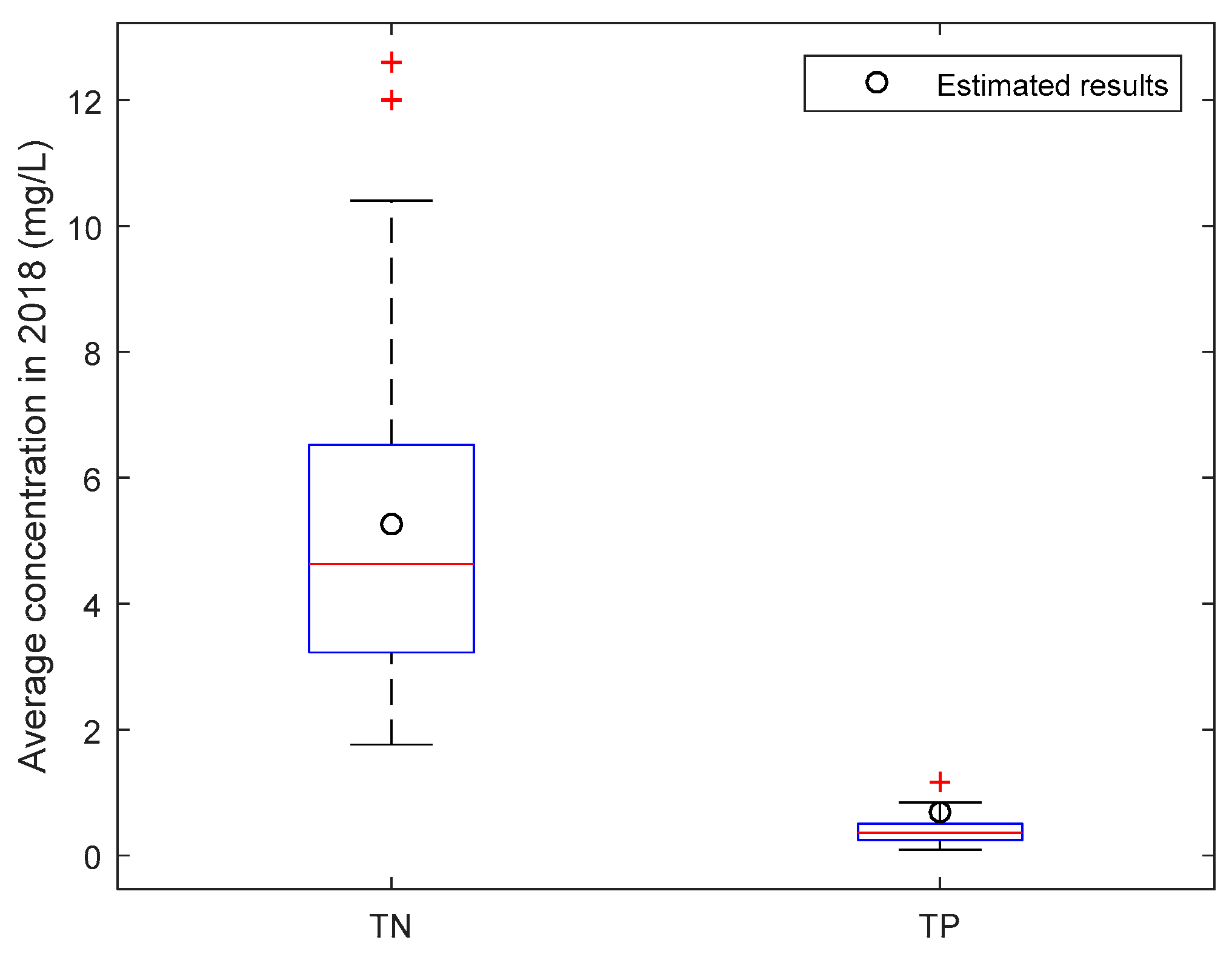
In the study area, the annual local water volume and the annual external water supply in 2018 were 4.71 × 10⁷ m³ and 4.21 × 10⁶ m³, respectively. Based on the data and the results of all pollution loads emission into rivers, we estimated that the annual average of TN and TP concentration were 5.27 mg L⁻¹ and 0.70 mg L⁻¹, respectively, in 2018. These estimated TN and TP concentrations were between the measured values and slightly above the median (Figure 5), and hence the estimated concentrations were considered reasonable.

(3) Comparison of the simulation results between two methods

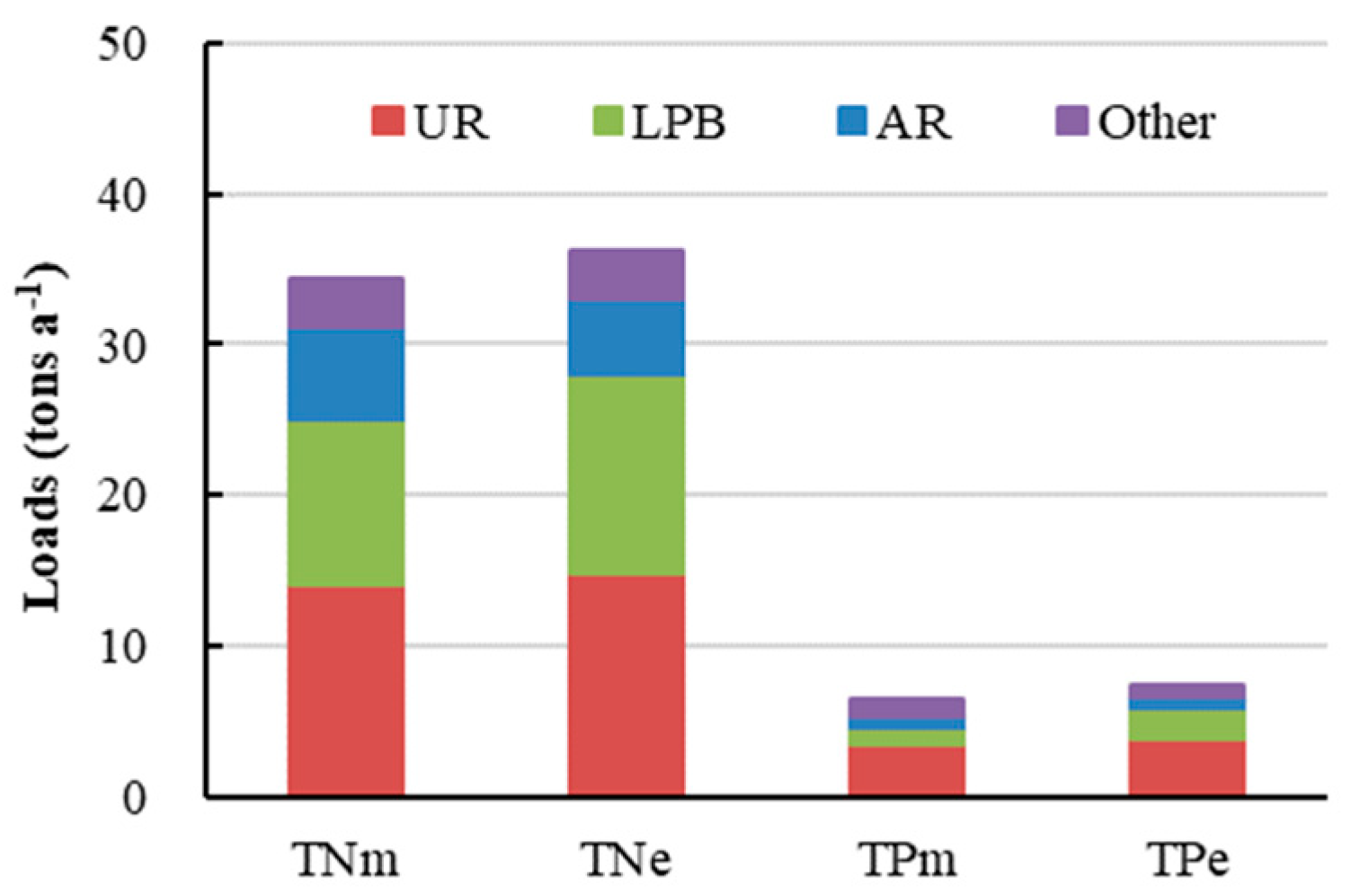
We used the export coefficient model, which is the most common method for estimating NPS pollution, to analyse the rationality of the results from the combination model. The annual average simulation results of NPS pollution emissions into rivers from the combination model and the export coefficient model were consistent regarding both the order of magnitude and the load distribution (Figure 6). The TN and TP differences between the two results were -1.99 tons and −0.44 tons, respectively; their relative errors were less than 10% of the simulation results for the total amount and for each component.

4.2. Spatial Distribution of the Simulated NPS Loads

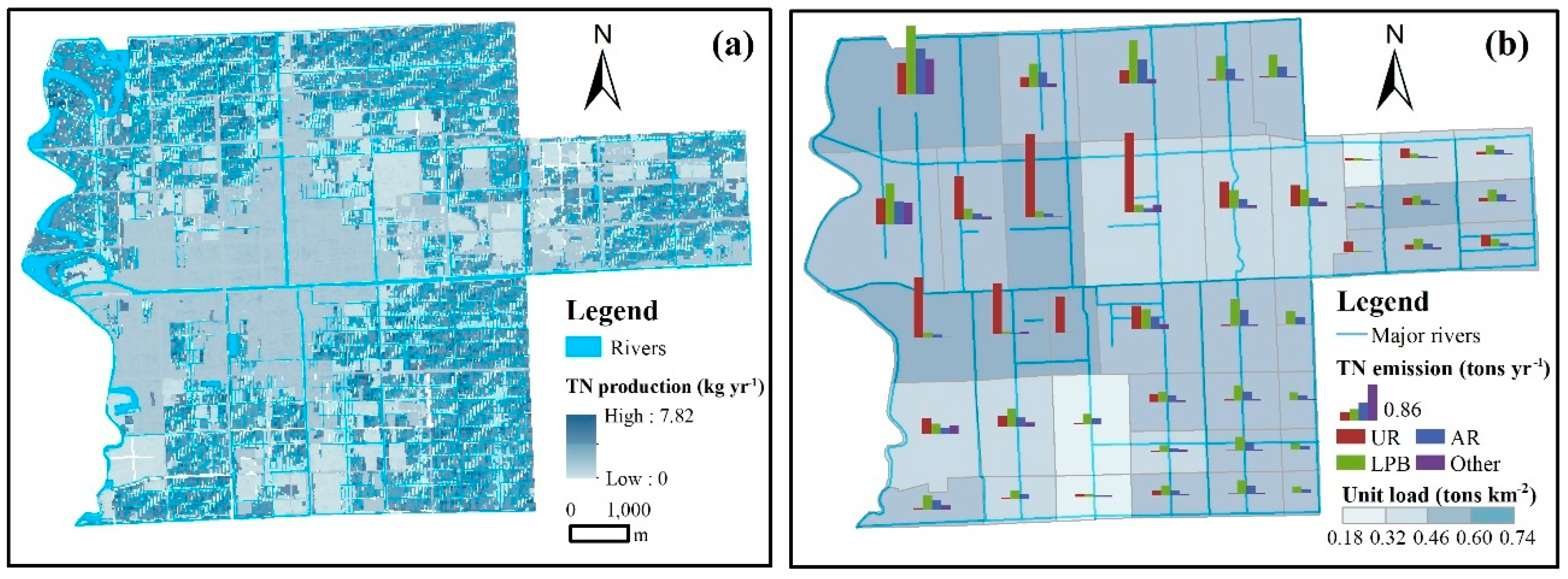
The annual average TN production per grid from the period 2000 to 2018 is shown in Figure 7a. The value ranged from 0 to 7.82 kg year⁻¹ for a 30 × 30 m grid—that is, 0–8.80 tons km⁻² year⁻¹. Ponds and farmlands (including irrigated lands, paddy field and orchards) had higher TN production intensities than other areas. The TN emissions from the four sources of pollution (UR, LPB, AR and other) for each sub-basin discharged into the river are shown in Figure 7b. The sub-basins with a high unit load being discharged into the river were located mainly in the north-western part of the study area. Among them, UR accounted for the largest proportion in most city-center sub-basins, and LPB had considerable impacts on some sub-basins in most suburban sub-basins.

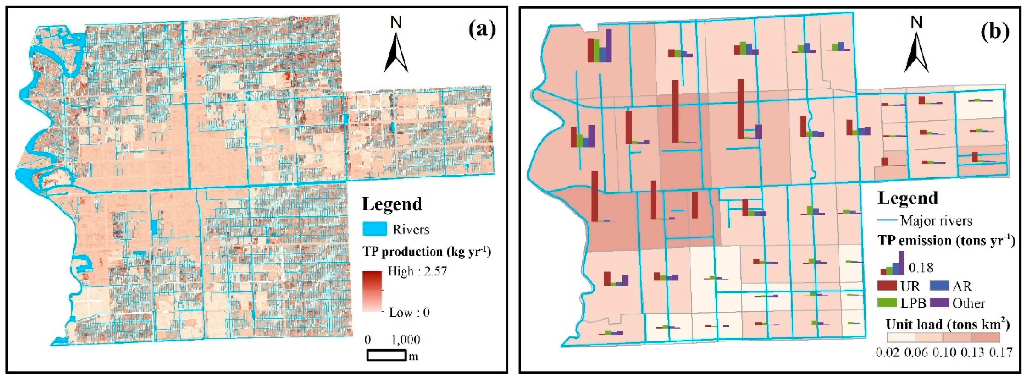
The NPS TP production per grid and emissions into the river each sub-basin are shown in Figure 8a,b. The TP production intensity was prominent in ponds and some farmland grids. The maximum value was 2.57 kg year⁻¹ for a 30 × 30 m grid—that is, 2.85 tons km⁻² year⁻¹. The total TP emissions and unit load for the north-western sub-basins were both higher than those of the other sub-basins. UR accounted for the largest proportion among these sub-basins. Aquaculture had relatively large impacts on sub-basins 2 and 7.

4.3. Temporal Variations in the Simulated NPS Loads

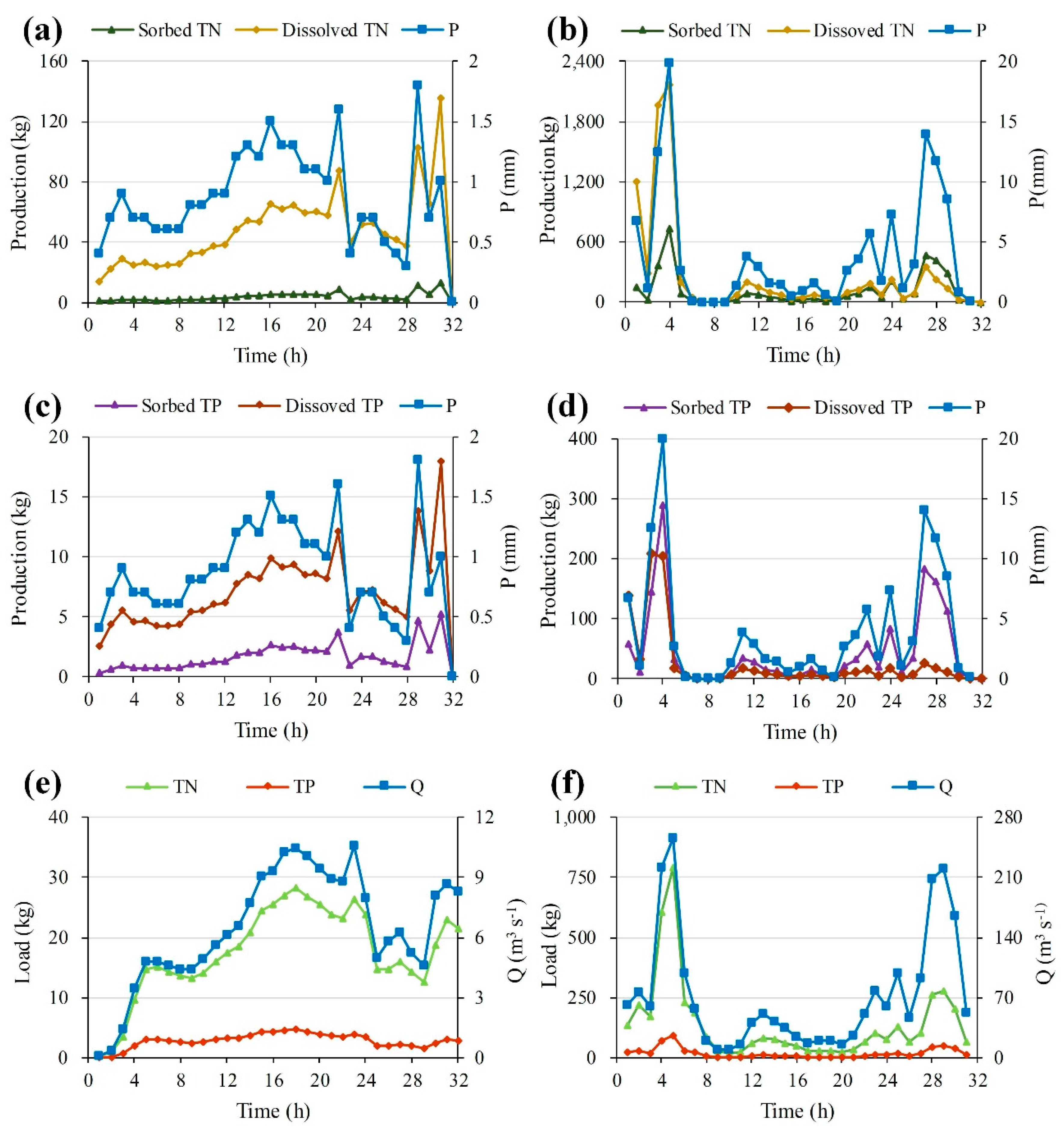
(1) NPS loads during rainfall events

Figure 9 shows the NPS TN and TP pollution loads resulting from two rainfall events. The sorbed and dissolved TN and TP were both consistent with the rainfall. The rainfall intensity in May was much greater than that in January. Dissolved nitrogen and phosphorus dominated when the rainfall intensity was low; as the rainfall intensity increased, the proportions of sorbed nitrogen and phosphorus increased, especially that of sorbed phosphorus.

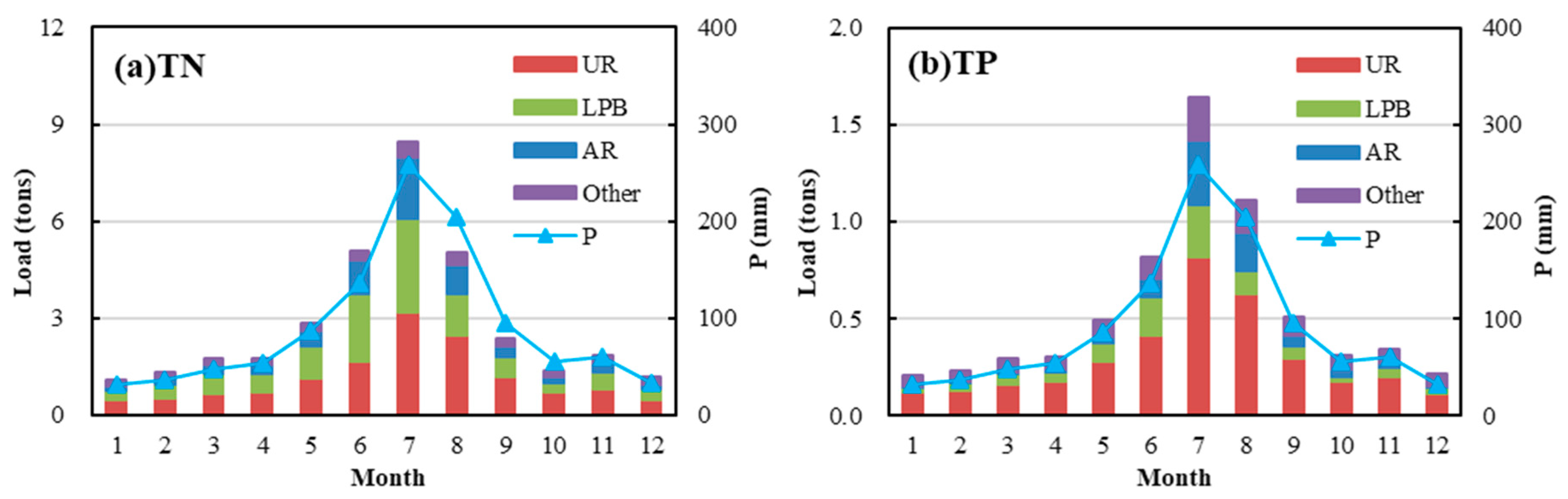
(2) Seasonal variation in NPS pollution

The NPS TN and TP loads into rivers displayed obvious differences on the monthly scale (Figure 10). High TN and TP emissions occurred mainly in summer (June, July and August), representing 56.2% and 58.0% of the total TN and TP loads, respectively, especially in July. Although there was more precipitation in August, the TN emissions were lower in August than in June. Overall, the relationship between TN emissions and rainfall was consistent with that between TP emissions and rainfall.

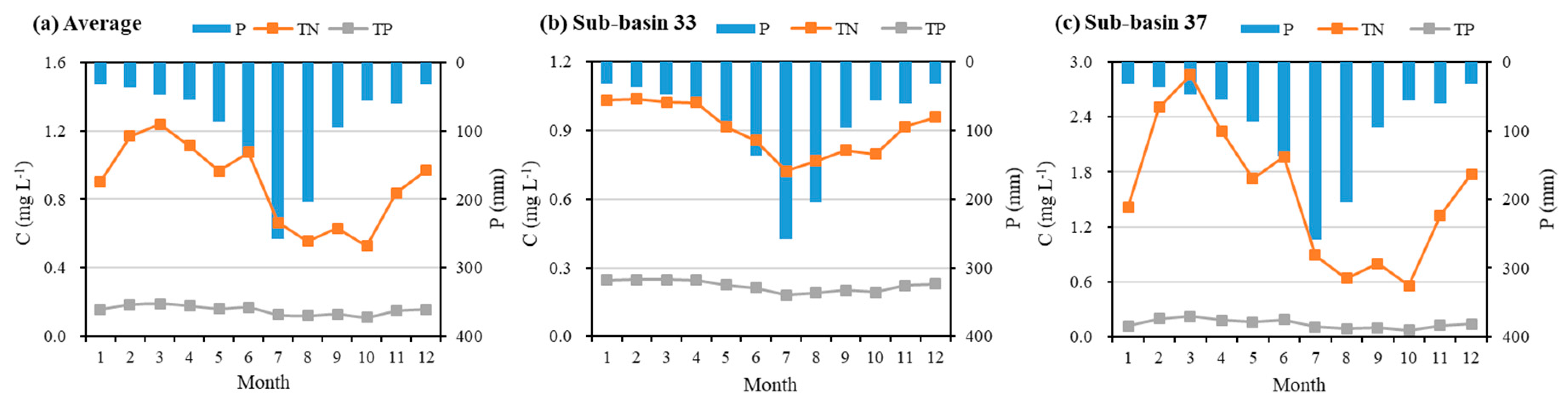
Figure 11 shows the monthly average concentrations of the NPS TN and TP emissions into rivers in each sub-basin without considering point and internal sources. The area-averaged concentrations of TN and TP were relatively low from July to October. The maximum concentrations of TN and TP were 1.24 mg L⁻¹ and 0.19 mg L⁻¹, respectively (Figure 11a). Sub-basins 33 and 37 represented the concentrations of typical urban area and farmland, respectively (Figure 11b,c). The monthly magnitude and its variation in the concentration of farmland were both higher than that of urban area. The typical farmland was characterized by a poorer water quality from February to April and a better water quality from July to October. This phenomenon was related to the pollution caused by livestock and poultry breeding in the farmland sub-basin.

(3) Interannual variation in NPS pollution

Based on the precipitation data from the period of 2000–2018, the NPS pollution emissions under different rainfall conditions in each year were calculated (Figure 12). The NPS TN and TP pollution emissions in the study area showed insignificant increasing trends. The minimum TN and TP pollution emissions occurred in 2001 (17.47 tons and 3.43 tons, respectively), while the maximum TN and TP pollution emissions occurred in 2015 (48.50 tons and 10.23 tons, respectively).

5. Discussion

5.1. Comparison with Other Studies

Water pollution has received widespread attention, and many studies have explored the spatial and temporal variations in sediment and pollutants.

Table 8. Some similar case studies in China with the simulated sediment and NPS pollution production per unit area (unit: tons km⁻² year⁻¹).

Case Study	Model	Sediment	TN	TP
Zhang et al. (2010, Binjiang watershed in Guangdong Province) [29]	Modified SWAT	-	0.693 (Watershed, farmland and other)	0.067 (Watershed, farmland and other)
Lin et al. (2010, watershed region of Meiliang Bay in the Yangtze River Delta) [30]	Integrated SEDD and PLOAD models	-	-	0.791~1.742 (Sub-basins, including arable, orchard, forest, grass, construction land and wetland)
Yang et al. (2003–2007, Songtao Reservoir on Hainan Island) [31]	EcoHAT (the Xinanjiang model coupled with SWAT)	31.29 (Forest); 32.6 (Grassland); 71.58 (Garden); 48.01 (Upland); 31.76 (Paddy)	0.334 (Forest); 0.32 (Grassland); 0.445 (Garden); 0.3711 (Upland); 0.389 (Paddy)	0.039 (Forest); 0.04 (Grassland); 0.048 (Garden); 0.047 (Upland); 0.044 (Paddy)
Huang et al. (2010, Sanjiang Plain in north-eastern China) [40]	SWAT	-	-	0.115 (Upland); 0.099 (Paddy); 0.056 (Forest); 0.049 (Wetland)
Wei et al. (1977–2013, the Sanjiang Plain of north-eastern China) [41]	SWAT	47.22 (Multi-year average)	0.792 (Multi-year average)	0.095 (Multi-year average)
Our results (2000–2018, our study area)	A combination of models	5.19 (Urban); 45.57 (Farmland); 5.17 (Other); 19.14 (Overall)	0.77 (Urban); 2.57 (Farmland); 0.23 (Other); 1.19 (Overall)	0.22 (Urban); 0.42 (Farmland); 0.07 (Other); 0.23 (Overall)

shows the simulation results of some of these studies from China. The simulated results of the sediment, TN and TP loads in our study area are comparable to the results reported in these case studies. In particular, the sediment load was above 30 tons km⁻² year⁻¹ in agricultural areas, e.g., the Sanjiang Plain, Hainan Island and our research area. However, there were some differences in the TN loads of different regions; nevertheless, the loads were generally greater than 0.3 tons km⁻² year⁻¹ in urban areas and agricultural areas. Additionally, the TP loads of different regions varied greatly; in some regions, the TP loads was as low as 0.04 tons km⁻² year⁻¹, while the TP load reached 1.7 tons km⁻² year⁻¹ in other regions.

5.2. Suggestions for Water Pollution Control

This study calculated various types of pollution loads. Among them, domestic pollution was the main source of pollutants, followed by NPS pollution. However, domestic pollution can be addressed by building pipe networks and corresponding sewage treatment plants. In contrast, NPS pollution is relatively difficult to control.

(1) Pollution load control priority

According to the simulation results of NPS pollution emissions, we prioritized the processing of pollution loads. The TN emission intensity decreased in the order of UR > LPB > AR > other, and the TP emission intensity decreased in the order UR > other > LPB > AR (Table 7 and Figure 10). Evidently, UR and LPB were the main sources of TN and TP emissions. Therefore, we should first consider reducing UR and LPB. To reduce the UR pollution load, it is fundamental to improve the urban ecological environment by increasing the urban greening rate and constructing sponge cities [42]. For LPB, the management strategy could be further optimized by returning waste to farmlands as much as possible, based on the pollution load carrying capacity of the land [43]. In addition, farmland strategies require improving the utilization rate of fertilizers [21] to reduce the pollution emissions. For aquaculture, some aquatic plants can be planted to absorb NPS pollutants [19].

The concentrations of NPS TN and TP in rivers were simulated (Figure 11). The concentrations of TN in sub-basin 37 exceeded the fourth category standard during the dry season, while that of TP below the same standard all year round (Figure 11c). The load reduction pressure of TN was greater than that of TP; hence, for farmlands, the focus should be on reducing TN. In addition, the concentrations of TN and TP emissions were relatively high during the dry season. Thus, the reduction of pollutants during the dry season should be of particular concern.

(2) Measures of water quality improvement

Measures to improve water quality mainly include reducing pollution emissions and diluting pollution loads. The water quality compliance requirements in the study area are fourth category—that is, TN < 1.5 mg L⁻¹ and TP < 0.3 mg L⁻¹. Based on the discharged pollutant loads in 2018, it is necessary to reduce TN by at least 193.54 tons and TP by at least 20.39 tons to meet these standards. If we adjust the supply water instead of reducing pollutants, at least 1.29 × 10⁸ m³ of pure water will need to be supplied to meet this standard. If the water used to dilute the pollutants satisfies the third category standard, it will be necessary to supply at least 3.87 × 10⁸ m³ of water. Among them, the amount of water needed to dilute NPS pollution with pure water or the third category standard water accounted for 16.9%. Certainly, this issue is serious and very common in the control of polluted rivers in many cities throughout China.

5.3. Uncertainties and Limitations

The study area is a man-made river basin, the boundaries of which are controlled by water conservancy engineering, and the river flow is controlled artificially. Unfortunately, only observation of the water level and not the flow volume are available. Therefore, a comparison of the simulated runoff with measured data cannot be provided. Here, as an alternative, we performed water balance analysis and the rationality analysis of the runoff coefficient to demonstrate the rationality of the simulation results. For such a rain-sewage confluence area, many sewage outlets lack measured (let alone continuously monitored) data, which makes it very difficult to verify the simulated results directly and therefore introduces some uncertainties. In this paper, an on-site investigation was conducted to mine available information, including the layout of sewage networks and their operation situations, the numbers of the overflow sewage outlets, and the discharges of industrial wastewater. The simulated NPS pollution results, in addition to the surveys of domestic pollution sources, online monitoring of industrial pollution sources, and laboratory tests of sediment contamination, were compared with the measured water quality. The simulated average concentration was consistent with the measured water quality. In addition, we compared the simulated results with those of the export coefficient model; their differences were less than 10% for the simulated total amount and for each component. Although it is impossible to provide further validation, these analyses still represent progress for a developing city with such a complex situation and limited data.

The four sources identified in this paper, namely UR, LPB, AR and other sources, were the four main NPS pollutants in the study area. The source data employed in this paper were obtained mainly from reference materials and local investigations, and some of these data were at monthly or annual scales. Although we considered the pollution load factors and made some adjustments for the pollution sources at different times, some uncertainties in the hourly and daily data remained. Of course, the temporal uncertainty in source data has certain impacts on hourly and daily simulated results but has little effect on monthly and annual-scale results. Therefore, the monthly and annual-scale simulation results are reliable.

Many parameters were involved in the model. Among them, the runoff generation module of the Xinanjiang model included 13 parameters (Table 3), which were mainly set based on the relevant literature. Some parameters significantly affected the water quantity simulation. During the parameter debugging process of the Xinanjiang model, we found that W₀, K and IMP were relatively sensitive. Table 4 shows several important parameters in the water quality simulation process. The vegetation cover and management factor and the maintenance measure factor were both key parameters for calculating the sediment and sorbed pollution production. Moreover, the ground wash coefficients of TN and TP (k_N and k_P) had considerable influences on the dissolved pollution load. Finally, the surface water treatment coefficients (FNS and FPS) and groundwater treatment coefficients (FNG and FPG) affected the total amounts of simulated NPS loads into rivers.

6. Conclusions

In this paper, a combination model was proposed and used to simulate the NPS TN and TP pollution load in the study area. We evaluated the spatiotemporal distribution of NPS pollution load. According to the results, we discovered the following:

(1) Ponds and farmlands had higher TN and TP production intensities than the other land use types, and the unit emissions in the northwestern region, which is mainly urban land and contains a great deal of aquaculture and LPB, were relatively higher;

(2) The variations in the monthly and interannual TN and TP loadings were consistent with the variations in rainfall. The emissions of TN and TP accounted for 56.2% and 58.0%, respectively, of the total in summer;

(3) NPS TN pollution was more serious than NPS TP pollution in the study area, especially in farmlands, and the concentrations of TN and TP emissions were relatively higher during the dry season;

(4) UR and LPB were the main sources of NPS TN and TP emissions in the study area. If NPS pollution cannot be removed from the study area, at least 2.19 × 10⁷ m³ of pure water or 6.56 × 10⁷ m³ of the third category standard water needs to be supplied to dilute the current rivers to meet the required fourth category standard.

References

- Zhang, K.; Wen, Z. Review and challenges of policies of environmental protection and sustainable development in China. J. Environ. Manag. 2008, 88, 1249–1261. [Google Scholar] [CrossRef] [PubMed]
- Chen, W.Y. Environmental externalities of urban river pollution and restoration: A hedonic analysis in Guangzhou (China). Landsc. Urban Plan. 2017, 157, 170–179. [Google Scholar] [CrossRef]
- Zhang, Q.H.; Yang, W.N.; Ngo, H.H.; Guo, W.S.; Jin, P.K.; Dzakpasu, M.; Yang, S.J.; Wang, Q.; Wang, X.C.; Ao, D. Current status of urban wastewater treatment plants in China. Environ. Int. 2016, 92–93, 11–22. [Google Scholar] [CrossRef] [PubMed]
- Xu, Z.; Xu, J.; Yin, H.; Jin, W.; Li, H.; He, Z. Urban river pollution control in developing countries. Nat. Sustain. 2019, 2, 158–160. [Google Scholar] [CrossRef]
- Han, D.; Currell, M.J.; Cao, G. Deep challenges for China’s war on water pollution. Environ. Pollut. 2016, 218, 1222–1233. [Google Scholar] [CrossRef] [PubMed] [Green Version]
- Zeng, F.; Cui, K.; Xie, Z.; Wu, L.; Liu, M.; Sun, G.; Lin, Y.; Luo, D.; Zeng, Z. Phthalate esters (PAEs): Emerging organic contaminants in agricultural soils in peri-urban areas around Guangzhou, China. Environ. Pollut. 2008, 156, 425–434. [Google Scholar] [CrossRef] [PubMed]
- Qin, H.; He, K.; Fu, G. Modeling middle and final flush effects of urban runoff pollution in an urbanizing catchment. J. Hydrol. 2016, 534, 638–647. [Google Scholar] [CrossRef]
- Qin, H.-P.; Khu, S.-T.; Yu, X.-Y. Spatial variations of storm runoff pollution and their correlation with land-use in a rapidly urbanizing catchment in China. Sci. Total Environ. 2010, 408, 4613–4623. [Google Scholar] [CrossRef]
- Mi, Y.; He, C.; Bian, H.; Cai, Y.; Sheng, L.; Ma, L. Ecological engineering restoration of a non-point source polluted river in Northern China. Ecol. Eng. 2015, 76, 142–150. [Google Scholar] [CrossRef]
- Shen, Z.; Zhong, Y.; Huang, Q.; Chen, L. Identifying non-point source priority management areas in watersheds with multiple functional zones. Water Res. 2015, 68, 563–571. [Google Scholar] [CrossRef]
- Zhang, B.; Cui, B.; Zhang, S.; Wu, Q.; Yao, L. Source apportionment of nitrogen and phosphorus from non-point source pollution in Nansi Lake Basin, China. Environ. Sci. Pollut. Res. 2018, 25, 19101–19113. [Google Scholar] [CrossRef] [PubMed]
- Wang, S.; He, Q.; Ai, H.; Wang, Z.; Zhang, Q. Pollutant concentrations and pollution loads in stormwater runoff from different land uses in Chongqing. J. Environ. Sci. 2013, 25, 502–510. [Google Scholar] [CrossRef]
- Ongley, E.D.; Xiaolan, Z.; Tao, Y. Current status of agricultural and rural non-point source Pollution assessment in China. Environ. Pollut. 2010, 158, 1159–1168. [Google Scholar] [CrossRef] [PubMed]
- Zheng, K.; Ni, F.; Deng, Y.; Wang, M. Study on the Non-point Source Pollution in the Mountainous Area of West Sichuan—A Case Study of Livestock and Poultry breeding in Baoxing County. IOP Conf. Ser. Earth Environ. Sci. 2019, 237, 022017. [Google Scholar] [CrossRef]
- Falconer, L.; Telfer, T.C.; Ross, L.G. Modelling seasonal nutrient inputs from non-point sources across large catchments of importance to aquaculture. Aquaculture 2018, 495, 682–692. [Google Scholar] [CrossRef] [Green Version]
- Li, C.; Zheng, X.; Zhao, F.; Wang, X.; Cai, Y.; Zhang, N. Effects of Urban Non-Point Source Pollution from Baoding City on Baiyangdian Lake, China. Water 2017, 9, 249. [Google Scholar] [CrossRef]
- Yang, X.; Liu, Q.; Fu, G.; He, Y.; Luo, X.; Zheng, Z. Spatiotemporal patterns and source attribution of nitrogen load in a river basin with complex pollution sources. Water Res. 2016, 94, 187–199. [Google Scholar] [CrossRef] [Green Version]
- Tu, M.-C.; Smith, P. Modeling Pollutant Buildup and Washoff Parameters for SWMM Based on Land Use in a Semiarid Urban Watershed. Water Air Soil Pollut. 2018, 229, 121. [Google Scholar] [CrossRef]
- He, Z.; Cheng, X.; Kyzas, G.Z.; Fu, J. Pharmaceuticals pollution of aquaculture and its management in China. J. Mol. Liq. 2016, 223, 781–789. [Google Scholar] [CrossRef]
- Zhou, P.; Huang, J.; Pontius, R.G.; Hong, H. New insight into the correlations between land use and water quality in a coastal watershed of China: Does point source pollution weaken it? Sci. Total Environ. 2016, 543, 591–600. [Google Scholar] [CrossRef]
- Hu, Y.; Cheng, H.; Tao, S. Environmental and human health challenges of industrial livestock and poultry farming in China and their mitigation. Environ. Int. 2017, 107, 111–130. [Google Scholar] [CrossRef] [PubMed]
- Ding, X.; Shen, Z.; Hong, Q.; Yang, Z.; Wu, X.; Liu, R. Development and test of the Export Coefficient Model in the Upper Reach of the Yangtze River. J. Hydrol. 2010, 383, 233–244. [Google Scholar] [CrossRef]
- Li, S.; Zhang, L.; Du, Y.; Liu, H.; Zhuang, Y.; Liu, S. Evaluating Phosphorus Loss for Watershed Management: Integrating a Weighting Scheme of Watershed Heterogeneity into Export Coefficient Model. Environ. Modeling Assess. 2016, 21, 657–668. [Google Scholar] [CrossRef]
- Shen, Z.; Liao, Q.; Hong, Q.; Gong, Y. An overview of research on agricultural non-point source pollution modelling in China. Sep. Purif. Technol. 2012, 84, 104–111. [Google Scholar] [CrossRef]
- Young, R.A.; Onstad, C.A.; Bosch, D.D.; Anderson, W.P. AGNPS: A nonpoint-source pollution model for evaluating agricultural watersheds. J. Soil Water Conserv. 1989, 44, 168–173. [Google Scholar]
- Lee, S.B.; Yoon, C.G.; Jung, K.W.; Hwang, H.S. Comparative evaluation of runoff and water quality using HSPF and SWMM. Water Sci. Technol. 2010, 62, 1401–1409. [Google Scholar] [CrossRef]
- Sisay, E.; Halefom, A.; Khare, D.; Singh, L.; Worku, T. Hydrological modelling of ungauged urban watershed using SWAT model. Modeling Earth Syst. Environ. 2017, 3, 693–702. [Google Scholar] [CrossRef]
- Tsihrintzis, V.A.; Hamid, R. Runoff quality prediction from small urban catchments using SWMM. Hydrol. Process. 1998, 12, 311–329. [Google Scholar] [CrossRef]
- Zhang, Z.; Huang, P.; Chen, Z.; Li, J. Evaluation of Distribution Properties of Non-Point Source Pollution in a Subtropical Monsoon Watershed by a Hydrological Model with a Modified Runoff Module. Water 2019, 11, 993. [Google Scholar] [CrossRef] [Green Version]
- Lin, C.; Wu, Z.; Ma, R.; Su, Z. Detection of sensitive soil properties related to non-point phosphorus pollution by integrated models of SEDD and PLOAD. Ecol. Indic. 2016, 60, 483–494. [Google Scholar] [CrossRef]
- Yang, S.; Dong, G.; Zheng, D.; Xiao, H.; Gao, Y.; Lang, Y. Coupling Xinanjiang model and SWAT to simulate agricultural non-point source pollution in Songtao watershed of Hainan, China. Ecol. Model. 2011, 222, 3701–3717. [Google Scholar] [CrossRef]
- Shangguan, W.; Dai, Y.; Liu, B.; Zhu, A.; Duan, Q.; Wu, L.; Ji, D.; Ye, A.; Yuan, H.; Zhang, Q.; et al. A China data set of soil properties for land surface modeling: China soil data set for land models. J. Adv. Modeling Earth Syst. 2013, 5, 212–224. [Google Scholar] [CrossRef]
- Ren-Jun, Z. The Xinanjiang model applied in China. J. Hydrol. 1992, 135, 371–381. [Google Scholar] [CrossRef]
- Yao, C.; Li, Z.; Yu, Z.; Zhang, K. A priori parameter estimates for a distributed, grid-based Xinanjiang model using geographically based information. J. Hydrol. 2012, 468–469, 47–62. [Google Scholar] [CrossRef]
- Fang, Y.-H.; Zhang, X.; Corbari, C.; Mancini, M.; Niu, G.-Y.; Zeng, W. Improving the Xin’anjiang hydrological model based on mass–energy balance. Hydrol. Earth Syst. Sci. 2017, 21, 3359–3375. [Google Scholar] [CrossRef] [Green Version]
- Muzik, I. Flood modelling with gis-derived distributed unit hydrographs. Hydrol. Process. 1996, 10, 1401–1409. [Google Scholar] [CrossRef]
- Kalyanapu, A.J. Effect of land use-based surface roughness on hydrologic model output. J. Spat. Hydrol. 2009, 9, 51–71. [Google Scholar]
- Wang, Y.; Yang, X. Sensitivity Analysis of the Surface Runoff Coefficient of HiPIMS in Simulating Flood Processes in a Large Basin. Water 2018, 10, 253. [Google Scholar] [CrossRef] [Green Version]
- Wang, P. Study and Application of Non-point Source Pollution Model of River Network Area Based on Digital Basin System. Doctoral Thesis, Hohai University, Nanjing, China, 2006. (In Chinese). [Google Scholar]
- Huang, H.; Ouyang, W.; Wu, H.; Liu, H.; Andrea, C. Long-term diffuse phosphorus pollution dynamics under the combined influence of land use and soil property variations. Sci. Total Environ. 2017, 579, 1894–1903. [Google Scholar] [CrossRef]
- Ouyang, W.; Jiao, W.; Li, X.; Giubilato, E.; Critto, A. Long-term agricultural non-point source pollution loading dynamics and correlation with outlet sediment geochemistry. J. Hydrol. 2016, 540, 379–385. [Google Scholar] [CrossRef]
- Xia, J.; Zhang, Y.; Xiong, L.; He, S.; Wang, L.; Yu, Z. Opportunities and challenges of the Sponge City construction related to urban water issues in China. Sci. China Earth Sci. 2017, 60, 652–658. [Google Scholar] [CrossRef]
- Foissy, D.; Vian, J.-F.; David, C. Managing nutrient in organic farming system: Reliance on livestock production for nutrient management of arable farmland. Org. Agric. 2013, 3, 183–199. [Google Scholar] [CrossRef]
Figure 1.
Location of the study area.
Figure 2.
Land use types in the study area.
Figure 3.
True-colour image with the distribution of sub-basins in the study area.
Figure 4.
Algorithm employed to simulate NPS pollutants.
Figure 5.
Annual average TN and TP concentrations observed in 2018.
Figure 6.
Annual average simulated results of the NPS pollution emissions into rivers from the combined model and the export coefficient model. TNm and TPm are the simulation results using the combined model, and TNe and TPe are the results using the export coefficient model.
Figure 7.
Annual average NPS TN load production per grid (a) and emissions into the river in each sub-basin (b).
Figure 8.
Annual average NPS TP load production per grid (a) and emissions into the river in each sub-basin (b).
Figure 9.
Pollution generation (a–d) and emission (e,f) processes for two rainfall events. (a,c,e) took place from 14:00 on January 3 to 21:00 on 4 January 2018. (b,d,f) took place from 12:00 on 5 May to 19:00 on 6 May 2018.
Figure 10.
Monthly average pollution emissions of each type of land use into rivers.
Figure 11.
Monthly average concentrations of the NPS TN and TP emissions into rivers during 2000–2018.
Figure 12.
Interannual pollution emissions of each source (UR, LPB, AR and other) into rivers.