Combined Use of Graphical and Statistical Approaches for Analyzing Historical Precipitation Changes in the Black Sea Region of Turkey

Abstract

Many statistical methods have been developed and used over time to analyze historical changes in hydrological time series, given the socioeconomic consequences of the changes in the water cycle components. The classical statistical methods, however, rely on many assumptions on the time series to be examined such as the normality, temporal and spatial independency and the constancy of the data distribution over time. When the assumptions are not fulfilled by the data, test results are not reliable. One way to relax these cumbersome assumptions and credibilize the results of statistical approaches is to make a combined use of graphical and statistical methods. To this end, two graphical methods of the refined cumulative sum of the difference between exceedance and non-exceedance counts of data points (CSD) and innovative trend analyses (ITA)-change boxes alongside the classical statistical Mann–Kendall (MK) method are used to analyze historical precipitation changes at 16 stations during 1960–2015 in the Black Sea region of Turkey. The results show a good match between the results of the graphical and statistical methods. The graphical CSD and ITA methods, however, are able to identify the hidden trends in the precipitation time series that cannot be detected using the statistical MK method.

1. Introduction

Precipitation is a vital hydro-climatic variable for assessing the availability of water resources which, in turn, brings about sustainable economic development of a country [1]. A decrease in precipitation can lead to a serious water shortage and drought and consequently to a decreased crop yield and food insecurity [2,3]. It is of a particular importance in semi-arid/arid developing countries due to the high dependence of their economy to rain-fed agriculture as well as their high sensitivity because of the climate conditions [4]. The sensitivity is even higher for the courtiers located in climatic transition areas such as the Mediterranean countries [5]. It is originated from the high spatiotemporal precipitation variabilities in the Mediterranean region [6] driven by a complex concurrent/lagged connections with climate teleconnections [7]. The region was also identified as a future climate change hotspot in terms of expected precipitation changes [4,7,8], although with a large projection uncertainty due to the meso-scale nature of precipitation [9].

On account of the remarkable consequences of precipitation changes, many scholars, in recent years, have been concerned about the changes in precipitation rate in response to global warming [10,11,12]. In this regard, analysis of temporal trends and shift change in historical precipitation series provides essential information for regional water resource planning and adaptation and mitigation strategies to climate changes [12,13]. To this end, various statistical methods have been developed and used over time. The classical methods, however, rely on many assumptions on the time series to be examined such as normality, temporal and special independency and the temporal constancy of the data distribution [14]. The Mann–Kendall (MK) test is well-known to be non-parametric and therefore not affected by the non-normality of data [15,16] and also because of its low sensitivity to abrupt breaks in inhomogeneous series [17]. The MK test has, therefore, gained popularity and numerous hydro-meteorological trend studies using this test have been carried out [18,19,20,21]. The problem with the popular non-parametric tests is that most of them tend to be purely statistical. Results of trend analyses which are purely statistical without graphical and exploratory data analyses can be meaningless in some cases [22]. In the same line, recently, Onyutha [23] showed that when graphical and statistical approaches are combined for trend analyses, they provide more supportive and influential information for inference than from the case when a non-parametric test is typically applied in a purely statistical way. Qualitative overall trends in time series by statistical approaches limit a representation of trends in sub-series [24], given the high sensitivity of these methods to the selection of the start and end years of the study period [25]. Furthermore, the use of an ensemble of graphical and statistical methods allows the uncertainty quantification of trend results due to the choice of a particular method, especially for the series characterized by long-term persistence [23].

To address the need of a visual quantitative trend analysis, several graphical methods have recently been developed such as the innovative trend analyses (ITA) [26] and the refined cumulative sum of the difference (CSD) test [27]. The CSD is a graphical-statistical approach based on the difference between exceedance and non-exceedance counts of data points [27]. The ITA method was further improved by the developer [28,29]. Some modified versions of the method were also proposed by other scholars such as double/triple ITA [30] and ITA-change boxes [31] for making it compatible with their research purposes and for a graphical comparison of the method’s results with the other trend methods [32]. Tabari et al. [33] suggested an improved version of the ITA for a decadal analysis where the time series in each decade is compared with that in the subsequent decade. Others have also applied the ITA to different portions of the time series [34,35,36].

This study encourages a combined use of graphical and statistical approaches rather than the use of individual methods as a stand-alone technique for analyzing historical time series. In this way, the results of different methods can be validated against each other, particularly considering the possible misunderstanding of the statistical significance concept [37]. The CSD, ITA-change boxes and MK methods are used to analyze historical precipitation changes during 1960–2015 in the Black Sea (BS) region of Turkey. The complex nature of rainfall in the region, which is influenced by different air masses and complex topographies, would better reveal the benefit of using combined graphical-statistical approach. The region is under the effect of polar air masses in winter and tropical air masses in summer. The orographic rainfall in the BS coastal region can be produced when air masses pick up moisture as they pass over the BS [38].

2. Materials and Methods

2.1. Study Area and Data

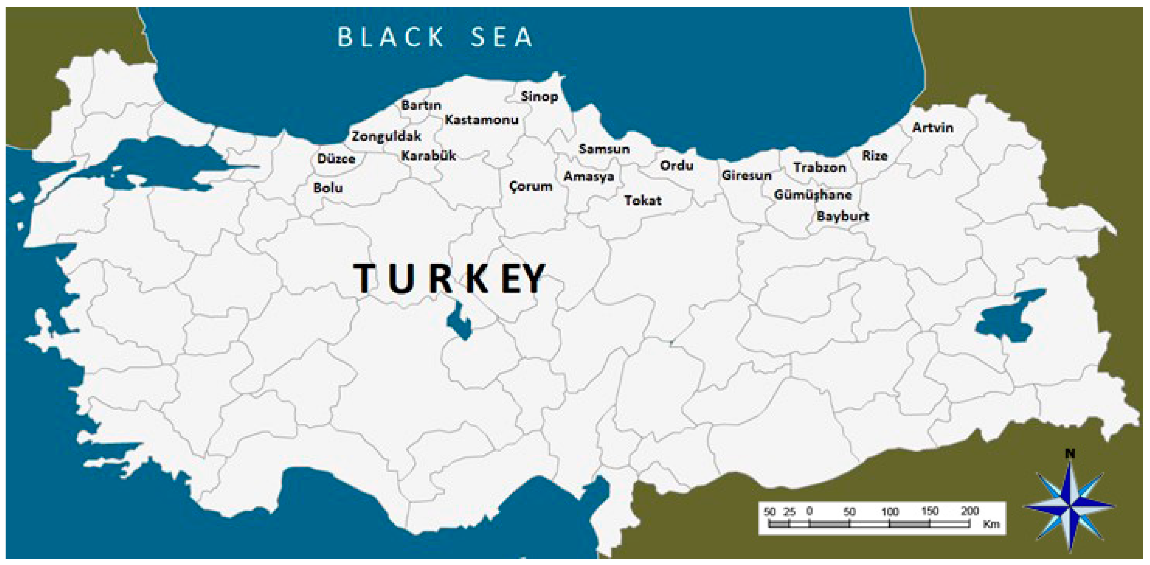
In the current study, monthly total rainfall data of 16 stations located in the BS region of Turkey were utilized. Figure 1 illustrates the location of stations and

Table 1. Statistical information of monthly rainfall data and the record length at the observation stations (X_min, X_max and X_mean: minimum, maximum and mean monthly precipitation; SD: standard deviation; C_v: coefficient of variation; C_sx: coefficient of skewness).

Station	Full Period	First Half	Second Half	Xmin	Xmax	Xmean	SD	Cv	Csx
Bartın	1965–2015	1964–1989	1990–2015	0	349.1	86.7	61.65	0.71	1.15
Zonguldak	1960–2015	1960–1987	1988–2015	0	359.8	101.3	68.6	0.68	0.86
Sinop	1960–2015	1960–1987	1988–2015	0	324.0	57.2	42.9	0.75	1.44
Samsun	1960–2015	1960–1987	1988–2015	0	350.3	58.8	40.4	0.69	1.68
Ordu	1963–2015	1963–1989	1990–2015	0.3	267.6	85.8	50.7	0.59	1.00
Giresun	1960–2015	1960–1987	1988–2015	0.2	521.6	104.97	61.89	0.59	1.41
Trabzon	1960–2015	1960–1983	1984–2005	2.8	293.0	68.1	43.8	0.64	1.28
Rize	1960–2015	1960–1987	1988–2015	8.2	516.6	186.4	102.1	0.55	0.84
Artvin	1960–2015	1960–1987	1988–2015	0.9	342.2	59.2	43.2	0.73	1.99
Bolu	1960–2015	1960–1987	1988–2015	0	174.4	46.4	29.1	0.63	0.94
Duzce	1960–2015	1961–1987	1988–2015	0	227.2	68.5	43.1	0.63	0.75
Kastamonu	1960–2015	1960–1987	1988–2015	0	278.7	41.6	31.7	0.76	1.80
Corum	1960–2015	1960–1987	1988–2015	0	220.1	36.8	28.4	0.77	1.37
Amasya	1960–2015	1960–1987	1988–2015	0	144.6	38.3	28.4	0.74	0.87
Tokat	1961–2015	1960–1987	1988–2015	0	141.1	36.1	27.3	0.76	0.87
Gumushane	1965–2015	1965–1989	1990–2015	0	141.9	38.5	26.8	0.70	0.78

sums up brief statistical characteristics of the used data for each station. The BS coast gets the highest precipitation in Turkey. The eastern BS is the only region in the country that receives precipitation throughout the year [39]. BS region has wet and humid climate (winter and summer have about 4 °C and 22 °C). Average annual total precipitation is 842 mm and 19.4% of this amount received in summer season. The region has very high relative humidity with the average annual value of 71% [40].

Turkey’s climate is affected by polar and tropical air masses in winter and summer, respectively. The continental polar is a cold and dry continental air mass which originates from Siberia, causing orographic rainfall. It is saturated while crossing the BS [41]. The air mass of marine polar originates from the Atlantic Ocean and goes across Europe and the Balkans. It unstably passes over Turkey and influences coastal areas’ rainfall (Black Sea), and snowfall occurs at higher elevations and in the interior [42,43]. The physiography of Turkey is highly effective on precipitation regimes. High relief and/or continentality have a high influence on rainfall deficit in interior regions; and, high orographic rains are observed (particularly in winter) where mountains are situated along the coast [43]. The chains of BS Mountain lay west to east along the coastline with about a 2000 m height and the highest point is 3973 m, and topography sharply changes from the coastline to inner region [44].

Rainfall data from 16 stations for the period 1960–2015 are used in this study. The data were divided into two equal parts before applying trend methods and each part and whole series were analyzed using implemented methods. Table 1 includes data periods and brief statistics of each station’s data. As clearly observed from the table that the east part of the BS region which includes Ordu, Giresun, Trabzon, Rize, and Artvin, generally has much more precipitation compared to other parts. Rize gets the highest precipitation while the lowest amount is received by Tokat and Corum. The rainfall data at the stations have a skewed distribution with a coefficient of variation of higher than 0.55.

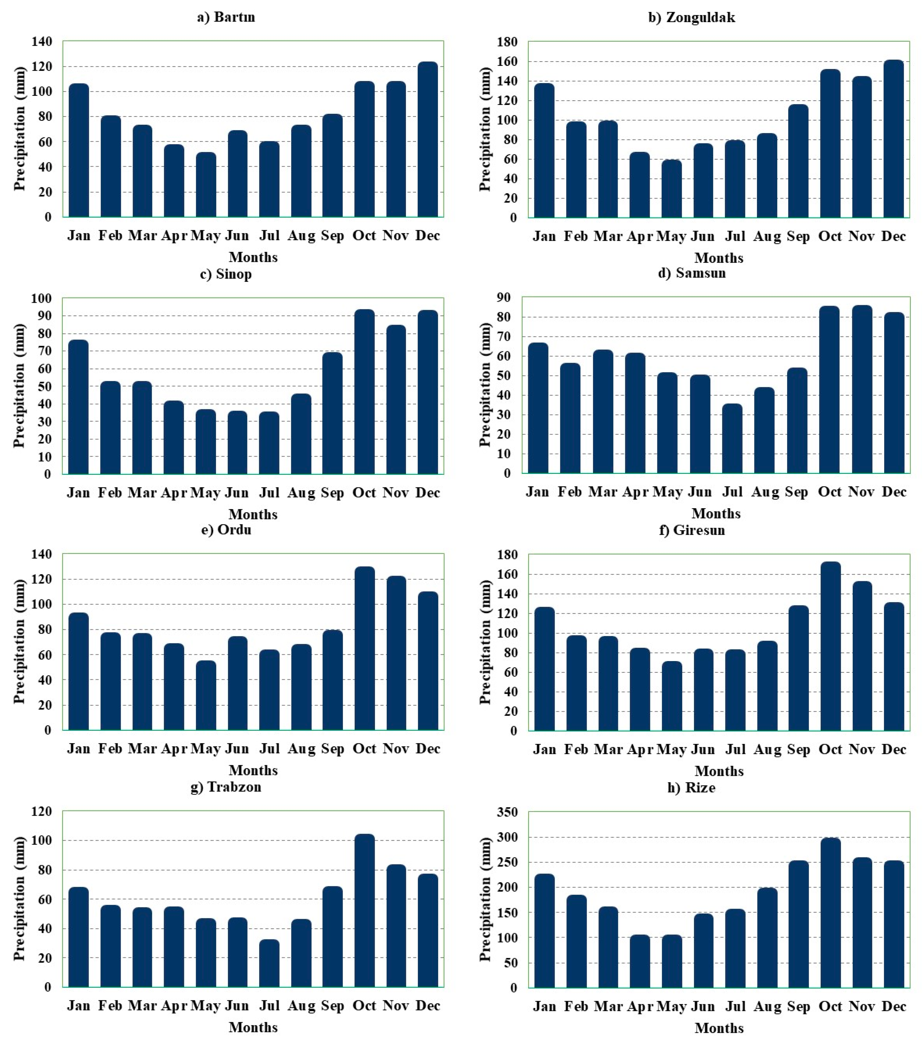
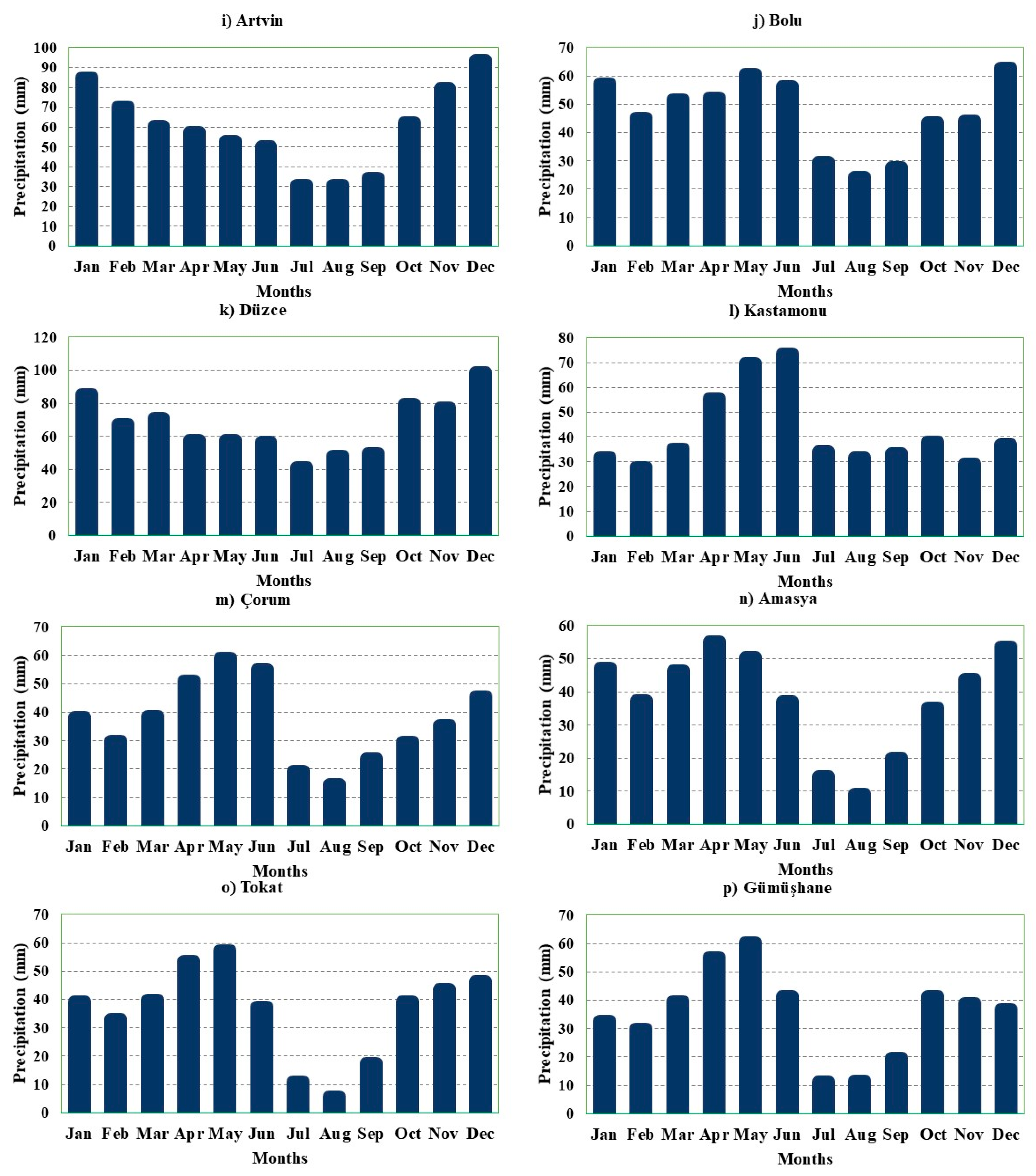
Histograms of monthly precipitation at each study station are illustrated in Figure 2. It is apparent from the figure that the distribution of the precipitation is similar through the year for the Bolu, Kastamonu, Corum, Amasya, Tokat and Gumushane where the minimum value is generally observed in August, while the maximum occurs in May. All these stations are situated in the inner part of the BS region. The coastal stations (Bartin, Zonguldak, Sinop, Samsun, Ordu, Giresun, Trabzon, Rize, Artvin and Duzce) generally have a similar precipitation distribution. Bartin, Zonguldak and Duzce located in the western BS region have the maximum precipitation in December, while the maximum shifts to October for Sinop, Samsun, Ordu, Giresun, Trabzon, Rize and Artvin situated in the middle and eastern BS region.

2.2. Methods

2.2.1. Refined Graphical–statistical CSD Trend Test and Diagnosis

The CSD-based approaches of trend analyses [27] comprise both graphical diagnosis and statistical test. If the given data of sample size n is represented by X such that Y is its replica, a transformed series (d) in terms of the exceedance and non-exceedance counts of data points can be obtained by [15,27]:

$$d_i=2{\displaystyle \sum _{j=1}^n{\mathrm{sgn}}_1\left(y_j-x_i\right)}-\left(n-{\displaystyle \sum _{j=1}^n{\mathrm{sgn}}_2\left(y_j-x_i\right)}\right) \mathrm{for} \mathrm{i} = 1, 2, \dots , n$$

(1)

where,

$${\mathrm{sgn}}_1\left(y_j-x_i\right)=\{\begin{array}{l}1\hspace{1em}\mathrm{if} \left(y_j-x_i\right)>0\\ 0\hspace{1em}\mathrm{if} \left(y_j-x_i\right)\le 0 \end{array}$$

(2)

$${\mathrm{sgn}}_2\left(y_j-x_i\right)=\{\begin{array}{l}1\hspace{1em}\mathrm{if} \left(y_j-x_i\right)=0\\ 0\hspace{1em}\mathrm{if} \left(y_j-x_i\right)<0 \mathrm{or} \left(y_j-x_i\right)>0\end{array}$$

(3)

We can obtain series (e₁) with the mean (variance) of zero (one) using

$$\gamma ={\displaystyle \sum _{i=1}^n{\left(d_i\right)}^2}$$

(4)

such that

$$e_i=d_i\times \sqrt{\frac{\left(n-1\right)}{\gamma }} \mathrm{for}\hspace{1em}1 \le i\le n$$

(5)

When a data point is tied n times, each value of d₁ becomes zero, meaning that e_i = 0 for 1 ≤ i ≤ n. A step-wise summation can be applied to d and e to obtain c and q, respectively, using

$$c_i={\displaystyle \sum _{j=1}^i{d}_j} \mathrm{for} 1 \le i \le n$$

(6)

$$q_k={\displaystyle \sum _{j=1}^k{e}_j} \mathrm{for} 1 \le k\le n$$

(7)

The trend statistic T_CSD can be given by

$$T_{CSD}={\displaystyle \sum _{j=1}^n{\displaystyle \sum _{i=1}^j{e}_i}}$$

(8)

The distribution of T_CSD is approximately normal with the mean of zero and the variance given by

$$V=\frac{n(n^2-1)}{12}$$

(9)

The statistic Z_CSD with the mean of zero and variance equal to one can be computed using

$$Z_{CSD}=\frac{T_{CSD}}{\sqrt{V*}}$$

(10)

where $V*=\lambda \times V^{\mathsf{\Omega }}$, while $\lambda =-2.99152H^2+3.08938H+0.31343$, $\mathsf{\Omega }=0.33419H^2+0.16046H^2+0.82744$ and H denotes the Hurst exponent. Let Z_α/2 denote the standard normal variate at a selected α. The null hypothesis H₀ (no trend) is rejected if |Z| > Z_α/2 at α; otherwise, the H₀ is not rejected.

To perform graphical diagnoses of the changes in the series, c can be plotted against the time (e.g., year) of observation to obtain the CSD-plot. In the CSD-plot, the c = 0 line becomes the reference typifying the case with completely no trend or when all the data points are tied up. If the data have a positive (negative) trend, the scatter points in the CSD-plot will tend to form a curve most of which falls above (below) the reference. If there is no trend in the data, the scatter points cross the reference randomly in the CSD-plot.

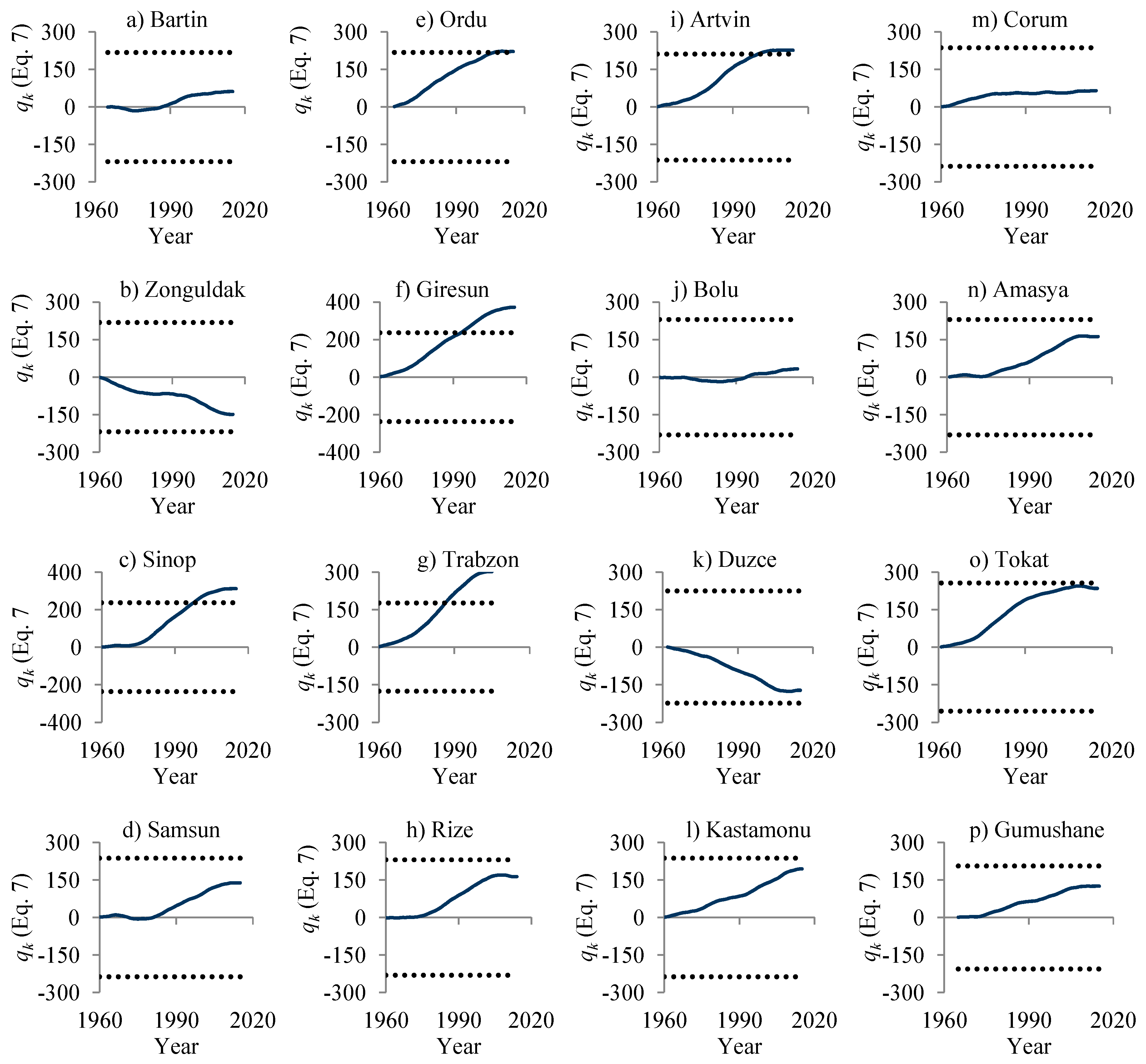
Further graphical diagnosis to confirm trend the direction can be performed through the plot of q_k versus k or time of observations. Positive and negative trends are shown by the right tail of the scatter plot above and below the reference (q_k = 0 line), respectively. At a selected α, (100–α)% Confidences Interval (CI) limits are constructed and included in the plot of q_k versus k. The (100–α)% CI limits Q based on the V* and Z_α/2 given by

$$Q=\pm Z_{\alpha /2}\times \sqrt{V*}$$

(11)

where V* is as defined from Equation (10). If any scatter points fall outside the (100–α)% CI limits, the H₀ (no trend) is rejected, otherwise, the H₀ is not rejected [27].

2.2.2. Mann–Kendall (MK) Test

The MK test [45,46] is calculated as follows:

The test statistic S is first calculated based on the sign function $\mathrm{sgn}(\theta )$:

$$S={\displaystyle \sum }_{i=1}^{n-1} {\displaystyle \sum }_{j=i+1}^n\mathrm{sgn} \left(x_j-x_i\right)$$

(12)

where x_j and x_i are the sequential data values, n is the length of the data set and $\mathrm{sgn}(\theta )$ is equal to 1, 0, −1 if θ is greater than, equal to, or less than zero, respectively. The variance of S is obtained through:

$$\mathrm{Var} \left(S\right) = \frac{n \left(n-1\right) \left(2n+5\right)-{\displaystyle {\displaystyle \sum }_{i=1}^m} t_i \left(t_i-1\right) \left(2t_i+5\right)}{18}$$

(13)

where m is the number of tied groups (a tied group is a set of sample data having the same value) and t_i is the number of data points in the ith group. Finally, the Mann–Kendall statistic, Z_MK, is given by:

$$Z_{MK}= \{\begin{array}{ccc} \frac{S - 1}{\sqrt{\mathrm{Var} (S)}}& \mathrm{if}& S >0\\ 0& \mathrm{if}& S= 0\\ \frac{S + 1}{\sqrt{\mathrm{Var} (S)}}& \mathrm{if}& S < 0\end{array}$$

(14)

As the Z_MK values are approximately normally distributed, the null hypothesis, H₀, of no trend is rejected if $\left|Z_{MK}\right|>\left|Z_{\alpha /2}\right|$, where Z_MK is taken from the standard normal distribution table and α is the significance level. The positive and negative values of Z_MK denote increasing and decreasing trends, respectively.

2.2.3. ITA and Change Boxes

Based on quantile-quantile plots (Q-Q plots), Şen [26] proposed a method for investigating changes in time series. In this method, quantiles, arranged data in either descending or ascending order, in the first and second halves of the time series are plotted as scatter points on the X- and Y-axis respectively and compared against the 1:1 (45°) straight line. The scatter points within the upper and lower triangles of the square area represent increasing and decreasing trends, respectively. There is no trend in the time series if the data more or less parallel with the 1:1 line. In the case of a nonmonotonic trend in time series, the trends in high, medium and low values are analyzed separately. Separation of data into these three groups can be done either in a subjective (depending on the study purpose) or objective manner. In the latter, the ranges of the three groups are determined as:

$$X_{low} => X<\overline{X}-{\sigma }_X$$

(15a)

$$X_{mediun} => \overline{X}-{\sigma }_X< X<\overline{X}+{\sigma }_X$$

(15b)

$$X_{high} => X>\overline{X}+{\sigma }_X$$

(15c)

where $\overline{X}$ are ${\sigma }_X$ the mean and standard deviation of the first half-time series.

Alashan [30] added change boxes to the ITA method to numerically otain changes for each group. The changes are calculated as a ratio of quantiles in the second half over those in the first half. The ranges of change are plotted as change boxes for each group.

2.2.4. Trend Magnitude

The magnitude of trend m in each series was computed using [47,48]

$$m=\mathrm{Median} (\frac{x_j-x_i}{j-i}) \mathrm{for} \mathrm{all} i<j$$

(16)

where x_j and x_i are the jth and ith observations, respectively.

3. Results and Discussion

Table 2. Statistical results of trend analysis for seasonal and annual rainfall using the CSD method.

Rainfall Station	Full Time Series					First Half Sub−series					Second Half Sub−series
	Win	Spr	Sum	Aut	Ann	Win	Spr	Sum	Aut	Ann	Win	Spr	Sum	Aut	Ann
Bartin	−0.63	−0.48	0.20	0.26	0.57	−1.69	−2.44	0.68	0.21	−0.83	1.58	1.64	−0.84	2.88	0.03
Zonguldak	−0.61	−1.14	−1.31	−0.43	−1.22	−1.65	−1.66	−0.01	−0.11	−1.89	2.58	1.41	−1.64	2.77	−1.99
Sinop	0.62	0.51	0.98	0.14	2.11	−2.32	−1.38	0.65	−2.16	−1.52	1.48	0.67	0.40	−0.38	0.36
Samsun	−0.06	−0.19	1.22	0.04	0.97	−1.92	−0.42	1.01	−2.28	−1.00	1.59	0.84	0.79	1.71	0.86
Ordu	0.63	1.92	−0.74	1.25	1.88	0.45	1.76	0.08	1.40	1.93	−0.75	−0.31	1.37	0.20	0.92
Giresun	−0.26	0.73	0.53	0.19	3.08	0.00	0.23	1.21	−0.31	1.68	1.35	0.01	−0.36	0.66	1.36
Trabzon	1.93	1.53	1.64	1.58	3.35	0.15	−0.99	0.64	−0.36	−0.09	1.53	2.01	0.33	0.32	1.99
Rize	−0.29	−1.16	1.35	−0.70	1.75	−0.04	−2.24	−0.43	−0.37	−0.64	−0.81	0.41	1.37	−0.92	0.47
Artvin	0.30	1.51	1.47	0.70	2.64	1.15	0.07	−1.31	1.17	0.21	−2.16	1.21	0.86	−2.39	−0.76
Bolu	−0.98	0.72	0.39	0.07	0.32	0.24	−1.58	−0.16	1.22	−0.69	1.52	1.94	0.12	1.99	1.31
Duzce	−1.15	−1.33	−0.71	−0.87	−1.61	−0.87	−0.93	0.60	0.20	−0.31	−0.48	0.18	−0.71	0.75	−0.83
Kastamonu	0.01	1.36	0.94	−0.47	1.40	0.33	1.19	0.16	0.37	0.96	1.31	0.91	1.39	2.19	1.82
Corum	−1.32	0.29	1.13	−0.38	0.79	−0.20	1.12	−0.28	0.56	1.00	0.86	−1.05	−0.21	2.49	−0.19
Amasya	−0.99	1.10	2.11	−0.73	1.22	−2.02	−0.43	1.59	−0.46	0.35	1.86	0.37	1.60	3.11	1.94
Tokat	−1.21	1.33	0.89	−0.06	1.80	−0.81	1.15	0.51	1.23	1.60	0.42	−1.13	0.44	2.48	−0.62
Gumushane	−0.91	0.41	−0.25	1.36	0.99	0.09	−0.41	0.11	1.15	1.03	1.01	0.36	−0.62	2.90	0.90

The results in this table are for Annual (Ann) series as well as those of winter (Win), Spring (Spr), summer (Sum), and Autumn (Aut) seasons. Results for which the H₀ (no trend) was rejected (p < 0.05) are presented in bold.

shows trend results for annual rainfall. The corresponding trend magnitudes are presented in

Table 3. The magnitude (mm/year) of the linear trends in annual rainfall.

Rainfall Station	Full Time Series					First Half Sub−series					Second Half Sub−series
	Win	Spr	Sum	Aut	Ann	Win	Spr	Sum	Aut	Ann	Win	Spr	Sum	Aut	Ann
Bartin	−0.71	−0.35	0.19	0.29	0.95	−4.6	−3.54	1.28	0.82	−4.95	3.19	2.14	−1.84	6.47	−0.72
Zonguldak	−0.51	−0.63	−0.97	−0.43	−1.45	−2.3	−3.46	−0.05	−0.01	−6.77	6.06	1.31	−3.26	6.62	−6.78
Sinop	0.40	0.24	0.51	0.09	2.46	−3	−1.52	0.97	−2.20	−6.22	1.55	0.79	0.67	−0.42	0.78
Samsun	0.04	−0.05	1.21	0.01	1.20	−2.8	−0.55	1.24	−3.39	−3.65	2.46	0.79	1.43	1.92	2.61
Ordu	0.33	0.88	−0.54	1.16	2.22	0.6	1.52	−0.10	2.44	9.24	−0.9	−0.51	2.68	0.49	1.33
Giresun	−0.18	0.41	0.36	0.15	3.44	−0	0.59	1.34	−0.42	3.94	1.76	0.26	−1.59	1.31	5.86
Trabzon	1.33	0.60	0.68	1.34	4.32	0.63	−0.93	0.89	−0.58	−0.09	2.7	2.77	0.24	1.24	6.61
Rize	−0.53	−0.81	1.07	−0.92	3.94	−0.5	−3.07	−1.24	−0.64	−4.15	−2.1	0.37	5.12	−1.82	3.21
Artvin	0.13	0.35	0.64	0.49	2.23	2.35	0.01	−0.71	1.80	0.58	−5.8	1.00	0.95	−8.19	−2.55
Bolu	−0.14	0.21	0.38	0.06	0.39	0.03	−1.54	−0.13	1.68	−0.92	1.85	2.19	0.16	2.83	2.36
Duzce	−1.28	−0.37	−0.39	−0.71	−1.85	−1.4	−1.58	0.83	0.50	−1.32	−1.3	0.47	−2.26	1.17	−1.84
Kastamonu	−0.04	0.49	0.56	−0.17	1.39	0.41	1.36	0.01	0.43	2.16	1.21	1.39	2.92	1.88	5.40
Corum	−0.59	0.06	0.30	−0.13	0.30	−0.2	0.94	−0.52	0.99	1.88	1.33	−0.91	−0.59	2.77	−0.71
Amasya	−0.80	0.33	0.37	−0.53	0.83	−2.6	−0.51	1.27	−0.59	0.71	2.96	0.73	1.12	3.90	4.26
Tokat	−0.53	0.43	0.28	0.02	1.27	−0.9	0.82	0.24	1.88	3.34	0.24	−0.96	0.28	1.89	−1.25
Gumushane	−0.29	0.20	−0.03	0.50	0.87	0.07	−0.52	0.15	1.13	2.62	1.12	0.71	−0.32	2.26	1.94

The results in this table are for Annual (Ann) series as well as those of winter (Win), Spring (Spr), summer (Sum), and Autumn (Aut) seasons.

. Considering the full time series, the H₀ (no trend) was not rejected (p > 0.05) in the Winter, Spring and Autumn rainfall at all the selected stations. However, the H₀ (no trend) was rejected (p < 0.05) in the Summer rainfall from Amasya station. The annual rainfall was mainly characterized by positive trends for which H₀ (no trend) was rejected (p < 0.05) in the rainfall from 4 stations including Sinop, Giresun, Trabzon and Artvin. Considering the trends in the first and second halve of the time series, the highest number of significant trends is observed in the Autumn rainfall of the second half sub-series with significant trends at 56% of the selected stations.

Regardless of the significance of the trends, the winter and spring seasons from the first (second) half of the data period were characterized mainly by a decrease (an increase) in rainfall. The direction (and/or significance) of the trends varied among various seasons. In other words, by considering the same period, it is noticeable that rainfall of some seasons experienced a decrease while series from other seasons exhibited an increase. This indicates the difference in variability of rainfall among seasons. This also suggests that the drivers of rainfall variability may also vary among the seasons. It can be noted that the trend directions and magnitude from the annual time scale comprise the net effects of the negative and positive trends from the various seasons.

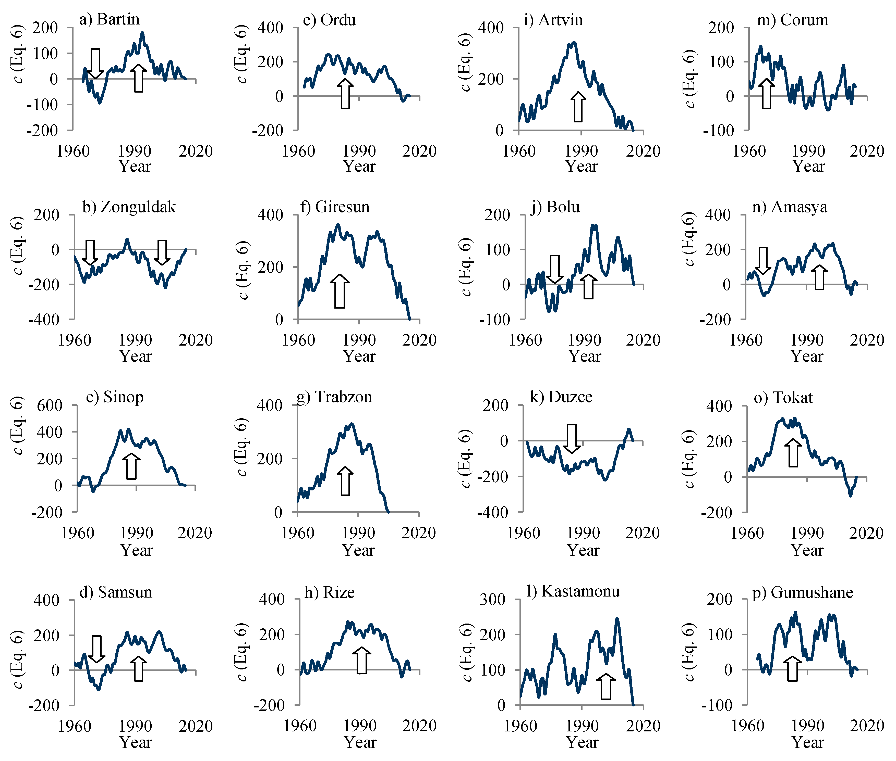
Figure 3, as the CSD-plot, shows the cumulative effects of temporal variations in annual rainfall. The upward/downward arrows in Figure 3a–p show positive/negative sub-trends. The horizontal line for c = 0 is taken as the reference. It is evident that the scatter points in the CSD plot formed a curve above the reference for a number of stations (see Figure 3c–i,l,n–p). It means that at these stations, the changes in annual rainfall were mainly dominated by monotonic increase over the full data period. This finding is in line with the results of the statistical CSD test (see Table 2). At some stations (see Figure 3a,d,j,n), the scatter points formed small curves above and below the reference. This meant that for these stations both positive and negative sub-trends existed in the annual rainfall data. At Zonguldak (Figure 3b), there were two negative sub-trends (over the periods 1960–1986 and 1987–2015).

What cannot escape a quick notice is that the lengths of the sub-trends tended to vary from one station to another something which can be thought of in terms of the spatial variation in rainfall characteristics. An important note to be taken in that the statistical results in Table 2 and Table 3 were obtained on the assumption that sub-trends exist over the entire first and second halves of the data. However, the CSD-plots (Figure 3) clearly show that sub-periods with increasing and decreasing sub-trends can occur over unknown times of the data period (not necessarily first and second halves). Figure 4 shows results of graphically detected significance of the trends in annual rainfall across the study area. Rainfall at Zonguldak and Duzce (Figure 4b,k) exhibited a decrease. However, the remaining stations showed increase in rainfall (Figure 4a,c–j,l–p). The H₀ (no trend) was rejected in terms of rainfall at Sinop, Giresun, Trabzon, and Artvin (Figure 4c,f–g,i).

Table 4. Statistical results (Z_MK) of trend analysis for annual rainfall using the MK method.

Rainfall Station	Full Time Series					First Half Sub−series					Second Half Sub−series
	Win	Spr	Sum	Aut	Ann	Win	Spr	Sum	Aut	Ann	Win	Spr	Sum	Aut	Ann
Bartin	−0.26	−0.49	0.26	0.32	0.50	−0.63	−2.31	0.63	0.30	−1.17	1.76	1.45	−0.66	2.71	−0.49
Zonguldak	−0.73	−0.94	−1.38	−0.76	−1.16	−1.63	−1.72	−0.02	0.02	−1.92	2.70	1.52	−1.52	2.53	−1.70
Sinop	0.78	0.62	1.11	−0.11	2.18	−2.75	−1.32	0.77	−1.80	−1.88	1.18	0.85	0.49	−0.86	0.38
Samsun	0.09	−0.11	2.36	−0.17	1.32	−2.23	−0.49	1.01	−2.43	−1.01	1.32	0.85	1.02	1.22	1.05
Ordu	0.96	1.84	−0.77	1.10	2.11	1.04	0.88	−0.04	1.28	1.97	−0.66	−0.93	1.42	0.29	0.48
Giresun	−0.31	0.70	0.48	0.19	3.28	−0.54	0.24	0.97	−0.10	1.68	0.29	0.04	−0.45	0.53	1.48
Trabzon	1.35	1.40	1.58	1.18	3.39	0.21	−1.00	0.58	−0.32	−0.05	0.74	2.17	0.24	−0.03	2.01
Rize	−0.46	−1.34	1.19	−1.02	1.77	−0.36	−2.23	−0.53	−0.26	−0.57	−1.44	0.22	1.26	−1.18	0.55
Artvin	0.12	1.35	1.93	0.97	2.25	0.79	0.02	−1.13	1.28	0.30	−2.31	1.09	0.85	−2.23	−0.69
Bolu	−0.48	0.63	0.72	−0.12	0.56	0.19	−1.42	−0.10	1.40	−0.61	1.52	1.76	0.13	1.50	1.05
Duzce	−1.66	−0.78	−0.66	−1.08	−1.54	−0.13	−0.79	0.64	0.52	−0.33	−0.17	0.25	−0.79	0.51	−0.83
Kastamonu	−0.12	0.98	0.85	−0.75	1.58	0.42	1.17	0.02	0.40	1.01	1.05	0.77	1.40	1.96	1.92
Corum	−1.32	0.19	0.58	−0.69	0.41	−0.34	1.21	−0.28	0.69	1.03	0.38	−1.15	−0.26	2.13	−0.38
Amasya	−1.26	0.86	1.61	−1.39	1.36	−1.42	−0.38	1.06	−0.46	0.30	1.80	0.71	1.03	1.93	2.04
Tokat	−0.88	1.13	0.99	−0.33	2.03	−0.21	0.96	0.13	1.04	1.63	0.22	−0.87	0.18	1.37	−0.54
Gumushane	−0.43	0.39	−0.13	1.60	1.19	0.53	−0.44	0.12	1.23	1.48	1.05	0.48	−0.49	2.27	1.19

The results in this table are for Annual (Ann) series as well as those of winter (Win), Spring (Spr), summer (Sum), and Autumn (Aut) seasons. Bold values of Z_MK denote that the H₀ (no trend) was rejected at the 5% significance level.

illustrates the MK trend test results of annual rainfall and bold values of Z_MK denote that the H₀ (no trend) was rejected at the 5% significance level. As observed from the table, there are significant increasing trends for the annual rainfall of Sinop, Ordu, Giresun, Trabzon, Artvin and Tokat, while seasons do not have significant trend when full rainfall time series is considered. Only summer season of Samsun has an increasing trend with respect to 5% significance level. Considering the first and second half of the time series, it is observed that most of the annual trends disappeared; there is only one station, Ordu, with increasing trend in the first half while two stations, Trabzon and Amasya have significantly increasing trends in the second half of the annual rainfall series. In this case, however, seasonal trends increased; Winter rainfall of Sinop and Samsun, Spring rainfall of Bartin and Rize and Autumn rainfall of Samsun have decreasing trends in the first halve while in the second sub series, Winter rainfall of Zonguldak and Artvin, Spring rainfall of Trabzon, and Autumn rainfall of Bartin, Zonguldak, Artvin, Kastamonu, Corum and Gumushane have increasing/decreasing trends. Summer rainfall does not show significant trend in subseries (first and second halves).

Table 5. Trends and change rates of annual rainfall at all stations using the ITA-CB (Minimum, mean and maximum percentage changes for each group are presented).

Station	Low Group			High Group			All Group
	Min	Mean	Max	Min	Mean	Max	Min	Mean	Max
Bartin	4.25	6.09	7.50	−0.88	6.75	11.90	−0.88	6.65	11.90
Zonguldak	−8.04	4.29	13.39	5.12	15.27	3.27	13.39	3.27	20.00
Sinop	35.17	46.70	59.29	−3.49	4.15	10.24	59.29	19.25	59.29
Samsun	14.42	17.70	21.54	−6.33	−4.05	−1.29	−6.33	6.52	21.54
Ordu	16.69	18.00	20.69	−3.90	−1.04	3.22	−3.90	6.06	20.69
Giresun	−8.18	1.61	5.08	3.48	13.01	22.42	−8.18	7.58	22.42
Trabzon	9.72	16.69	19.46	10.52	12.27	13.60	6.43	13.70	19.46
Rize	−35.57	13.40	4.82	3.65	3.93	21.12	−35.57	7.23	21.12
Artvin	18.81	21.29	27.23	3.86	8.96	15.09	3.86	15.09	27.23
Bolu	−6.57	−3.43	1.35	−4.80	1.54	5.26	−6.57	0.98	6.15
Duzce	−11.81	−1.54	3.68	−9.72	−5.38	3.06	−11.81	−5.20	3.68
Kastamonu	−6.83	−2.22	8.91	2.80	20.10	5.95	−6.83	5.95	40.51
Corum	−21.80	4.81	17.53	4.47	6.69	8.29	−21.80	1.75	17.53
Amasya	−1.60	1.68	7.73	−4.00	4.56	2.29	−4.00	2.29	11.15
Tokat	6.64	9.61	13.08	5.33	6.64	8.18	13.09	8.18	13.09
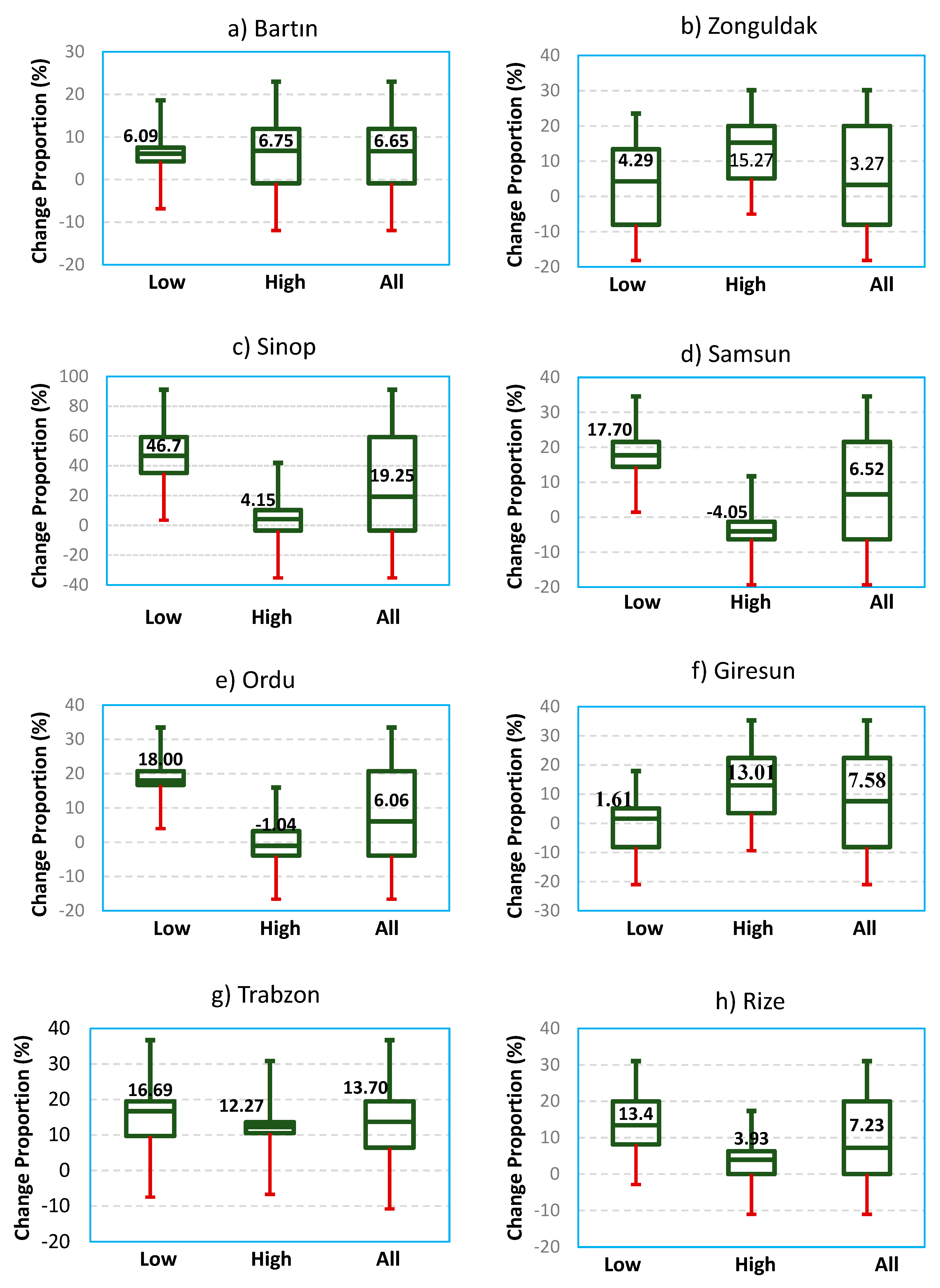
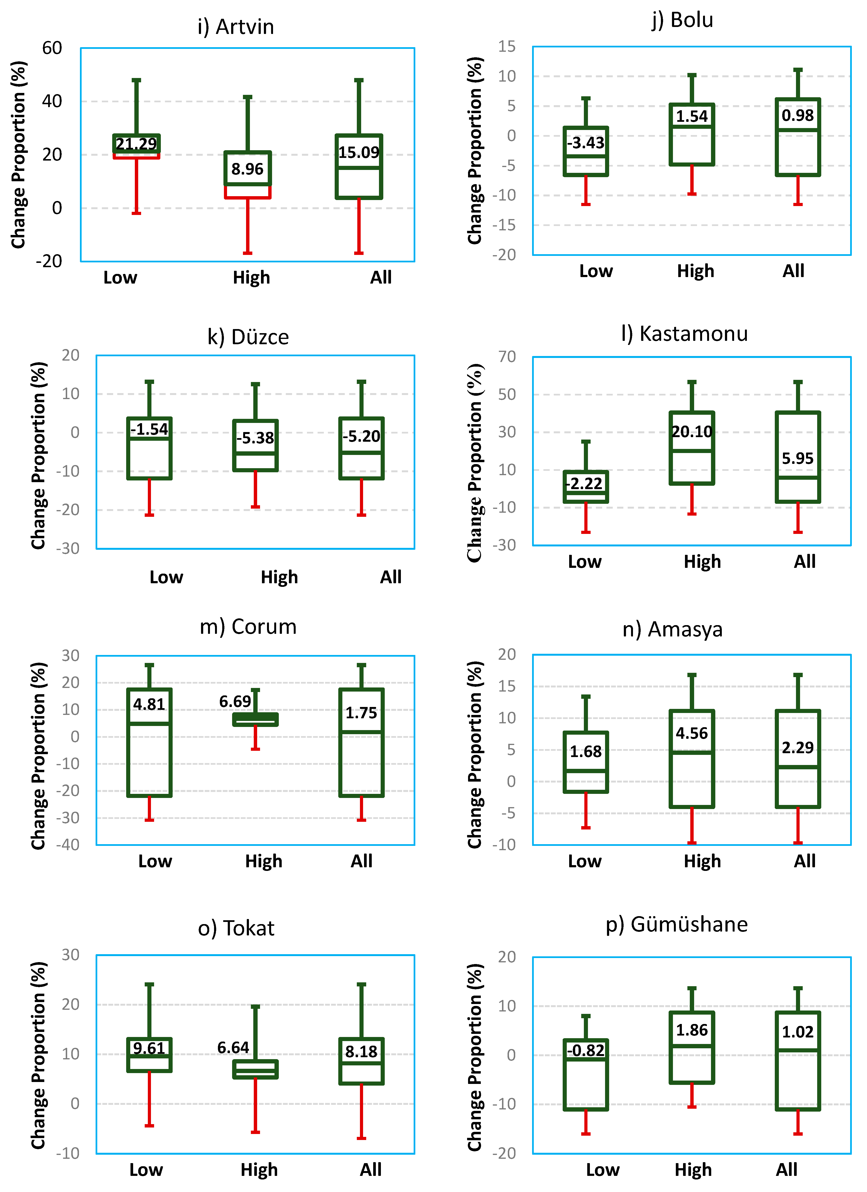
Gumushane	−11.02	−0.82	3.04	−5.58	1.86	8.70	−11.02	1.02	8.70

reports the trend analysis results of annual rainfall using ITA change box (ITA-CB) method proposed by Alashan [30] and corresponding boxes indicating the change proportions for low, medium and all rainfall values are illustrated in Figure 5. As clearly observed from the table and figure, the rainfall data generally have increasing trend similar to MK and CSD test results. High groups of 81% of the stations have increasing trends. This corroborates the projected increase in extreme precipitation in the Middle East for the end of this century [49]. High groups of Samsun, Ordu, and Duzce, low group of Bolu, Duzce, and Gumushane and whole groups of Duzce have decreasing trend only. Low group rainfall of Sinop, Samsun, Ordu, Trabzon, Rize, and Artvin show large increasing trend changes by 46.7%, 17.7%, 18%, 16.69%, 13.4% and 21.29% while the high groups of Zonguldak, Giresun, Trabzon and Kastamonu have change proportions of 15.27%, 13.01%, 12.27%, and 20.1%, respectively. The main advantage of this method is trend change proportions and change rates of low and high values can be visually seen for each rainfall quantile. For example, low group of Corum (Figure 5m) has a small trend change of 4.81% averaged over all quantiles, while the changes for all quantiles of the low group range from −21.8% to 17.53%, all groups of Corum and Gumushane (Figure 5p) have small trend changes of 1.75% and 1.02%, while the changes for all quantiles of the all group range from −21.80% to 17.53% and from −11.02% to 8.70%, respectively.

It is clear from all implemented methods that the annual and seasonal trends variations differ with respect to two different parts of rainfall time series. For example, in CSD analysis, whole annual rainfall series of Sinop has significant upward trend (2.11) while its first and second halves sub-series have negative and low positive trends (−1.52 and 0.36), respectively. In MK analysis also, first and second halves sub-series of Sinop respectively have negative and low positive trends (−1.88 and 0.38) while whole annual rainfall series has significant increasing (2.18). This indicates that trend results considering the full time series can be different from the case when data points within each half of the data period is used for analyses. By this way, stability of trends can also be detected or observed as also found in the present study. As also suggested by Güçlü [30], using partial MK or other methods, more information on trend variability and stability can be drawn from the selected data. The other important issue which is worthy to be noticed here that the industrialization of Turkey especially after 1980s has high effect on climate. In some cities (e.g., Samsun and Zonguldak), high variation in climate and thus, in intensity and duration of rainfall is observed after about 1985. This caused unwanted natural hazards such as floods and droughts [50]. Such effects (e.g., anthropogenic) should also be considered in trend analysis studies.

Results from analyses of changes (e.g., trends and variability) require a careful statistical inference if they are to be considered to support the planning of watershed management practices. If the watershed management plan is in line with the predictive adaptation to the impacts of climate-related changes on hydro-climatology, comprehensive information on the trends in precipitation among other variables such as temperature, and potential evapotranspiration is of paramount importance [51]. The provision of such an information needs to take into account the various sources of uncertainty and how they would affect the results of analyses. When analyzing changes in variables such as rainfall (as considered in this study), findings can be influenced by the choice of a particular method for analyses, errors on observations, etc. [23]. When there are no irregularities in the data (e.g., no ties, no autocorrelation, etc.) the non-parametric methods tend to yield comparable results. For instance, the comparability of MK and Spearman Rho test, and CSD and MK test was demonstrated by Yue et al. [52] and Onyutha [15], respectively. However, differences among methods stem from how they deal with the influence of data irregularities on analyses results [23]. For instance, the assumption of non-parametric methods that the occurrence of data points over time is in an independent and identically distributed way is normally falsified by existence of ties and persistence in the data. Whereas the MK-test tackles the influence of ties through correction of the test statistic variance, instead. the refined graphical-statistical CSD trend test is not affected by ties. Furthermore, how the MK and refined CSD tests deal with the influence of persistence on trend results also differ. This explains the slight difference between the results of the two methods. More interestingly, the assumptions for trend analyses by the non-parametric methods are actually not necessary when applying the ITA approach. So, by detecting trends using various techniques, the influence from the choice of a particular method tends to even out. Besides, the difference in results from the methods highlight the possible uncertainty to be taken into account on the findings.

Relying purely on statistical approach for trend analyses may lead to meaningless results [22]. A graphical approach can reveal fascinating information or hidden features which can invite further investigations to maximize understanding about the data [15]. For instance, the CSD-plot can reveal step jumps in the mean of data, something which the ITA or MK test cannot reveal. The main advantage of the MK and statistical CSD tests being non-parametric in nature is that they do not require the data to be normally distributed. The disadvantage of the MK and CSD tests is that they are conducted under some assumptions which if violated can affect the accuracy of the results. The main disadvantage of the ITA approach is that the data is required to be of even sample size or divisible by two, otherwise a data point is required to be left out. Nevertheless, when several methods are applied to analyze a particular type of change, results from various angles can be obtained. For instance, the ITA approach within a particular analysis shows whether the variable is increasing or decreasing with respect to high, medium, or low values, something which both the MK and refined CSD test do not reveal. On the other hand, when applying the ITA method, it is implied that the sub-trend length is half the data period. However, there are a number of cases that could be revealed by the refined CSD method. For instance, the entire data may be dominated by positive or negative trend and hence no sub-trend. There can be two sub-trends in which the first and the second is less and greater (or vice versa) than half the data period. Instead, there can exist several sub-trends over sub-periods each of which is less than half the data period. In summary, several methods, when applied to analyze changes such as trends in data, yield results which complement each other to lead to a more meaningful inference than in the case with only one method, e.g., the statistical approach used [23]. Some of the studies in which both statistical and graphical trend analyses especially using the MK and CSD tests were applied, including Pirnia et al. [53], Tang et al. [54], Onyutha [55], and Vido et al. [56].

Furthermore, in this study, the data at the various weather stations were more or less over the same period starting from 1960 to 2015. Although it might not always be possible in other studies, data over the same period but from various locations in a region when used for analyses can yield spatially coherent results [57].

4. Conclusions

This study used both the graphical methods of refined CSD and ITA-change boxes and the statistical method of MK for analyzing trends in annual and seasonal precipitation series at 16 stations during 1960–2015 in Turkey. The results reveal a high consistency between the results of the graphical and statistical methods. Comparing the trend results for different seasons, a seasonality was found in precipitation trends, which can be attributed to the contrasting temporal changes in different driving forces of seasonal precipitation. The results also show the trend direction and magnitude of the full time series may be different from the case when the trend is detected in a shorter period (within each half of the data period). It necessitates the use of long-enough time series for historical climate change analyses, as short time series may place on the oscillation high or low periods of the natural climate cycles. The latter may provide misleading information on the hydrological impact of climate change.

A comparison between the graphical and statistical methods indicates that the graphical CSD and ITA methods are capable of identifying the hidden trends in the precipitation time series that cannot be detected using the statistical MK method. It suggests the graphically-oriented trend diagnosis of hydrological changes as a vital complement to rigorous but imperfect traditional statistical methods. In that way, a more detained and comprehensive picture of regional hydrological changes based on quantitative and qualitative analyses is depicted. It will help hydrologists detect the physical mechanisms behind the changes and incorporate them into the decision making and the future planning in the face of anthropogenic-induced changes. Mere reliance on statistical methods which present only yes-or-no answers, i.e., existence or lack of a temporal trend in the time series without any qualitative assessment, increases the risk of decision failure.

References

- Akinsanola, A.A.; Ogunjobi, K.O. Recent homogeneity analysis and long-term spatio-temporal rainfall trends in Nigeria. Theor. Appl. Clim. 2015, 128, 275–289. [Google Scholar] [CrossRef]
- Pendergrass, A.G.; Knutti, R.; Lehner, F.; Deser, C.; Sanderson, B. Precipitation variability increases in a warmer climate. Sci. Rep. 2017, 7, 17966. [Google Scholar] [CrossRef] [PubMed] [Green Version]
- Mathbout, S.; Lopez-Bustins, J.A.; Martin-Vide, J.; Bech, J.; Rodrigo, F.S. Spatial and temporal analysis of drought variability at several time scales in Syria during 1961–2012. Atmos. Res. 2018, 200, 153–168. [Google Scholar] [CrossRef]
- Tabari, H.; Willems, P. More prolonged droughts by the end of the century in the Middle East. Environ. Res. Lett. 2018, 13, 104005. [Google Scholar] [CrossRef] [Green Version]
- Vicente-Serrano, S.M. Differences in Spatial Patterns of Drought on Different Time Scales: An Analysis of the Iberian Peninsula. Water Resour. Manag. 2006, 20, 37–60. [Google Scholar] [CrossRef]
- Doblas-Miranda, E.; Martínez-Vilalta, J.; Lloret, F.; Álvarez, A.; Ávila, A.; Bonet, F.J.; Brotons, L.; Castro, J.; Yuste, J.C.; Díaz, M.; et al. Reassessing global change research priorities in Mediterranean terrestrialecosystems: How far have we come and where do we go from here? Glob. Ecol. Biogeogr. 2015, 24, 25–43. [Google Scholar] [CrossRef] [Green Version]
- Tabari, H.; Willems, P. Lagged influence of Atlantic and Pacific climate patterns on European extreme precipitation. Sci. Rep. 2018, 8, 5748. [Google Scholar] [CrossRef]
- Giorgi, F. Climate change hot-spots. Geophys. Res. Lett. 2006, 33, L08707. [Google Scholar] [CrossRef]
- Tabari, H.; Hosseinzadehtalaei, P.; AghaKouchak, A.; Willems, P. Latitudinal heterogeneity and hotspots of uncertainty in projected extreme precipitation. Environ. Res. Lett. 2019, 14, 124032. [Google Scholar] [CrossRef] [Green Version]
- Ávila, Á.; Guerrero, F.C.; Escobar, Y.C.; Justino, F. Recent Precipitation Trends and Floods in the Colombian Andes. Water 2019, 11, 379. [Google Scholar] [CrossRef] [Green Version]
- McKitrick, R.; Christy, J. Assessing changes in US regional precipitation on multiple time scales. J. Hydrol. 2019, 578, 124074. [Google Scholar] [CrossRef]
- Nashwan, M.; Shahid, S.; Xiaojun, W. Uncertainty in Estimated Trends Using Gridded Rainfall Data: A Case Study of Bangladesh. Water 2019, 11, 349. [Google Scholar] [CrossRef] [Green Version]
- Pandey, B.K.; Khare, D. Identification of trend in long term precipitation and reference evapotranspiration over Narmada river basin (India). Glob. Planet. Chang. 2018, 161, 172–182. [Google Scholar] [CrossRef]
- Tabari, H. Statistical Analysis and Stochastic Modelling of Hydrological Extremes. Water 2019, 11, 1861. [Google Scholar] [CrossRef] [Green Version]
- Onyutha, C. Identification of sub-trends from hydro-meteorological series. Stoch. Environ. Res. Risk Assess. 2015, 30, 189–205. [Google Scholar] [CrossRef]
- Onyutha, C. Statistical analyses of potential evapotranspiration changes over the period 1930–2012 in the Nile River riparian countries. Agric. Forest. Meteorol. 2016, 226–227, 80–95. [Google Scholar] [CrossRef]
- Tabari, H.; Hosseinzadehtalaei, P. Temporal variability of precipitation over Iran: 1966–2005. J. Hydrol. 2011, 396, 313–320. [Google Scholar] [CrossRef]
- Westra, S.; Alexander, L.; Zwiers, F.W. Global Increasing Trends in Annual Maximum Daily Precipitation. J. Clim. 2013, 26, 3904–3918. [Google Scholar] [CrossRef] [Green Version]
- Karandish, F.; Mousavi, S.S.; Tabari, H. Climate change impact on precipitation and cardinal temperatures in different climatic zones in Iran: Analyzing the probable effects on cereal water-use efficiency. Stoch. Environ. Res. Risk Assess. 2016, 31, 2121–2146. [Google Scholar] [CrossRef]
- Shiru, M.S.; Shahid, S.; Chung, E.S.; Alias, N. Changing characteristics of meteorological droughts in Nigeria during 1901–2010. Atmos. Res. 2019, 223, 60–67. [Google Scholar] [CrossRef]
- Dudley, R.; Hirsch, R.; Archfield, S.; Blum, A.; Renard, B. Low streamflow trends at human-impacted and reference basins in the United States. J. Hydrol. 2020, 580, 124254. [Google Scholar] [CrossRef]
- Kundzewicz, Z.W.; Robson, A. Detecting Trend and Other Changes in Hydrological Data; World Climate Program—Water, WMO/UNESCO, WCDMP-45, WMO/TD-No.1013; WMO: Geneva, The Netherlands, 2000; p. 157. [Google Scholar]
- Onyutha, C. Statistical Uncertainty in Hydrometeorological Trend Analyses. Adv. Meteorol. 2016, 2016, 1–26. [Google Scholar] [CrossRef] [Green Version]
- Wu, H.; Qian, H. Innovative trend analysis of annual and seasonal rainfall and extreme values in Shaanxi, China, since the 1950s. Int. J. Clim. 2016, 37, 2582–2592. [Google Scholar] [CrossRef]
- Wang, X.; Xiao, J.; Li, X.; Cheng, G.; Ma, M.; Zhu, G.; Arain, M.A.; Black, T.A.; Jassal, R.S. No trends in spring and autumn phenology during the global warming hiatus. Nat. Commun. 2019, 10, 2389. [Google Scholar] [CrossRef] [PubMed]
- Sen, Z. An innovative trend analysis methodology. J. Hydrol. Eng. 2012, 17, 1042–1046. [Google Scholar] [CrossRef]
- Onyutha, C. An improved method to quantify trend slope and its significance. Front. Earth Sci. 2020; under review. [Google Scholar]
- Şen, Z. Trend identification simulation and application. J. Hydrol. Eng. 2014, 19, 635–642. [Google Scholar] [CrossRef]
- Şen, Z. Innovative trend significance test and applications. Theor. Appl. Clim. 2015, 127, 939–947. [Google Scholar] [CrossRef]
- Güçlü, Y.S. Multiple Şen-innovative trend analyses and partial Mann-Kendall test. J. Hydrol. 2018, 566, 685–704. [Google Scholar] [CrossRef]
- Alashan, S. An improved version of innovative trend analyses. Arab. J. Geosci. 2018, 11, 50. [Google Scholar] [CrossRef]
- Güçlü, Y.S.; Dabanli, I.; Sisman, E.; Sen, Z. Air quality (AQ) identification by innovative trend diagram and AQ index combinations in Istanbul megacity. Atmospheric Pollut. Res. 2019, 10, 88–96. [Google Scholar] [CrossRef]
- Tabari, H.; Taye, M.T.; Onyutha, C.; Willems, P. Decadal Analysis of River Flow Extremes Using Quantile-Based Approaches. Water Resour. Manag. 2017, 2, 527–3387. [Google Scholar] [CrossRef]
- Öztopal, A.; Şen, Z. Innovative Trend Methodology Applications to Precipitation Records in Turkey. Water Resour. Manag. 2016, 31, 727–737. [Google Scholar] [CrossRef]
- Şen, Z. Innovative Trend Methodologies in Science and Engineering. In Innovative Trend Methodologies in Science and Engineering; Springer: Cham, Switzerland, 2017. [Google Scholar]
- Mohorji, A.M.; Şen, Z.; Almazroui, M. Trend Analyses Revision and Global Monthly Temperature Innovative Multi-Duration Analysis. Earth Syst. Environ. 2017, 1, 9. [Google Scholar] [CrossRef] [Green Version]
- Amrhein, V.; Greenland, S.; McShane, B. Scientists rise up against statistical significance. Nature 2019, 567, 305–307. [Google Scholar] [CrossRef] [Green Version]
- Deniz, A.; Toros, H.; Incecik, S. Spatial variations of climate indices in Turkey. Int. J. Clim. 2011, 31, 394–403. [Google Scholar] [CrossRef]
- Duzenli, E.; Tabari, H.; Willems, P.; Yilmaz, M.T. Decadal variability analysis of extreme precipitation in Turkey and its relationship with teleconnection patterns. Hydrol. Process. 2018, 32, 3513–3528. [Google Scholar] [CrossRef]
- Sensoy, S.; Demircan, M.; Ulupınar, U.; Balta, I. Turkey Climate. DMI. 2008. Available online: http://www.dmi.gov.tr/iklim/iklim.aspx (accessed on 20 February 2020). (In Turkish)
- Akçar, N.; Yavuz, V.; Ivy-Ochs, S.; Kubik, P.W.; Vardar, M.; Schlüchter, C. Palaeoglacial records from Kavron Valley, NE Turkey: Field and cosmogenic exposure dating evidence. Quat. Int. 2007, 164, 170–183. [Google Scholar] [CrossRef]
- Tatli, H.; Dalfes, N.; Menteş, S. A statistical downscaling method for monthly total precipitation over Turkey. Int. J. Clim. 2004, 24, 161–180. [Google Scholar] [CrossRef]
- Sariş, F.; Hannah, D.M.; Eastwood, W.J. Spatial variability of precipitation regimes over Turkey. Hydrol. Sci. J. 2010, 55, 234–249. [Google Scholar] [CrossRef] [Green Version]
- Biyik, G.; Unal, Y.; Onol, B. Assessment of Precipitation Forecast Accuracy over Eastern Black Sea Region using WRF-ARW. In Proceedings of the 11th Plinius Conference on Mediterranean Storms, Barcelona, Spain, 7–10 September 2009. [Google Scholar]
- Mann, H.B. Nonparametric Tests against Trend. Econometrica 1945, 13, 245. [Google Scholar] [CrossRef]
- Kendall, M.G. Rank Correlation Methods, 4th ed.; Griffin, C., Ed.; Griffin: London, UK, 1975. [Google Scholar]
- Theil, H. A rank-invariant method of linear and polynomial regression analysis. Nederl. Akad. Wetench. Ser. A 1950, 53, 386–392. [Google Scholar]
- Sen, P.K. Estimates of the regression coefficient based on Kendall’s tau. J. Am. Stat. Assoc. 1968, 63, 1379–1389. [Google Scholar] [CrossRef]
- Tabari, H.; Willems, P. Seasonally varying footprint of climate change on precipitation in the Middle East. Sci. Rep. 2018, 8, 4435. [Google Scholar] [CrossRef] [PubMed]
- Baglee, A.; Connell, R.; Haworth, A.; Rabb, B.; Bugler, W.; Ulug, G.; Capalov, L.; Hansen, D.S.; Glenting, C.; Jensen, C.H.; et al. Climate Risk Case Study, Plot Climate Change Adaptation Market Study: Turkey. 2013. Available online: https://www.ebrd.com/downloads/sector/sei/turkey-adaptation-study.pdf (accessed on 20 February 2020).
- Onyutha, C.; Tabari, H.; Rutkowska, A.; Nyeko-Ogiramoi, P.; Willems, P. Comparison of different statistical downscaling methods for climate change rainfall projections over the Lake Victoria basin considering CMIP3 and CMIP5. HydroResearch 2016, 12, 31–45. [Google Scholar] [CrossRef]
- Yue, S.; Pilon, P.; Cavadias, G. Power of the Mann–Kendall and Spearman’s rho tests for detecting monotonic trends in hydrological series. J. Hydrol. 2002, 259, 254–271. [Google Scholar] [CrossRef]
- Pirnia, A.; Golshan, M.; Darabi, H.; Adamowski, J.F.; Rozbeh, S. Using the Mann–Kendall test and double mass curve method to explore stream flow changes in response to climate and human activities. J. Water Clim. Chang. 2018, 10, 725–742. [Google Scholar] [CrossRef]
- Tang, L.; Zhang, Y. Considering Abrupt Change in Rainfall for Flood Season Division: A Case Study of the Zhangjia Zhuang Reservoir, Based on a New Model. Water 2018, 10, 1152. [Google Scholar] [CrossRef] [Green Version]
- Onyutha, C. Trends and variability in African long-term precipitation. Stoch. Environ. Res. Risk Assess. 2018, 32, 2721–2739. [Google Scholar] [CrossRef]
- Vido, J.; Nalevanková, P.; Valach, J.; Šustek, Z.; Tadesse, T. Drought Analyses of the Horné Požitavie Region (Slovakia) in the Period 1966–2013. Adv. Meteorol. 2019, 2019, 1–10. [Google Scholar] [CrossRef]
- Onyutha, C.; Tabari, H.; Taye, M.T.; Nyandwaro, G.N.; Willems, P. Analyses of rainfall trends in the Nile River Basin. HydroResearch 2016, 13, 36–51. [Google Scholar] [CrossRef]
Figure 1.
Locations of precipitation gauging stations used in the study.
Figure 2.
Histograms of the monthly precipitations for the stations under study.
Figure 3.
CSD-plot for annual rainfall at stations (a–p) selected across the study area.
Figure 4.
CSD-based graphical diagnoses of the trend significance for annual rainfall at stations (a–p) selected across the study area.
Figure 5.
Annual trend graphs at the study stations using the ITA-CB.