Identifying Spatially Correlated Patterns between Surface Water and Frost Risk Using EO Data and Geospatial Indices

 , ,
, ,  and
and
Abstract
:1. Introduction
2. Materials and Methods
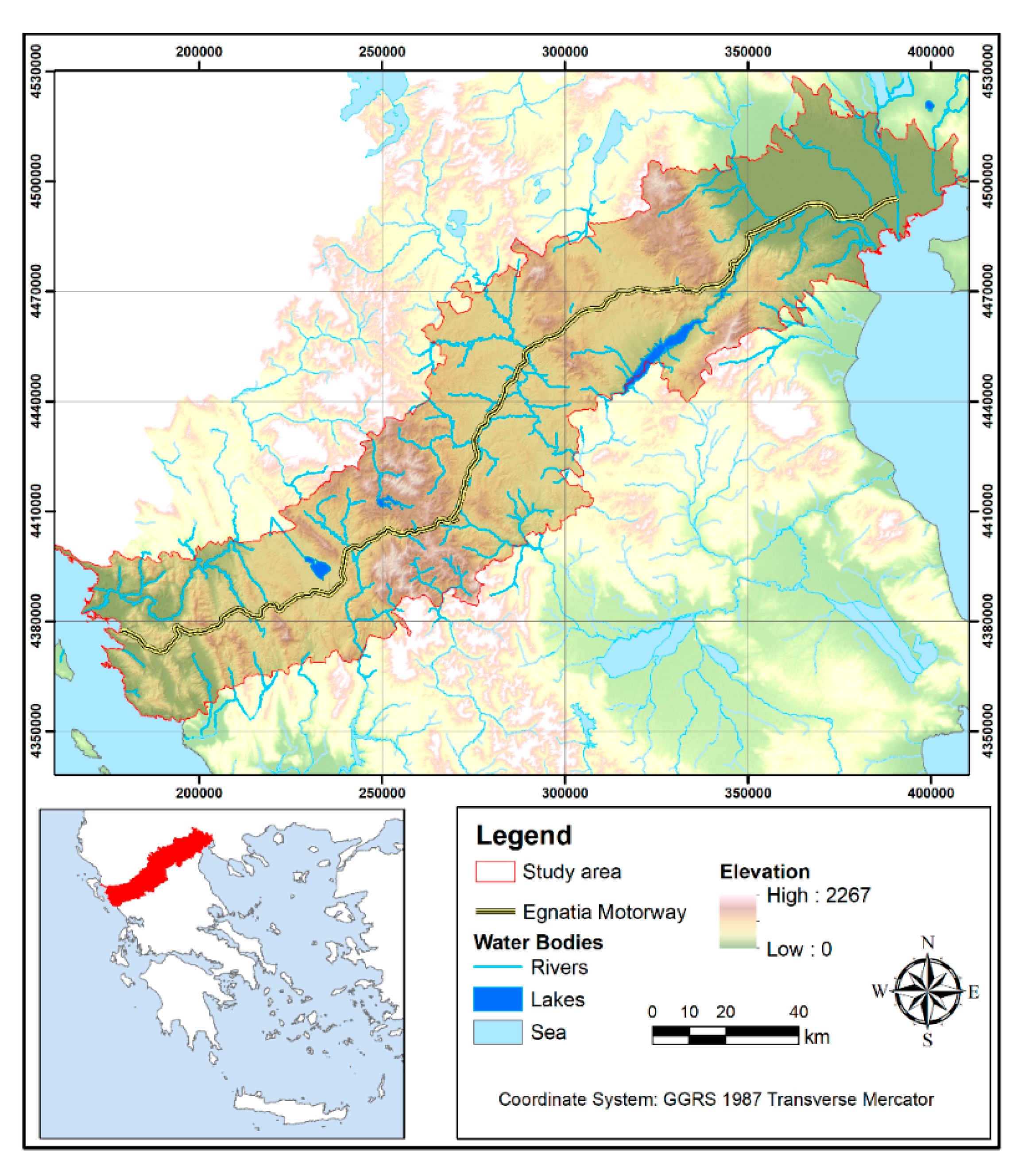
2.1. Study Area
2.2. Data
2.3. Methodology
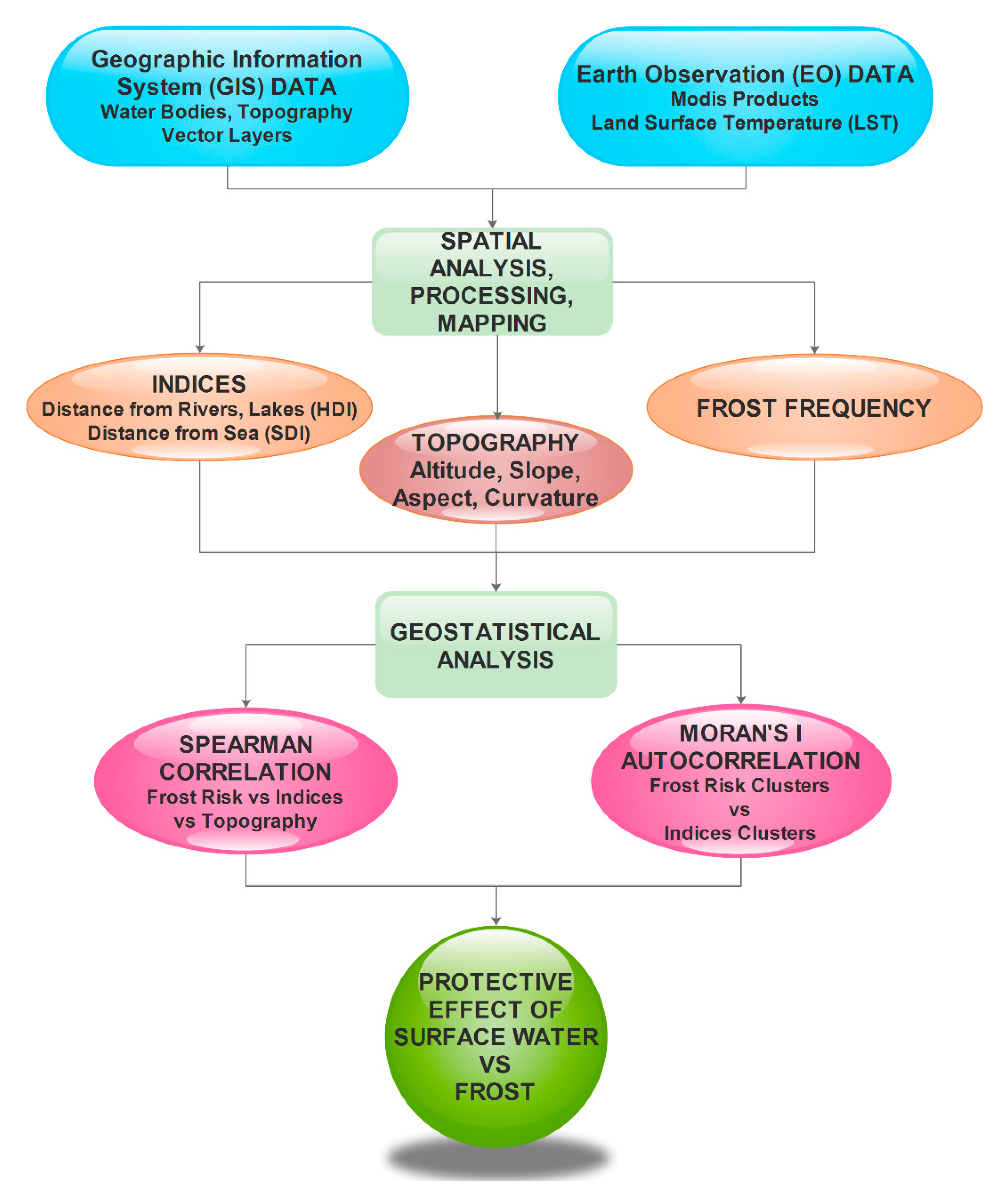
2.3.1. Overview
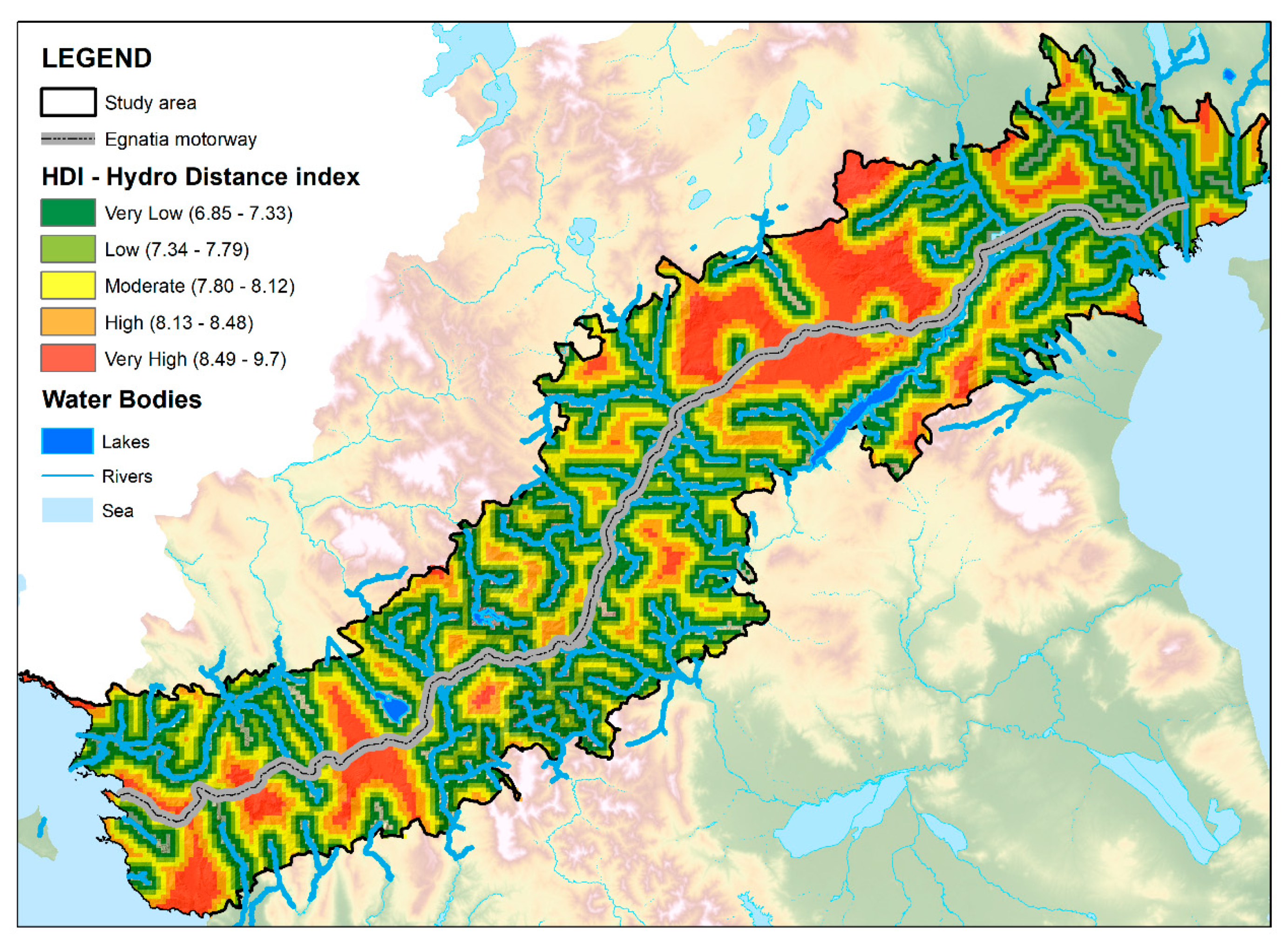
2.3.2. Spatial Analysis of Water Bodies and Development of Indices
2.3.3. Frost Frequency Analysis
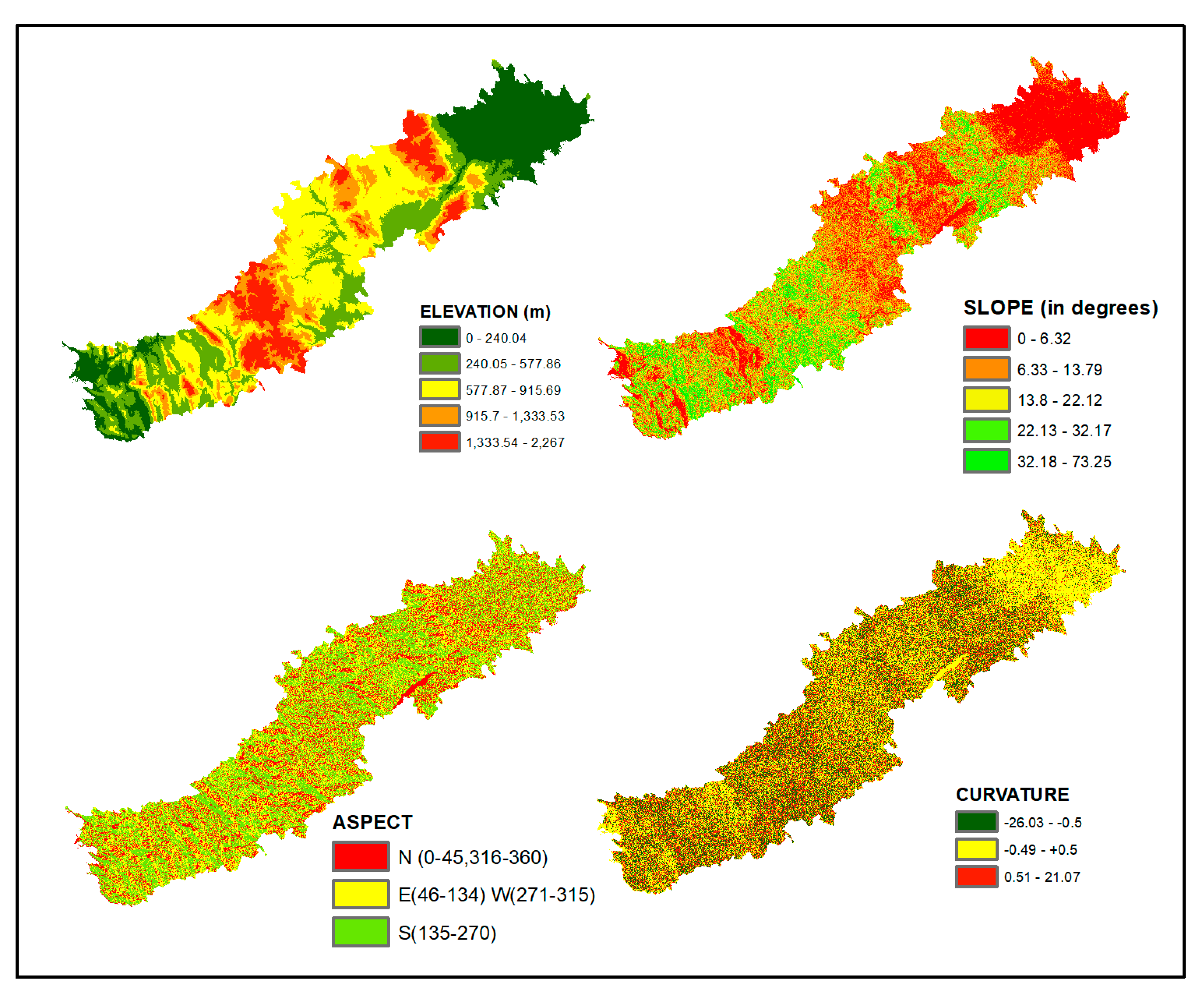
2.3.4. Topography Analysis
2.3.5. Statistical Analysis
2.3.6. Moran’s I Autocorrelation Analysis
3. Results
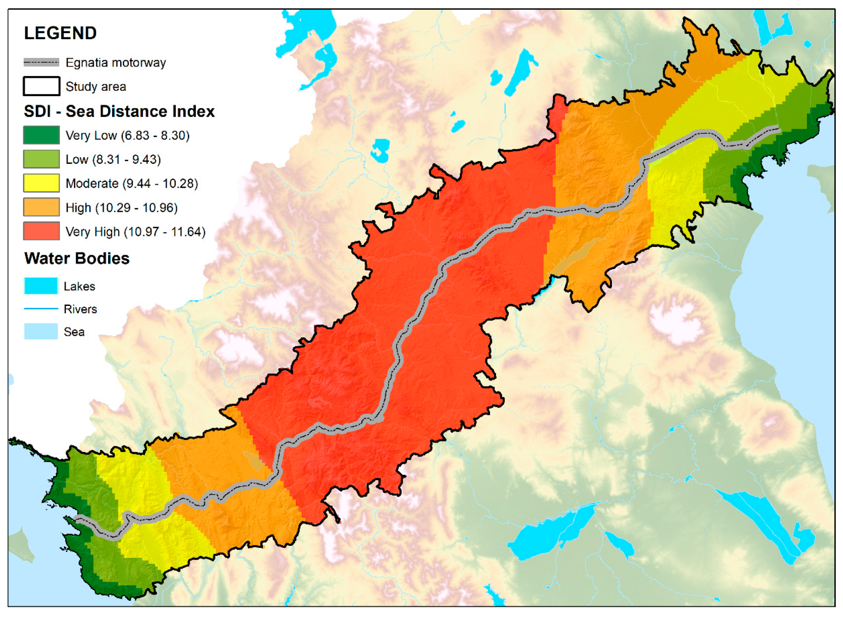
3.1. Spatial Distribution of HDI and SDI
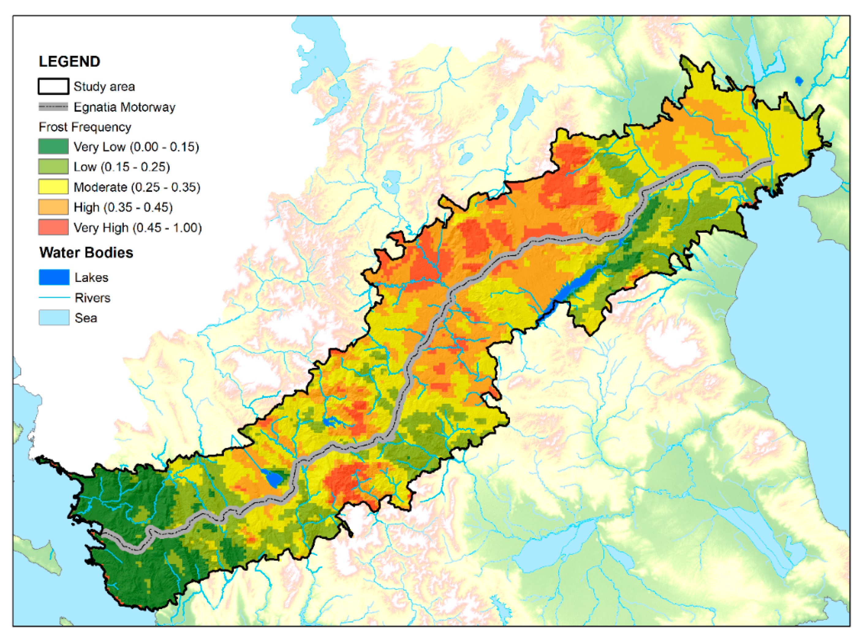
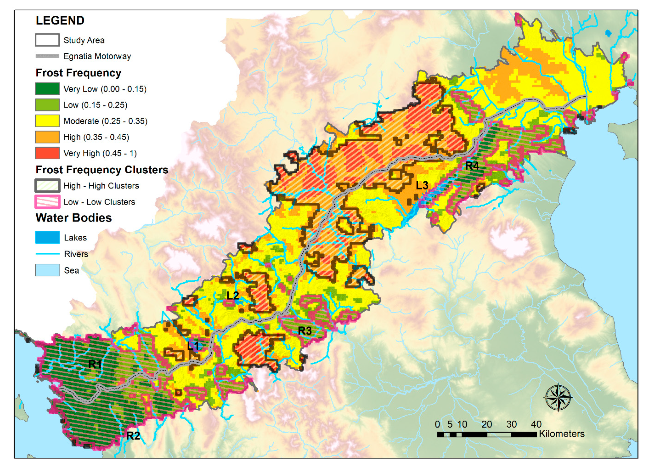
3.2. Spatial Distribution of Frost Frequency
3.3. Statistical Analysis
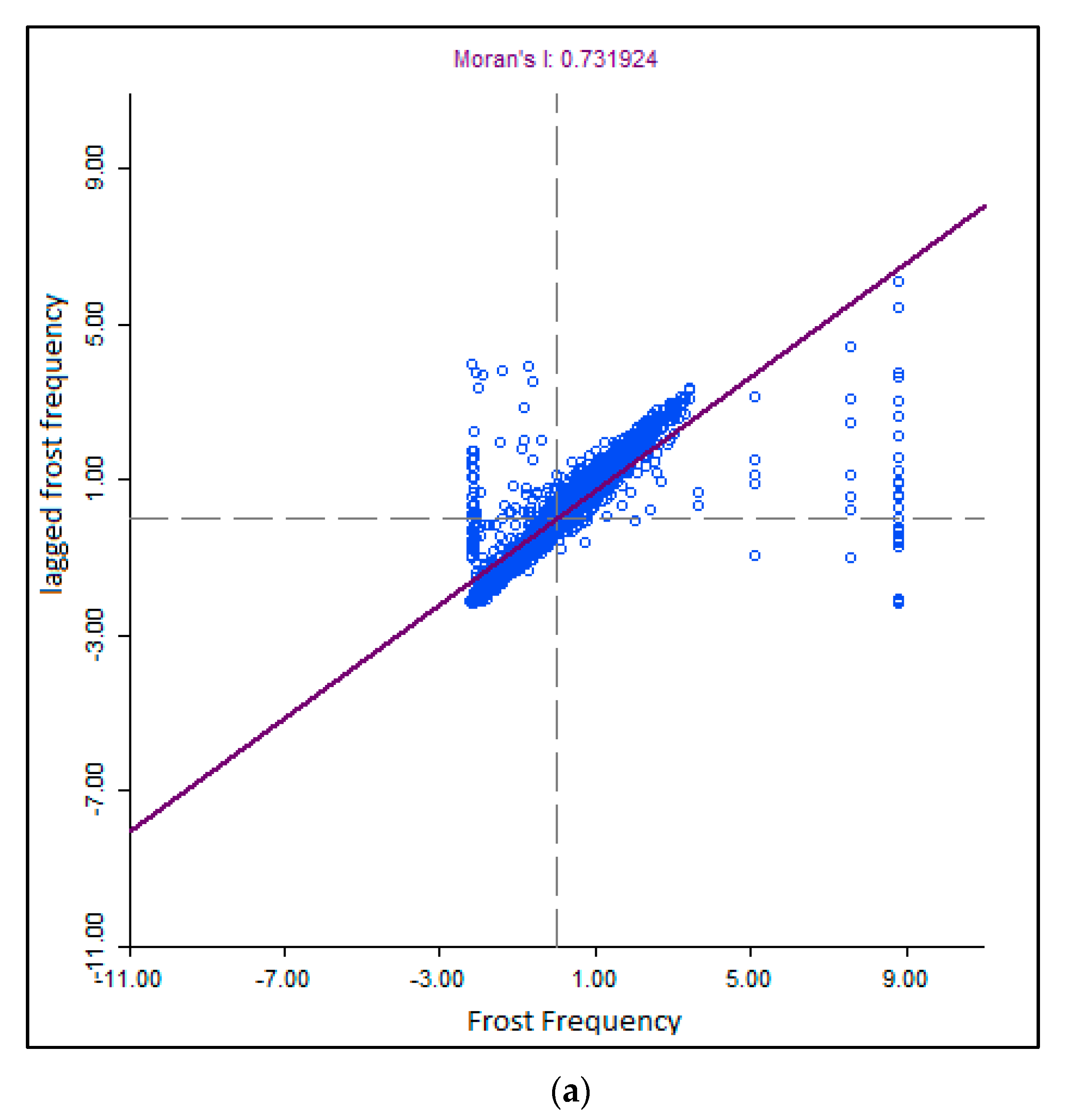
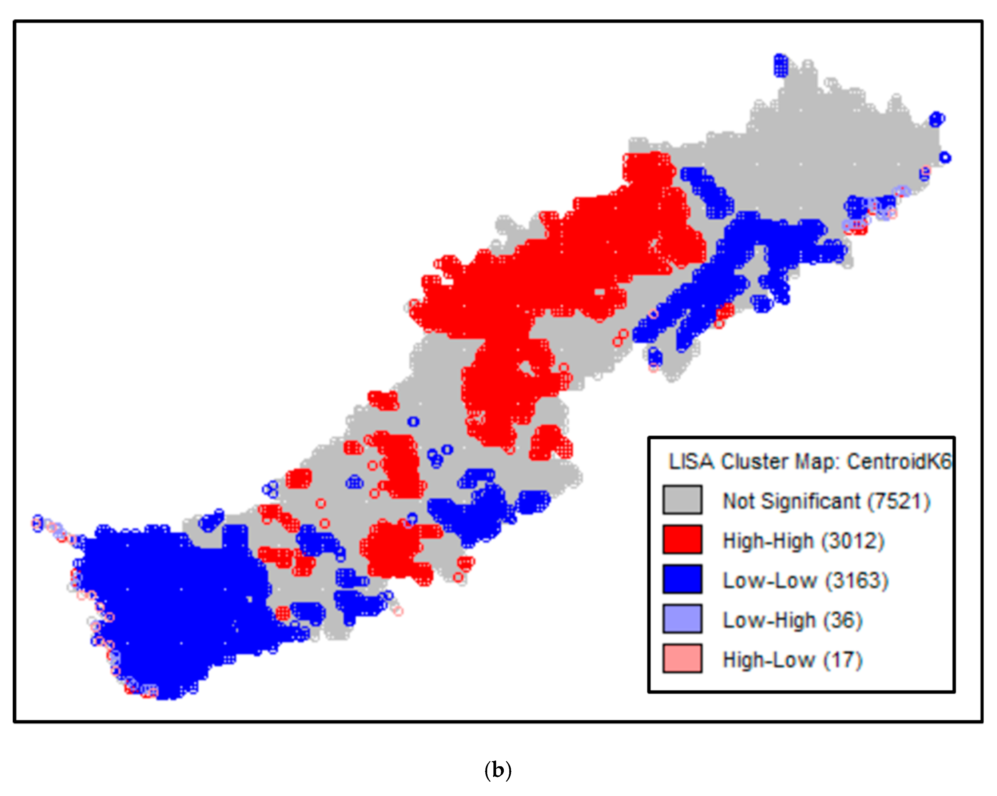
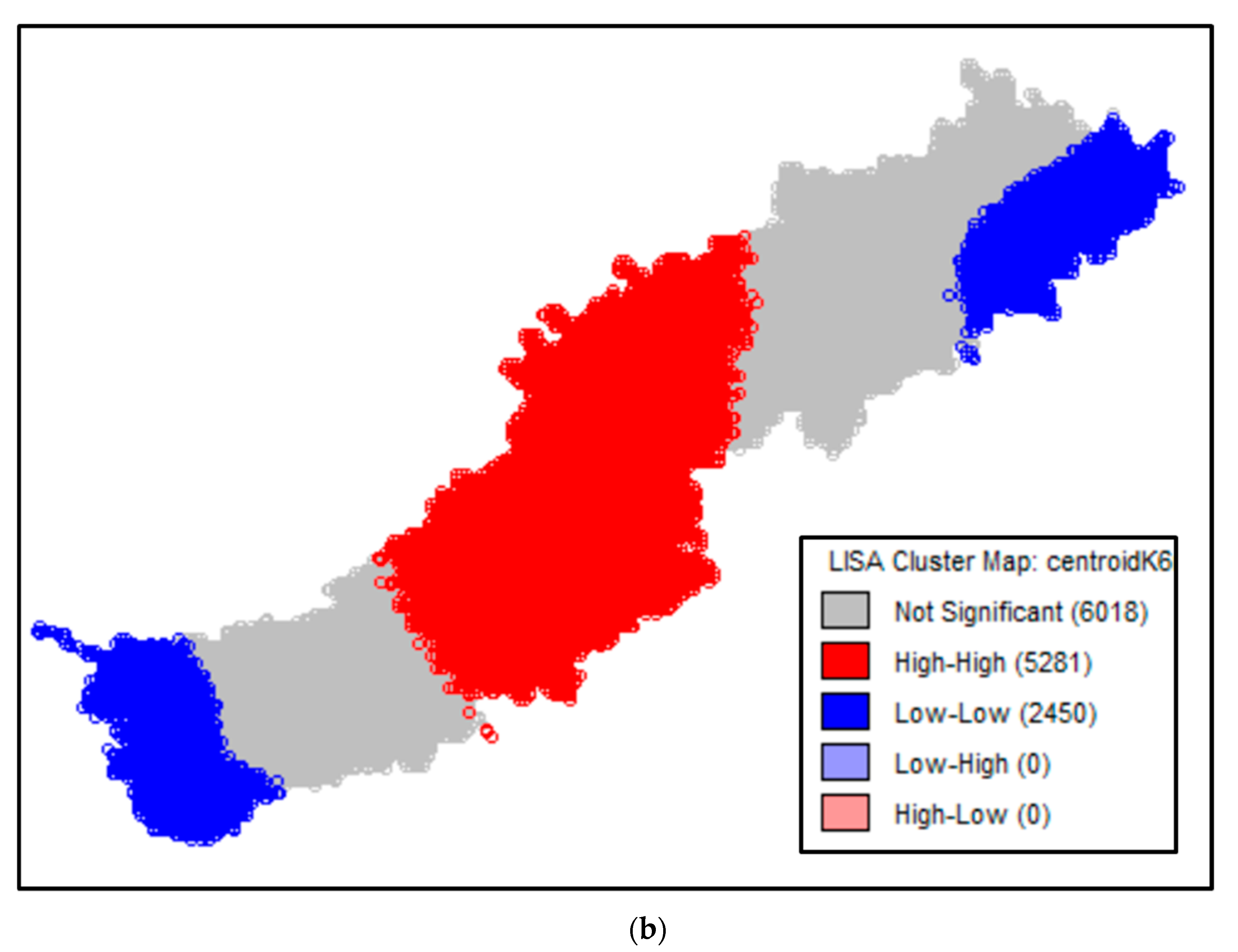
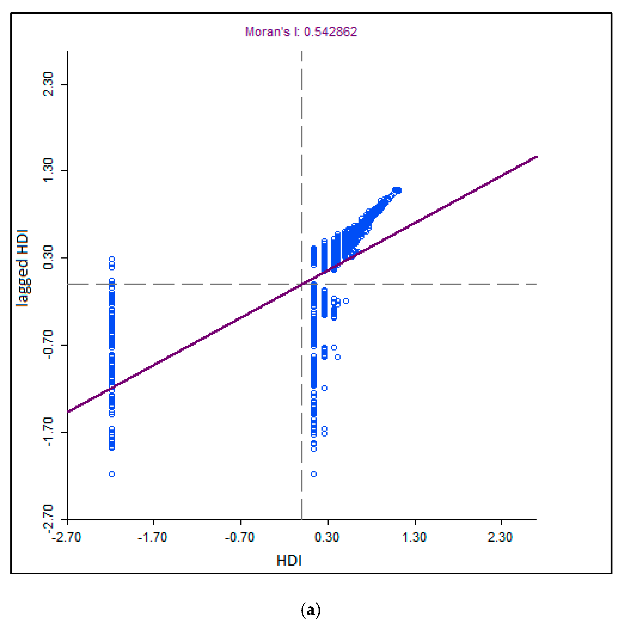
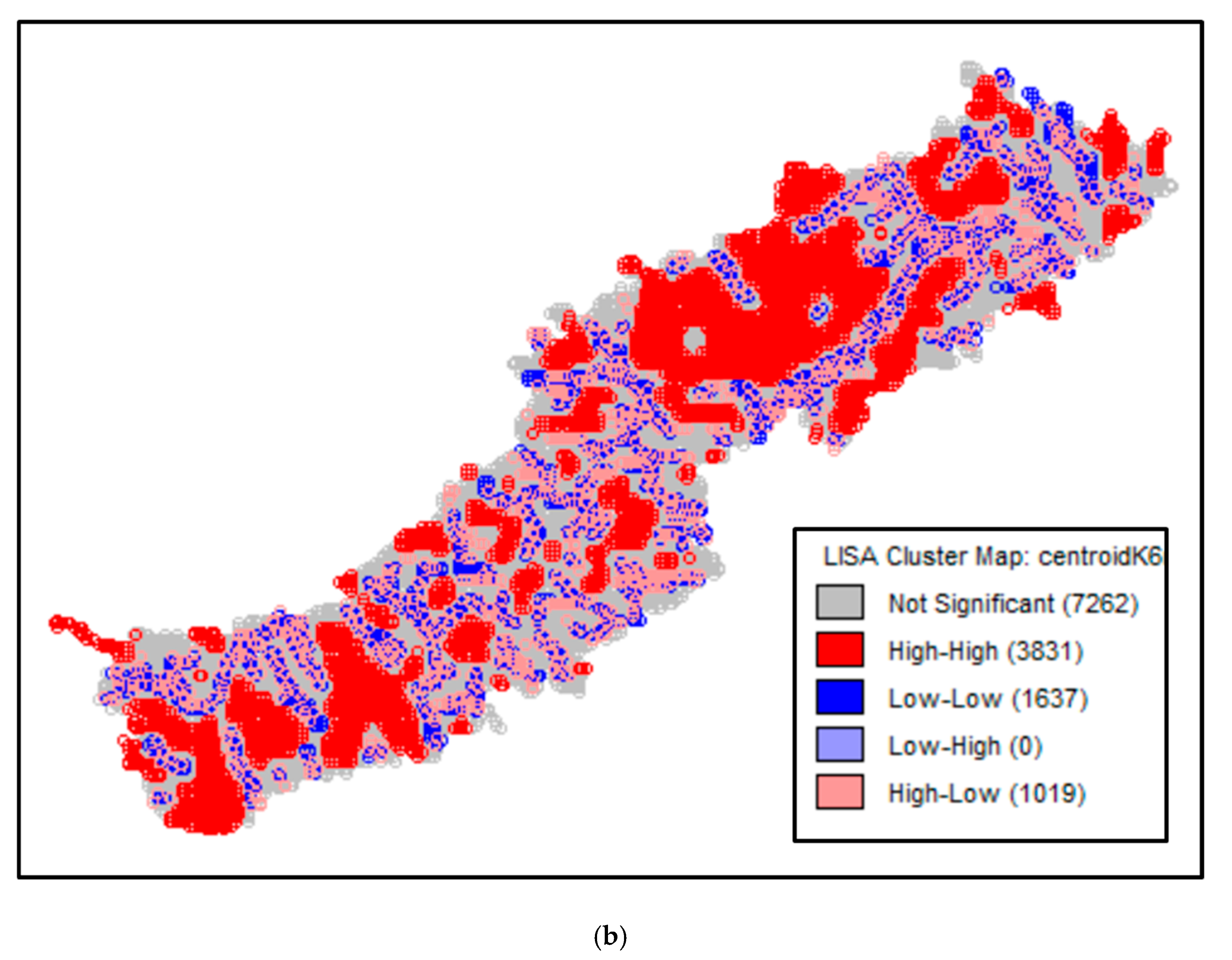
3.4. Spatial Autocorrelation
4. Discussion
5. Conclusions
Author Contributions
Funding
Conflicts of Interest
References
- Kalogeropoulos, K.; Chalkias, C. Modelling the impacts of climate change on surface runoff in small Mediterranean catchments: Empirical evidence from Greece. Water Environ. J. 2013, 27, 505–513. [Google Scholar] [CrossRef]
- Pulvirenti, L.; Pierdicca, N.; Chini, M.; Guerriero, L. An algorithm for operational flood mapping from Synthetic Aperture Radar (SAR) data using fuzzy logic. Nat. Hazards Earth Syst. Sci. 2011, 11, 529–540. [Google Scholar] [CrossRef] [Green Version]
- Skakun, S.; Kussul, N.; Shelestov, A.; Kussul, O. Flood Hazard and Flood Risk Assessment Using a Time Series of Satellite Images: A Case Study in Namibia. Risk Anal. 2014, 34, 1521–1537. [Google Scholar] [CrossRef] [PubMed]
- Stathopoulos, N.; Kalogeropoulos, K.; Polykretis, C.; Skrimizeas, P.; Louka, P.; Karymbalis, E.; Chalkias, C. Introducing Flood Susceptibility Index Using RS Data & GIS—Empirical Analysis in Sperchios River Basin, Greece. In Remote Sensing of Hydro-Meteorological Hazards, 1st ed.; Petropoulos, G.P., Islam, T., Eds.; CRC Press: Boca Raton, FL, USA, 2017; Volume 1, pp. 381–400. [Google Scholar] [CrossRef]
- Stathopoulos, N.; Lykoudi, E.; Vasileiou, E.; Rozos, D.; Dimitrakopoulos, D. Erosion Vulnerability Assessment of Sperchios River Basin, in East Central Greece—A GIS Based Analysis. Open J. Geol. 2017, 7, 621–646. [Google Scholar] [CrossRef] [Green Version]
- Stathopoulos, N.; Kalogeropoulos, K.; Dimitriou, E.; Skrimizeas, P.; Louka, P.; Papadias, V.; Chalkias, C. A Robust Remote Sensing–Spatial Modeling–Remote Sensing (RMR) Approach for Flood Hazard Assessment. In Spatial Modeling in GIS and R for Earth and Environmental Sciences, 1st ed.; Pourghasemi, H.R., Gokceoglu, C., Eds.; Elsevier: Amsterdam, The Netherlands, 2019; Volume 1, pp. 391–410. [Google Scholar] [CrossRef]
- Fridley, J.D. Downscaling Climate over complex Terrain: High Finescale (<1.000 m) Spatial Variation of Near-Ground Temperatures in a Montane Forested Landscape (Great Smoky Mountains). J. Appl. Meteorol. Clim. 2009, 48, 1033–1049. [Google Scholar] [CrossRef] [Green Version]
- Pouteau, R.; Rambal, S.; Ratte, J.P.; Goge, F.; Joffre, R.; Winkel, T. Downscaling MODIS-derived maps using GIS and boosted regression trees: The case of frost occurrence over the arid Andean highlands of Bolivia. Remote Sens. Environ. 2011, 115, 117–129. [Google Scholar] [CrossRef] [Green Version]
- Daly, C.; Halbleib, M.; Smith, J.I.; Gibson, W.P.; Doggett, M.K.; Taylor, G.H.; Pasteris, P.P. Physiographically sensitive mapping of climatological temperature and precipitation across the conterminous United States. Intern. J. Climatol. J. Roy. Meteor. Soc. 2008, 28, 2031–2064. [Google Scholar] [CrossRef]
- Holdaway, M. Spatial modeling and interpolation of monthly temperature using kriging. Clim. Res. 1996, 6, 215–225. [Google Scholar] [CrossRef] [Green Version]
- Daly, C.; Gibson, W.P.; Taylor, G.H.; Johnson, G.L.; Pasteris, P. A knowledge-based approach to the statistical mapping of climate. Clim. Res. 2002, 22, 99–113. [Google Scholar] [CrossRef] [Green Version]
- Vercauteren, N.; Destouni, G.; Dahlberg, C.J.; Hylander, K. Fine-resolved, near-coastal spatiotemporal variation of temperature in response to insolation. J. Appl. Meteorol. Clim. 2013, 52, 1208–1220. [Google Scholar] [CrossRef]
- Ashcroft, M.B.; Chisholm, L.A.; French, K.O. The effect of exposure on landscape scale soil surface temperatures and species distribution models. Landsc. Ecol. 2008, 23, 211–225. [Google Scholar] [CrossRef] [Green Version]
- Ashcroft, M.B.; Gollan, J.R. Fine—Resolution (25 m) topoclimatic grids of near—Surface (5 cm) extreme temperatures and humidities across various habitats in a large (200 × 300 km) and diverse region. Int. J. Climatol. 2012, 32, 2134–2148. [Google Scholar] [CrossRef] [Green Version]
- Suggitt, A.J.; Gillingham, P.K.; Hill, J.K.; Huntley, B.; Kunin, W.E.; Roy, D.B.; Thomas, C.D. Habitat microclimates drive fine-scale variation in extreme temperatures. Oikos 2011, 120, 1–8. [Google Scholar] [CrossRef]
- Francois, C.; Bosseno, R.; Vacher, J.J.; Segiun, B. Frost risk mapping derived from satellite and surface data over the Bolivian Altiplano. Agric. For. Meteorol. 1999, 95, 113–137. [Google Scholar] [CrossRef]
- Blennow, K.; Persson, P. Modeling local-scale frost variations using mobile temperature measurements with GIS. Agric. For. Meteorol. 1998, 89, 59–71. [Google Scholar] [CrossRef]
- Kerdiles, H.; Grondona, M.; Rodriguez, R.; Seguin, B. Frost mapping using NOAA AVHRR data in the Papean region, Argentina. Agric. For. Meteorol. 1996, 79, 157–182. [Google Scholar] [CrossRef]
- Lindkvist, L.; Gustavsson, T.; Borgen, J. A frost assessment method for mountainous areas. Agric. Forest Meteorol. 2000, 102, 51–67. [Google Scholar] [CrossRef]
- Rigby, J.R.; Porporato, A. Spring frost risk in a changing climate. Geophys. Res. Lett. 2008, 35. [Google Scholar] [CrossRef]
- Cooper, W.C.; Young, R.H.; Turrell, F.M. Microclimate and physiology of citrus: Their relation to cold protection. Agric. Sci. Rev. 1964, 2, 38–50. [Google Scholar]
- Hewitt, K. The idea of calamity in a technocratic age. In Interpretations of Calamity from the Viewpoint of Human Ecology, 1st ed.; Hewitt, K., Ed.; Allen & Unwin Inc.: Boston, MA, USA, 1983; Volume 1, pp. 3–32. [Google Scholar]
- Stebelsky, I. Wheat yields and weather hazards in the Soviet Union. In Interpretations of Calamity from the Viewpoint of Human Ecology, 1st ed.; Hewitt, K., Ed.; Allen & Unwin Inc.: Boston, MA, USA, 1983; Volume 1, pp. 202–218. [Google Scholar] [CrossRef]
- Martsole, J.D.; Gerber, J.F.; Chen, E.Y.; Jackson, J.L.; Rose, A.J. What do satellite and other data suggest about past and future Florida freezes. In Proceedings of the Annual Meeting of the Florida State Horticulture Society, Fresno, CA, USA, 18–21 November 1985; Volume 97, pp. 17–21. [Google Scholar]
- Caprio, J.M.; Snyder, R.D. Study to Improve Winterkill Parameters for a Winter Wheat Model. Task 1, a Study of the Relation between Soil Temperature at Three Centimeter Depth and Air Temperature; Final Project Report. NASA Contract NAS9-16007; Plant and Soil Science Department, Montana State University: Bozeman, MT, USA, 1984; p. 76. [Google Scholar]
- Cox, D.L.; Larsen, J.K.; Brun, L.J. Winter survival response of winter wheat: Tillage and cultivar selection 1. Agron. J. 1986, 78, 795–801. [Google Scholar] [CrossRef]
- Condori, B.; Hijmans, R.J.; Ledent, J.F.; Quiroz, R. Managing Potato Biodiversity to Cope with Frost Risk in the High Andes: A Modeling Perspective. PLoS ONE 2014, 9, e81510. [Google Scholar] [CrossRef] [PubMed] [Green Version]
- Snyder, R.L.; Melo-Abreu, J.D. Frost Protection: Fundamentals, Practice and Economics; Food and Agriculture Organization of the United Nations: Rome, Italy, 2005; Volume 1, pp. 1–240. [Google Scholar]
- Larcher, W. Ökophysiologie der Pflanzen 2001 Stuttgart; Eugen Ulmer: Stuttgart, Germany, 2001; p. 302. [Google Scholar]
- Eriksson, M. Winter road climate investigations using GIS. Doctoral Thesis, University of Gothenburg, Gothenburg, Sweden, 2001. [Google Scholar]
- Shao, J.; Lister, P.J. The prediction of Road Surface State and Simulation of the Shading Effect. Bound. Lay. Meteorol. 1995, 73, 411–419. [Google Scholar] [CrossRef]
- Louka, P.; Papanikolaou, I.; Petropoulos, G.P.; Stathopoulos, N. Temperature Fluctuation & Frost Risk Analysis on a Road Network, by Coupling Remote Sensing Data, Thermal Mapping and GIS Techniques. In Remote Sensing of Hydro-Meteorological Hazards, 1st ed.; Petropoulos, G.P., Islam, T., Eds.; CRC Press: Boca Raton, FL, USA, 2017; Volume 1, pp. 183–210. [Google Scholar] [CrossRef]
- Chuanyan, Z.; Zhongren, N.; Guodong, C. Methods for modelling of temporal and spatial distribution of air temperature at landscape scale in the southern Qilian mountains, China. Ecol. Model. 2005, 189, 209–220. [Google Scholar] [CrossRef]
- Tomlinson, C.J.; Chapman, L.; Thornes, J.E.; Baker, C. Remote sensing land surface temperature for meteorology and climatology: A review. Meteorol. Appl. 2011, 18, 296–306. [Google Scholar] [CrossRef] [Green Version]
- Dubayah, R. Modeling a solar radiation topoclimatology for the Rio Grande River Basin. J. Veg. Sci. 1994, 5, 627–640. [Google Scholar] [CrossRef]
- Dubayah, R.; Rich, P.M. Topographic solar radiation models for GIS. Int. J. Geogr. Inf. Syst. 1995, 9, 405–419. [Google Scholar] [CrossRef]
- Safanda, J. Ground surface temperature as a function of slope angle and slope orientation and its effect on the subsurface temperature field. Tectonophysics 1999, 306, 367–375. [Google Scholar] [CrossRef]
- Chapman, L.; Thornes, J.E.; Bradley, A.V. Modelling of road surface temperature from a geographical database. Part 2: Numerical. Meteorol. Appl. 2001, 8, 421–436. [Google Scholar] [CrossRef]
- Jarvis, C.H.; Stuart, N. A comparison among strategies for interpolating maximum and minimum daily air temperatures. Part I: The selection of “guiding” topographic and land cover variables. J. Appl. Meteorol. 2001, 40, 1060–1074. [Google Scholar] [CrossRef]
- Lookingbill, T.R.; Urban, D.L. Spatial estimation of air temperature differences for landscape-scale studies in montane environments. Agric. For. Meteorol. 2003, 114, 141–151. [Google Scholar] [CrossRef]
- Chapman, L.; Thornes, J.E. Road Ice prediction using geomatics. Sci. Total Environ. 360 2006, 1–3, 68–80. [Google Scholar] [CrossRef]
- Bennie, J.; Kubin, E.; Wiltshire, A.; Huntley, B.; Baxter, R. Predicting spatial and temporal patterns of bud-burst and spring frost risk in north-west Europe: The implications of local adaptation to climate. Glob. Chang. Biol. 2010, 16, 1503–1514. [Google Scholar] [CrossRef]
- Erlat, E.; Türkeş, M. Analysis of observed variability and trends in numbers of frost days in Turkey for the period 1950-2010. Int. J. Climatol. 2011, 32, 1889–1898. [Google Scholar] [CrossRef]
- Stroppiana, D.; Antoninetti, M.; Brivio, P.A. Seasonality of MODIS LST over Southern Italy and correlation with land cover, topography and solar radiation. Eur. J. Remote Sens. 2014, 47, 133–152. [Google Scholar] [CrossRef]
- Van de Kerchove, R.; Lhermitte, S.; Veraverbeke, S.; Goossens, R. Spatio-temporal variability in remotely sensed land surface temperature and its relationship with physiographic variables in the Russian Altay Mountains. Int. J. Appl. Earth Obs. 2013, 20, 4–19. [Google Scholar] [CrossRef] [Green Version]
- Shao, J.C.; Swanson, R.; Patterson, P.; Lister, J.; Mcdonald, A.N. Variation of Winter Road Surface Temperature due to Topography and Application of Thermal Mapping. Meteorol. Appl. 1997, 4, 131–137. [Google Scholar] [CrossRef]
- Radcliffe, J.E.; Lefever, K.R. Aspect influences on pasture microclimate at Coopers Creek, North Canterbury. New Zeal. J. Agric. Res. 1981, 24, 55–66. [Google Scholar] [CrossRef] [Green Version]
- Oliver, W.W.; Dolph, K.L. Mixed-conifer seedling growth varies in response to overstory release. For. Ecol. Manag. 1992, 48, 179–183. [Google Scholar] [CrossRef]
- Soderstrom, M.; Magnusson, B. Assessment of local agroclimatological conditions—A methodology. Agric. For. Meteorol. 1995, 72, 243–260. [Google Scholar] [CrossRef]
- Oke, T.R. Boundary Layer Climates, 2nd ed.; Routledge: London, UK, 1987; p. 390. [Google Scholar] [CrossRef]
- Daly, C.; Helmer, E.H.; Quinones, M. Mapping the climate of Puerto Rico, Vieques and Culebra. Int. J. Climatol. 2003, 23, 1359–1381. [Google Scholar] [CrossRef]
- Gustavsson, T.; Borgen, J.; Erikkson, M. GIS as a tool for planning new road stretches in respect of climatological factors. Theor. Appl. Climatol. 1998, 60, 179–190. [Google Scholar] [CrossRef]
- Dai, A.; Trenberth, K.E.; Karl, T.R. Effects of clouds, soil moisture, precipitation and water vapor on diurnal temperature range. J. Climate 1999, 12, 2451–2473. [Google Scholar] [CrossRef]
- Geiger, R.F.; Aron, R.H.; Todhunter, P. The Climate Near the Ground, 6th ed.; Rowman & Littlefield Publishers Inc.: Lanham, MD, USA, 2003; p. 584. [Google Scholar] [CrossRef]
- Stathopoulos, N.; Skrimizeas, P.; Kalogeropoulos, K.; Louka, P.; Tragaki, A. Statistical analysis and Spatial correlation of rainfall in Greece for a 20-year time period. In Proceedings of the 14th International Conference on Meteorology, Climatology and Atmospheric Physics, Alexandroupolis, Greece, 15–17 October 2018. EasyChair No. 737. [Google Scholar] [CrossRef]
- Bouris, D.; Theodosiou, T.; Rados, K.; Makrogianni, M.; Koutsoukos, K.; Goulas, A. Thermographic measurement and numerical weather forecast along a highway road surface. Meteorol. Appl. 2010, 484, 474–484. [Google Scholar] [CrossRef]
- MODIS Land-Surface Temperature Algorithm Theoretical Basis Document (LST ATBD) Version 3.3. Available online: https://modis.gsfc.nasa.gov/data/atbd/atbd_mod11.pdf (accessed on 15 December 2019).
- Chrysoulakis, N.; Abrams, M.; Feidas, H.; Velianitis, D. Analysis of ASTER multispectral stereo imagery to produce DEM and land cover databases for Greek islands: The REALDEMS project. In Proceedings of the e-Environment Progress and Challenge Conference, Vienna, Austria, 21–23 April 2004; pp. 411–424. [Google Scholar]
- Miliaresis, G.C.; Paraschou, C.V. An evaluation of the accuracy of the ASTER GDEM and the role of stack number: A case study of Nisiros Island, Greece. Remote Sens. Lett. 2011, 2, 127–135. [Google Scholar] [CrossRef]
- GeoDa Center, Center for Spatial Data Science. University of Chicago: Chicago, IL, USA. Available online: http://geodacenter.github.io/ (accessed on 10 August 2019).
- Louka, P.; Papanikolaou, I.; Petropoulos, G.P.; Stathopoulos, N. A Deterministic Model to Predict Frost Hazard in Agricultural Land Utilizing Remotely Sensed Imagery and GIS. In Geospatial Technology for Water Resource Development, 1st ed.; Srivastava, P.K., Pandey, P.C., Kumar, P., Raghubanshi, A.S., Han, D., Eds.; Taylor and Francis: Abingdon, UK, 2015; pp. 213–241. [Google Scholar]
- Koenig, W.D. Spatial autocorrelation of ecological phenomena. Trends Ecol. Evol. 1999, 14, 22–26. [Google Scholar] [CrossRef]
- Anselin, L.; Syabri, I.; Kho, Y. GeoDa: An introduction to spatial data analysis. Geogr. Anal. 2006, 38, 5–22. [Google Scholar] [CrossRef]
- Jenks, G.F. The data model concept in statistical mapping. Int. Yearb. Cartogr. 1967, 7, 186–190. [Google Scholar]


| Data | Information Derived |
|---|---|
| Geographic Information Systems (GIS) data | Hydrographic network, Lakes Coastal water surfaces |
| Moderate Resolution Imaging Spectroradiometer (MODIS) data | Land Surface Temperature (LST) |
| Advanced Spaceborne Thermal Emission and Reflection Radiometer (ASTER) Global Digital Elevation Model (GDEM) | Digital Elevation Model |
| Variables | Frost Frequency | SDI | HDI | Altitude | Slope | Aspect | Curvature |
|---|---|---|---|---|---|---|---|
| Frost Frequency | 0.527 | 0.145 | 0.306 | −0.193 | −0.002 | −0.02 | |
| SDI | −0.052 | 0.589 | 0.147 | 0.010 | −0.018 | ||
| HDI | 0.260 | −0.061 | 0.009 | −0.023 |
© 2020 by the authors. Licensee MDPI, Basel, Switzerland. This article is an open access article distributed under the terms and conditions of the Creative Commons Attribution (CC BY) license (http://creativecommons.org/licenses/by/4.0/).
Share and Cite
Louka, P.; Papanikolaou, I.; Petropoulos, G.P.; Kalogeropoulos, K.; Stathopoulos, N. Identifying Spatially Correlated Patterns between Surface Water and Frost Risk Using EO Data and Geospatial Indices. Water 2020, 12, 700. https://doi.org/10.3390/w12030700
Louka P, Papanikolaou I, Petropoulos GP, Kalogeropoulos K, Stathopoulos N. Identifying Spatially Correlated Patterns between Surface Water and Frost Risk Using EO Data and Geospatial Indices. Water. 2020; 12(3):700. https://doi.org/10.3390/w12030700
Chicago/Turabian StyleLouka, Panagiota, Ioannis Papanikolaou, George P. Petropoulos, Kleomenis Kalogeropoulos, and Nikolaos Stathopoulos. 2020. "Identifying Spatially Correlated Patterns between Surface Water and Frost Risk Using EO Data and Geospatial Indices" Water 12, no. 3: 700. https://doi.org/10.3390/w12030700