CFD–DEM Simulations of Seepage-Induced Erosion

Abstract

Increases in seepage force reduce the effective stress of particles and result in the erosion of particles, producing heave failure and piping. Sheet piles/cutoff walls are often employed in dams to control the seepage. In this study, a computational fluid dynamics solver involving two fluid phases was developed and coupled with discrete element method software to simulate the piping process around a sheet pile/cutoff wall. Binary-sized particles were selected to study the impact of fine particles on the mechanisms of seepage. The seepage phenomenon mainly appeared among fine particles located in the downstream side, with the peak magnitudes of drag force and displacement occurring around the retaining wall. Based on the particle-scale observations, the impact of seepage produced a looser condition for the region concentrated around the retaining wall and resulted in an anisotropic condition in the soil skeleton. The results indicate that heave behavior occurs when the drag force located adjacent to the boundary on the downstream side is larger than the corresponding weight of the bulk soil.

1. Introduction

The ‘erosion’ behavior refers to the transport and migration of particles within water-retaining structures subjected to the impact of fluid flow. It mainly occurs within water-retaining structures, such as dams and dikes, with a change in permeability, porosity, pore pressure, shear resistance and the internal structure of the system. This would affect the internal stability of structures, threaten people’s safety and cause economic loss. Furthermore, the impact of global warming results in an increased probability of rainfall and floods nowadays. Hence, it is necessary to study the seepage failure problem and understand the occurrence and mechanisms of erosion in more depth.

The erosion phenomenon contains two categories, surface erosion and internal erosion, depending on the form of surface flow and internal seepage respectively [1]. In the literature, there are numerous definitions of internal erosion, such as contact erosion and backwards erosion [2]. This work is mainly concerned with the mechanisms of granular materials during the process of seepage failure. The seepage process mainly consists of three stages according to the material behavior: (1) first visible/initial movement of particles, (2) heave progression to form the seepage path, (3) total heave.

Numerous types of experimental methods could be found to study the erosion of soils, as the flume test [3,4,5], rotating cylinder test [6,7,8,9], hole erosion test [10,11] and jet erosion test [6,12]. The rotating cylinder test is a widely used method, due to its smaller sample volume, the ability to adequately control the stress state and the available measurements of the rate of erosion. Adopting this technique, the internal erosion depending on the grain size distribution, stress state and anisotropic condition of the system can be found [9,13,14,15,16]. Moreover, a higher initial hydraulic gradient is observed under the triaxial extension test compared with the triaxial compression test [9]. Foster et al. [17] found that 46% dam failure occurred due to piping through the embankment, based on the incidents listed in the International Commission on Large Dams (ICOLD). The sheet piles/cutoff walls are often employed to control the seepage of dams. Tanaka and Verruijt [18] found that the anisotropy of permeability in the soils affects the critical hydraulic gradient of seepage failure. The authors in [19,20] conducted laboratory tests to observe the temporal and spatial progressions of seepage-induced erosion, with a significantly larger local hydraulic gradient occurring around the cutoff walls. The impact of the stress state was also studied, with a developed stress-controlled apparatus involving a cutoff wall, and it was found that a low hydraulic gradient is required to cause the seepage failure, subject to high deviatoric stress [21]. Other factors, such as specific gravity and angularity, were also suggested, relating to piping resistance via laboratory observations [22].

The development of numerical techniques draws attention to conducting simulations for the fundamental understanding of granular materials. The discrete element method (DEM) could provide the micro-scale data of particles, and Kawano et al. [23] and Shire et al. [24] adopted this technique to study the micro-mechanisms of internal instability without the corporation of the fluid phase. The conventional computational fluid dynamics (CFD) software is developed to solve the Navier–Stokes equations for the simulation of the fluid phase. Several methods could be found in the literature to model the fluid flow, such as the material particle method (MPM) [25], smoothed particle hydrodynamics (SPH) [19] and the lattice Boltzmann method (LBM) [26]. These methods could only provide the continuum-scale information and lacked the particle-scale information of granular materials. Hence, the coupled CFD–DEM technique is employed in this study for involving both the particle-scale information and the continuum-scale information. It has become a popular method in recent decades, including in the fields of landslide [27], liquefaction [28], surface erosion [29] and concentrated erosion [30]. Kawano et al. [31] found a large drop in the coordination number with the impact of fluid flow, especially for the mobile fine particles. Furthermore, Tao and Tao [32] found that most of the orientation of contact forces were concentrated in a more horizontal direction during the erosion process.

Studies reported in the literature were mainly carried out with one fluid phase circumstance and the hydraulic condition was achieved by the change in fluid velocity, which could not simulate the true excavation process and give rise to the work in this study. A solver, using the Open Field Operations and Manipulation (OpenFOAM) software, has been developed and integrated into the open-sourced CFD–DEM software to perform simulations with two fluid phases. The methodology of this software is elaborated on in Section 2, then validated in Section 3 to determine the approximate size of the mesh cells in the CFD boundary. In this study, binary-sized particles are adopted to study the impact of fine particles on internal erosion. The observations of the seepage process are shown in Section 4, followed by a discussion on the micro-mechanisms of seepage. Finally, a summary of this paper is provided.

2. Methodology

In this study, an open-sourced CFD–DEM approach is employed to investigate the multi-phases properties of seepage around a retaining wall. The discrete particles were modelled by the LAMMPS improved for general granular and granular heat transfer simulations (LIGGGHTS) software [33] and the fluid flow was simulated by the OpenFOAM software [34]. The solver of interFoam could model two incompressible, isothermal immiscible fluids using a volume of fluid (VOF) phase-fraction based interface capturing approach. It is thus developed and coupled with the LIGGGHTS software to simulate the excavation process.

2.1. Governing Equations

2.1.1. Governing Equations for the Fluid System

Several discretization methods are available to subdivide the continuous domain into discrete segments to achieve the solutions numerically, such as the finite difference method, finite volume method and the finite element method. OpenFOAM adopts the finite volume (FV) method to discretize the complex geometries into cell control volumes, and further divides the FV method into the finite volume method and finite volume calculus to obtain the solutions of implicit equations and explicit equations, respectively. The following continuity equation is assumed to satisfy the conservation of mass on each control volume:

$$\frac{\partial \left({\alpha }_f\right)}{\partial t}+\nabla \cdot \left({\alpha }_f{\mathit{u}}_f\right)=0$$

(1)

where ${\mathit{u}}_f$ and ${\alpha }_f$ denote the velocity and porosity of fluid flow respectively. $\nabla$ is the gradient operator.

The motion of incompressible flow is governed by the volume-averaged Navier–Stokes equation and solved in conjunction with Equation (1),

$$\frac{\partial \left({\alpha }_f{\rho }_f{\mathit{u}}_f\right)}{\partial t}+\nabla \cdot \left({\alpha }_f{\rho }_f{\mathit{u}}_f{\mathit{u}}_f\right)=-{\alpha }_f\nabla p-{\mathit{K}}_{sl}\left({\mathit{u}}_f-{\mathit{u}}_p\right)+\nabla \cdot \mathit{\tau }$$

(2)

where ${\mathit{u}}_p$ refers to the averaged particle velocity. The stress tensor for the fluid phase is calculated as $\mathit{\tau }={\nu }_f\nabla {\mathit{u}}_f$, in which ${\nu }_f$ is the fluid viscosity. ${\mathit{K}}_{sl}$ denotes the momentum exchange with the particulate phase., which is calculated based on the drag force for each cell in this study. The calculations of ${\mathit{K}}_{sl}$ and drag force is described in Section 2.2.

An algorithm was adopted to solve the above equations, which is a combination of the pressure implicit with splitting of operator (PISO) algorithm and the semi-implicit method for pressure-linked equations (SIMPLE) algorithm. This algorithm is, therefore, termed the PIMPLE algorithm and is suitable for transient problems and simulations in a laminar flow with a low Reynolds number. The solvers for the pressure and velocity equations were set to the generalized geometric–algebraic multi-grid (GAMG) and smoothSolver (a solver that uses a smoother), respectively. The principal of GAMG involves generating a quick solution on a mesh with a small number of cells, mapping this solution onto a finer mesh, and then using it as an initial guess to obtain an accurate solution on the fine mesh, which is faster than standard methods [34]. Euler was adopted for time schemes. The Courant number is a limiting factor for measuring the rate transported under the influence of a flux field. The explicit system becomes unstable when the Courant number is larger than unity [35]. Hence, the maximum Courant number was set to one for the simulations.

2.1.2. Governing Equations for the Particle System

For the particulate phase based on Lagrangian modelling, we computed the linear and angular velocities for each particle on the basis of Newton’s second law of motion. The governing equations of translational and rotational motion of a particle with mass and momentum are as follows [36]:

$$m_i\frac{d{v}_i}{dt}={\displaystyle \sum _j{F}_{ij}^c}+F_i^f+F_i^g$$

(3)

$$I_i\frac{d{\omega }_i}{dt}={\displaystyle \sum _j{M}_{ij}}$$

(4)

where $F_{ij}^c$ and $M_{ij}$ are the contact force and torque for the particle $i$ with the particle $j$ or the boundary. $F_i^f$ and $F_i^g$ refer to the particle–fluid interaction force and the gravitational force acting on particle $i$ respectively.

2.2. Fluid-Particle Interaction Force

The CFD method divides the momentum exchange into an implicit and an explicit term, comprising many models to estimate the interaction force between the particle and the fluid, stemming from either the hydrostatic forces or the hydrodynamic forces. The hydrodynamic forces may include drag force, a pressure gradient in the flow field, virtual mass force, the Magnus and Saffman force from the particle rotation and a fluid velocity gradient leading to shear. The numerical simulation mostly considered the drag force for evaluating the particle–fluid momentum exchange based on the local particle volume fraction. In this study, we adopted the Di Felice drag force model for estimating the drag force and particle–fluid momentum exchange, which are expressed as [37]:

$${\mathit{K}}_{sl}=\frac{3}{4}{C}_d\frac{\left|{\mathit{u}}_f-{\mathit{u}}_p\right|}{d_p}{\epsilon }^{1-\chi }$$

(5)

$$C_d={\left(0.63+\frac{4.8}{\sqrt{{\mathrm{Re}}_p}}\right)}^2$$

(6)

$${\mathrm{Re}}_p=\frac{\left|{\mathit{u}}_f-{\mathit{u}}_p\right|d_p}{{\nu }_f}$$

(7)

$$\chi =3.7-0.65\exp \left[-\frac{{\left(1.5-\lg {\mathrm{Re}}_p\right)}^2}{2}\right]$$

(8)

$${\mathit{F}}_{dp}={\mathit{K}}_{sl}{V}_p\cdot \left|{\mathit{u}}_f-{\mathit{u}}_p\right|$$

(9)

in which $C_d$ is the drag coefficient and ${\mathrm{Re}}_p$ is the Reynolds number. $d_p$ is the diameter of the considered particle. ${\mathit{F}}_{dp}$ And V_p are the drag force and volume of each particle respectively.

The buoyancy force $\left({\mathit{F}}_b\right)$ is estimated as:

$$F_b=\frac{1}{6}\pi \rho g{d}_p^3.$$

(10)

2.3. Coupling Procedures of CFD–DEM

The solver of CFD and DEM could run either consecutively or concurrently [38,39]. The coupling procedures of CFD-DEM contains four steps, (1) It starts with the DEM solver calculating the positions and velocities of the particles. (2) It passes the information about the particles to the CFD solver via the CFD–DEM coupling engine. (3) The CFD cycle estimates the fluid properties and calculates the particle–fluid momentum exchange. The CFD solver discretizes the continuous fluid domain into numerous cells. For each particle, the corresponding cell is first determined in the CFD mesh, which then measures the particle volume fraction of the fluid cells to evaluate the fluid forces acting on the particles. For each cell, the particle–fluid momentum exchange term refers to the volumetric averaged results. 4) The fluid forces acting on the particles are returned to the DEM solver for use in the next time step. In our study, the simulation was conducted by repeating these procedures. For the data exchange, the DEM solver and CFD solver were alternately paused after predefined steps of coupling frequency, which was set to 10 in this work.

3. Validation of Developed Software

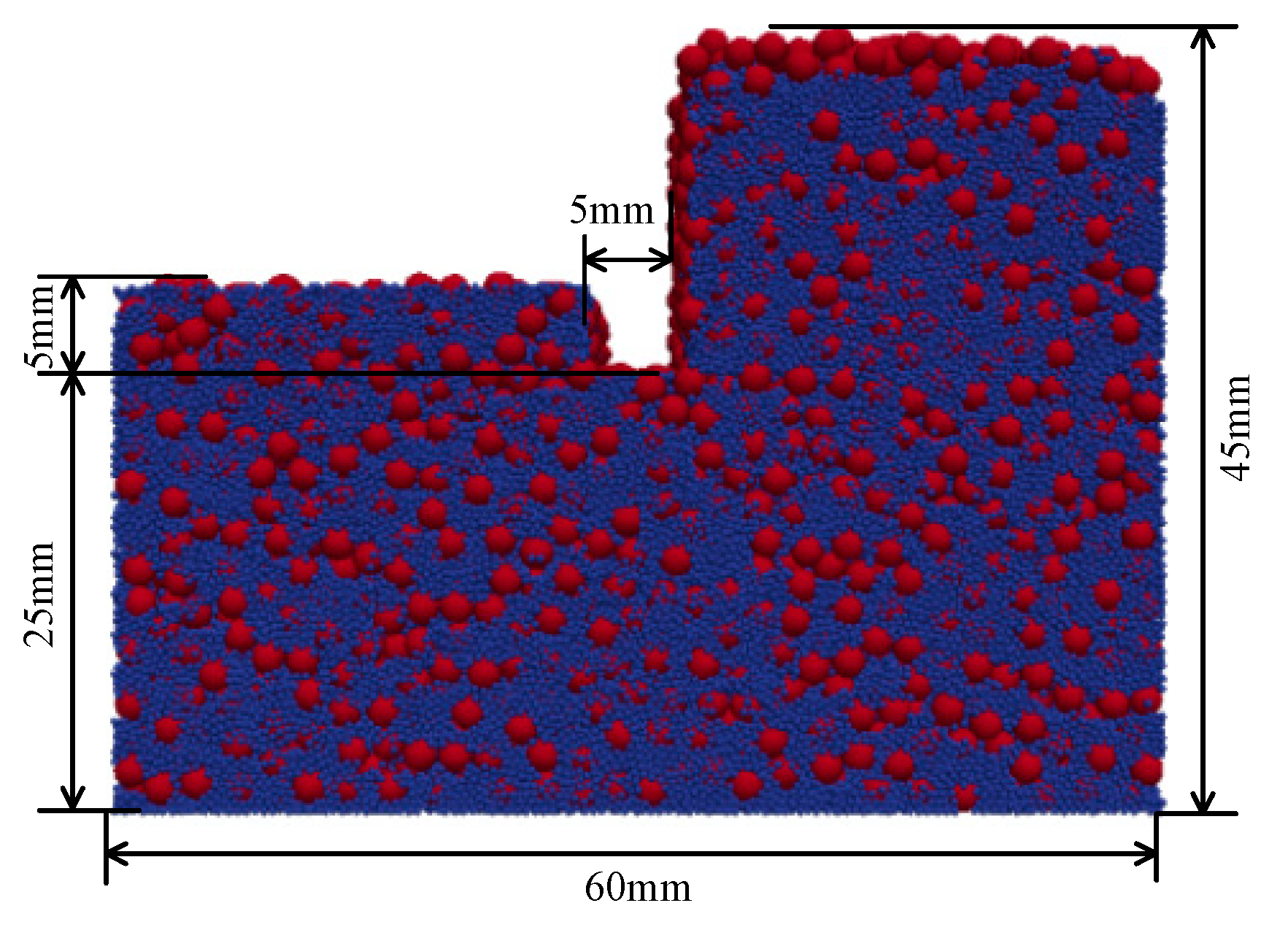
The solver developed for simulating the fluid phases was validated before performing the simulations. The literature shows that the piping phenomenon mainly occurs around the sheet piles. In this case, a narrow area is considered to reduce the computation effort, with the initial configuration displayed in Figure 1. The size of $L/d_{rw}$ is determined to be around 12, where $L$ is the sample scale in the $x$ direction and $d_{rw}$ denotes the diameter of the retaining wall. The dimension in the $y$ direction is the same as that in the $x$ direction. A retaining wall has $d_{wp}=0.025$ m, in which $d_{wp}$ refers to the distance above the bottom of the sand deposit. To mimic the excavation condition, the soil deposit was set to 0.03 and 0.045 m for the left and right side of the retaining wall, respectively, with a thickness of 0.06 m.

Spherical particles were adopted for the simulation using the Hertz contact model, with the properties of the materials presented in

Table 1. Properties of particles and boundary.

Young’s Modulus	Density of Particles	Radii of Particles	Friction Coefficient	Poission’s Ratio	Restitution Coefficient
5 MPa	2500 kg/m3	$r_{\min }=0.25 \mathrm{mm}$ $r_{\max }=1 \mathrm{mm}$	0.85	0.45	0.1

. For the erosion behavior, the impact of stiffness could be negligible [28], and it was thus reduced to 5MPa to reduce the computational effort. In the simulation process, the steps for data exchange between DEM and CFD were determined to be 10. Hence, the timesteps of DEM solver and CFD solver were set to $5\times {10}^{-6}$ and $5\times {10}^{-5}$ s, respectively. To better observe the seepage failure, we adopted binary-sized spheres for the simulations, with a mass ratio of 0.3 and 0.7 for the fine particles and coarse particles, respectively.

In the simulation, the numerical procedures involved two steps. First, we only used DEM software to prepare the soil skeleton. Particles were randomly generated and deposited into the container to achieve the quasi-static condition, followed by deleting the particles located in the region of the retaining wall for importing the boundary. After the sample preparation, we then submerged the area with fluid flow to perform the simulation.

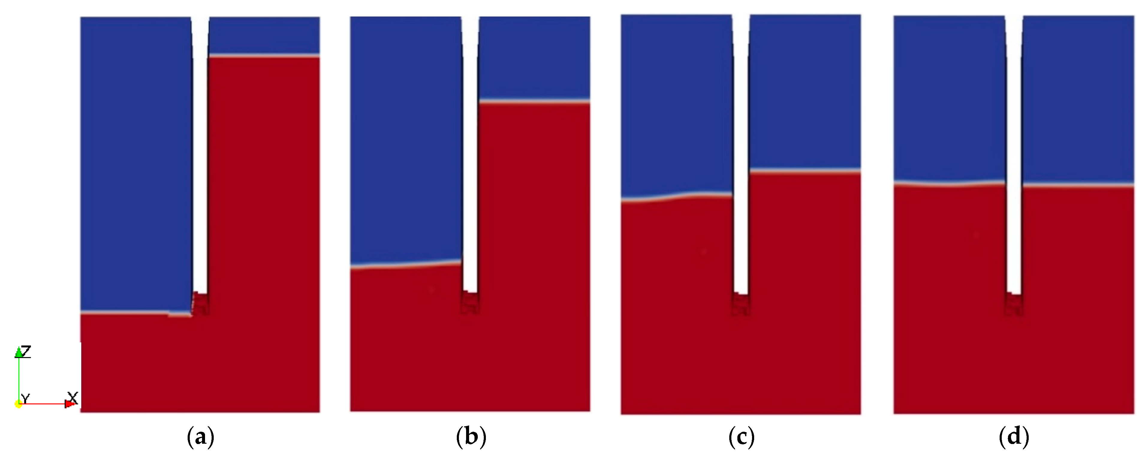
The hydraulic gradient was achieved with the definition of different water tables on different sides of the retaining wall. We identified the left side of the retaining wall as the downstream side for simulation and the upstream side as the right side of the retaining wall. Figure 2a depicts the initial conditions of the water table, with the blue and red colour indicating the air and water phases, respectively. For the simulation, the initial hydraulic gradient was set with the water table at 0.025 and 0.09 m for the downstream side and the upstream side, respectively. According to Figure 2, the fluid achieved a relatively static condition at t = 0.5 s.

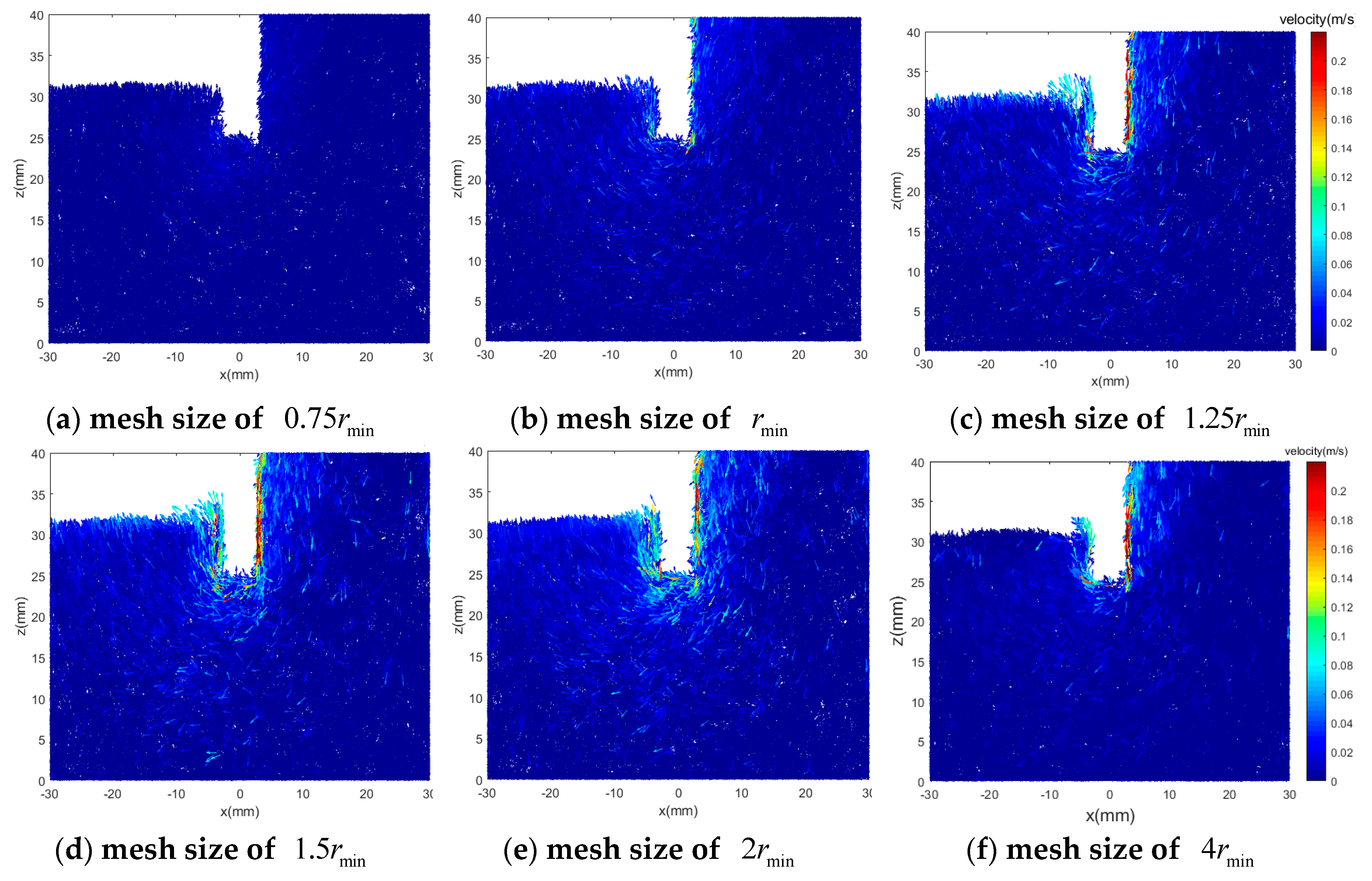
In the CFD approach, the boundary was subdivided into numerous cells to capture the fluid properties, and the dimension of the mesh cell is highly related to the velocity behavior in the literature [40,41]. Benmebarek et al. [41] conducted FEM simulations and found that the failure mechanism is difficult to capture using a coarse mesh. Hence, an approximate size must be selected for the meshes formed in the CFD boundary. Figure 3 depicts the velocity field using a different number of mesh elements at erosion initiation. The seepage impact induces the movement of particles with the high particle velocity concentrated near the wall for all the tests, particularly for the tests with a mesh size of $1.25r_{\min }$ and $1.5r_{\min }$.

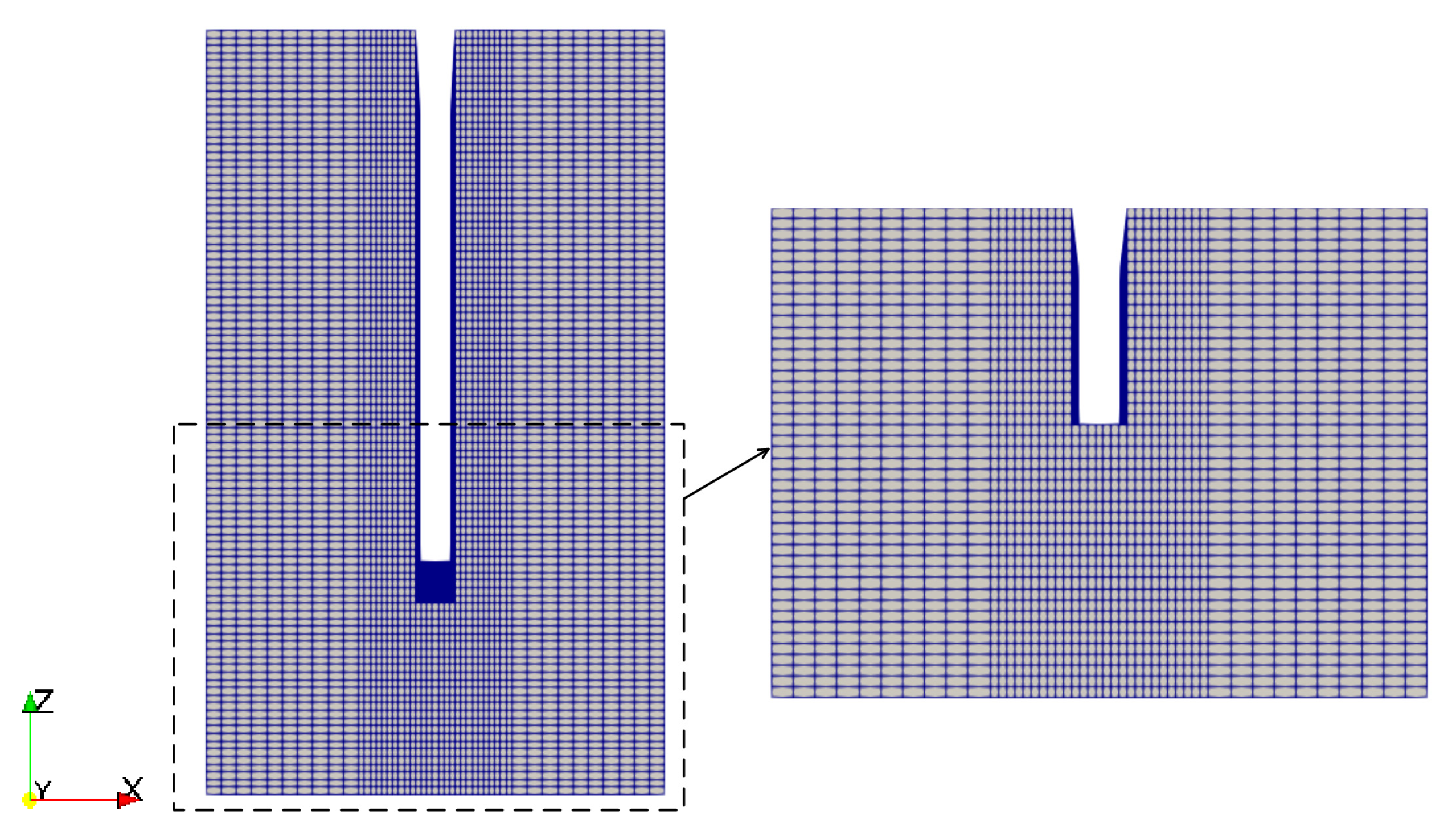
The results demonstrated that the developed technique can successfully simulate the seepage phenomenon with heave behavior, which mainly appears around the retaining wall. The refined meshes can more accurately capture the phenomenon. With an increasing number of mesh cells, the simulation time also increases. According to the theory of Terzaghi and Peck [42], the heave behavior for the lifting of the soil block occurs within the width of $D/2$, where $D$ refers to the embedment depth of the retaining wall. In such a case, to reduce the computation effort, the method adopts fine meshes with a size of $1.5r_{\min }$ in the central region within a span of $\left(-0.01,0.01\right)$ m in the $x$ direction. Regarding the other regions, the boundary is formed with coarse meshes. Figure 4 displays the meshes used in the simulations.

4. Observations of Seepage Failure

The water table for the downstream side was set to the same level as the bottom of the retaining wall. The impact of the hydraulic gradient was studied using different hydraulic heads $\left(h\right)$ in the upstream side. We selected five different $h$ values: 0.04, 0.05, 0.06, 0.07, 0.08 and 0.09 m, to perform the simulations. The process of seepage failure involves three stages: initial erosion, regressive erosion to form flow channels and the heave/boil phenomenon. We studied the peak position (in the z-direction) of particles located on the downstream side to represent the degree of boiling bulk. Figure 5 shows that no particles boil out when $h<0.06m$. The results indicated that the critical hydraulic condition appears at $h=0.06m$ for these gap-graded particles. The boiling phenomenon starts at $h\ge 0.06m$. The phenomenon of seepage failure increased with increasing h value.

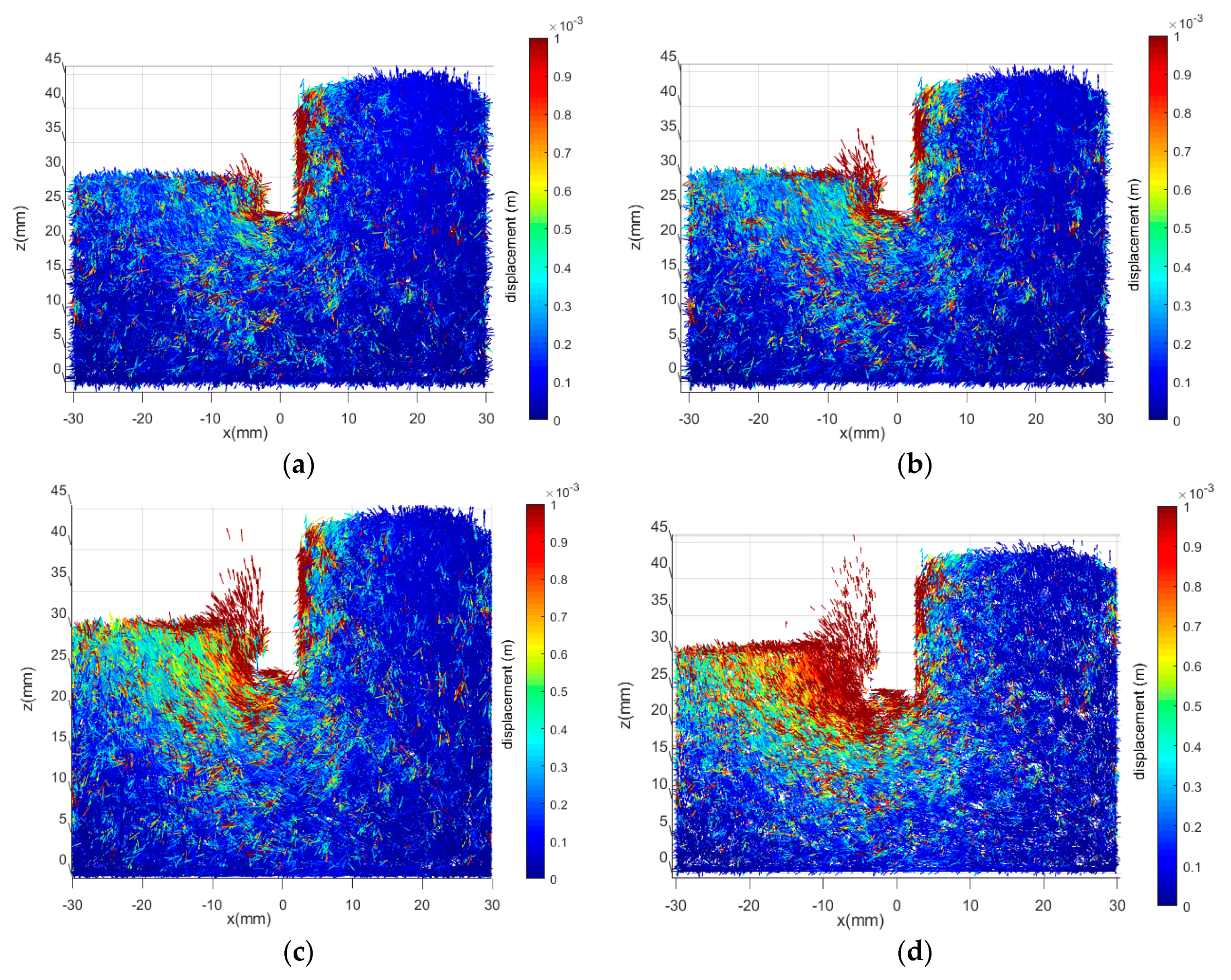
Figure 6 depicts the failure mechanism indicated by the displacement field with h ranging from 0.06 to 0.09 m at a simulation time of 0.5 s. The seepage impact induced larger displacements of particles with increasing water table, in particular for the downstream side. The results are consistent with Terzaghi and Peck’s theory as the heave phenomenon is concentrated near the wall. This demonstrates that the hydraulic gradient affects the shape of the failure mechanisms. Under a low hydraulic condition, we observed the boil bulk in a rectangular prism. When $h\ge 0.08m$, a triangular soil prism was obtained.

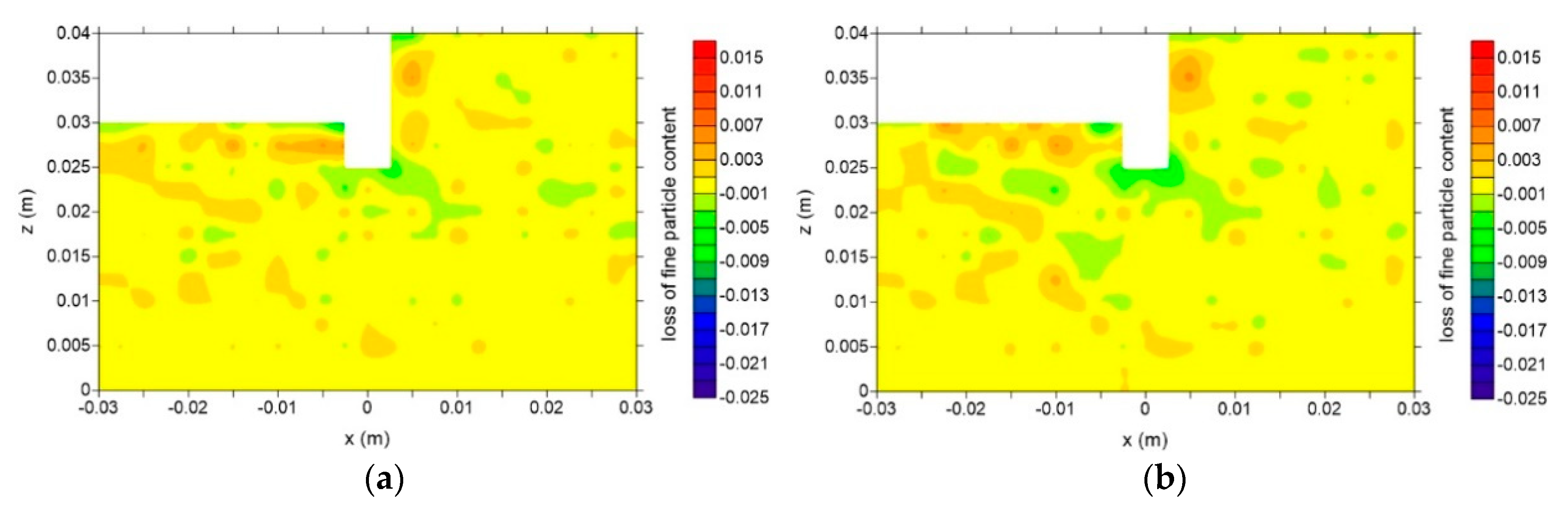
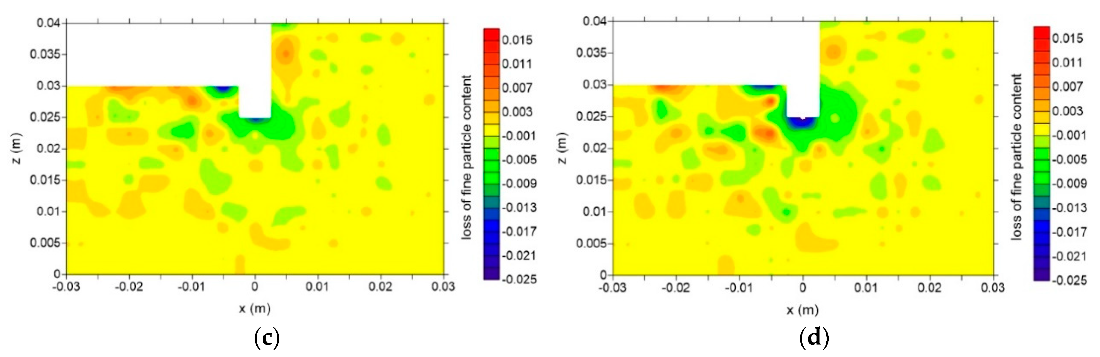
The initial erosion occurred with the detachment of fine particles inside the skeleton of coarse particles. In this case, we examined the erosion rate in terms of the loss of fine particles. Figure 7 depicts the lost fine particles inside the system during erosion under different hydraulic conditions. The results were estimated as the difference in fine particle content between t = 0.5 s and the initial stage. In the graphs, the negative values refer to the loss of fine particles and the positive values indicate an increased content of fine particles in local regions. The results were consistent with the behavior of the displacement field. The loss of fine particles mainly occurred around the retaining wall at the lower hydraulic condition; however, with increasing hydraulic head, it was widely distributed inside the skeleton. The results indicate that the seepage impact triggers the migration of fine particles and induces an increased content on the downstream side.

5. Micro-Scale Mechanisms of Seepage Failure and Discussion

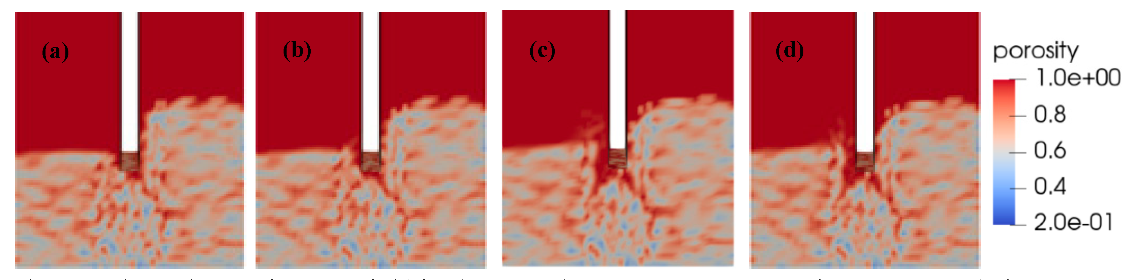
Section 4 showed that the seepage impact induces the rearrangement of particles, which alters the porosity of the system and affects the characteristics of the internal structure. Figure 8 and Figure 9 portray the evolution of mesh porosity during the erosion process under hydraulic heads of 0.06 and 0.09 m, respectively. Due to the lower magnitude of the embedment depth of the retaining wall, the change in porosity mainly occurred adjacent to the wall, particularly for h = 0.09 m. The results indicated that the fluid flow induces the movement of particles and produces a higher porosity on the downstream side near the boundary first. This would further trigger the detachment of particles located on the upstream side for the formation of the flow channel during erosion.

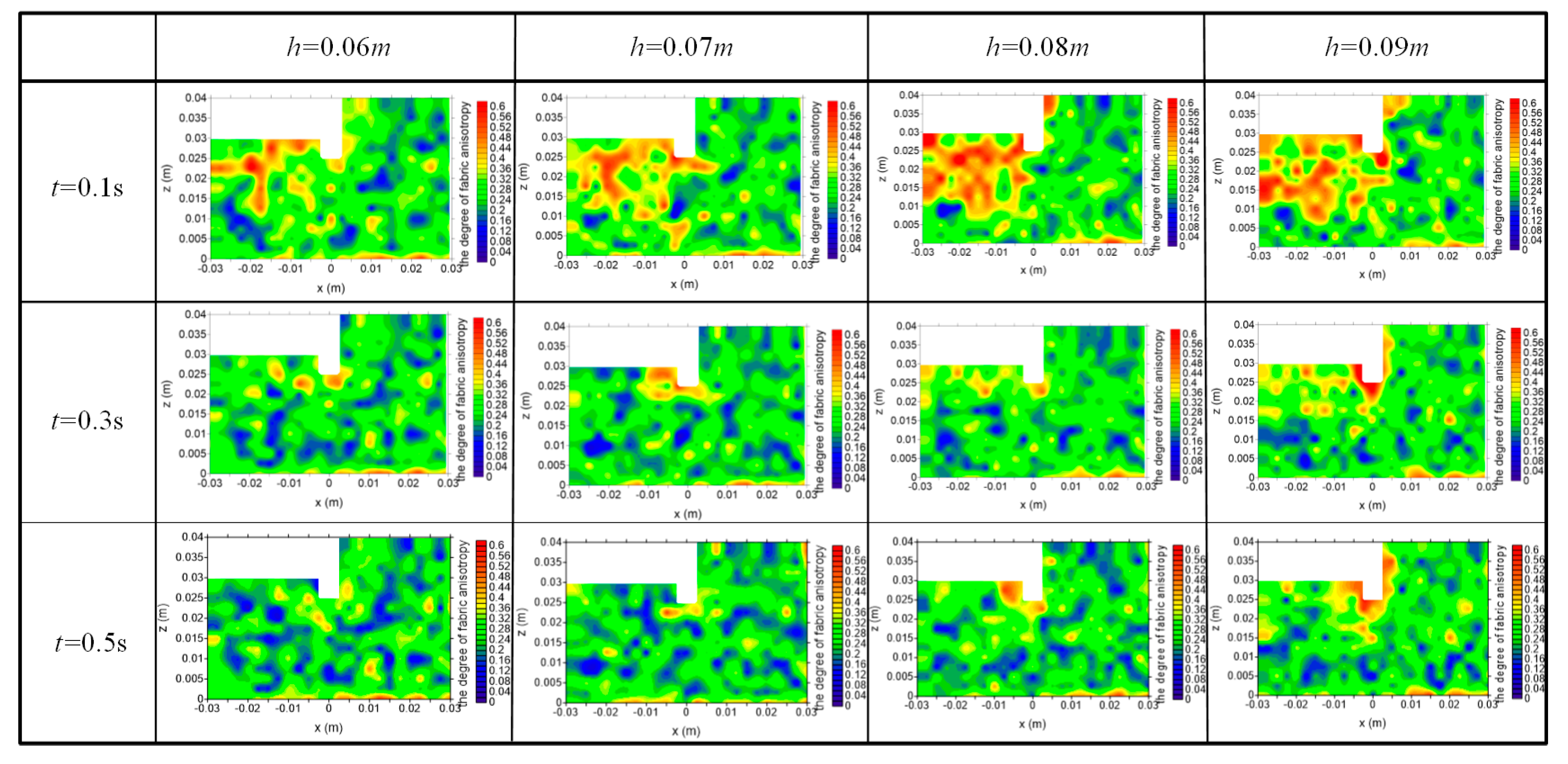
Fabric, which is the spatial arrangement of particles and associated voids, could provide insight into the anisotropy behavior of granular materials. Oda and Nakayama [43] introduced the fabric tensor to express the geometry made by discrete particles concretely. This tensor can thus be used to investigate the aspects of soil fabric at the particle-scale. Equation (11) gives the expression of the fabric tensor and the estimation of the degree of fabric anisotropy $\left(D_q\right)$ [44,45]:

$$\{\begin{array}{l}{\mathit{N}}_{ij}=\frac{1}{N_c}{\displaystyle \sum _{c=1}^{N_c}{\mathit{n}}_i^c{\mathit{n}}_j^c}\\ D_{ij}=\frac{15}{2}\left({\mathit{N}}_{ij}-\frac{1}{3}{\delta }_{ij}\right)\\ D_q=\sqrt{\frac{3}{2}{D}_{ij}{D}_{ji}}\end{array}$$

(11)

where ${\mathit{N}}_{ij}$ and $D_{ij}$ are the contact normal tensor and deviatoric part of the fabric tensor, respectively. ${\delta }_{ij}$ denotes the Kronecker delta. $N_c$ refers to the total number of contacts; and $\mathit{n}$ is the unit normal direction at the contact point c.

Figure 10 depicts the spatial distribution of fabric anisotropy during the process of erosion. The results portray the central plane, with a thickness of 10 mm, under different hydraulic conditions. The application of fluid flow increased the degree of fabric anisotropy, especially for the downstream side in the initial stage. After the formation of the flow channel, the area for the higher magnitudes of fabric anisotropy significantly reduced and was concentrated adjacent to the wall in the final collapse process. The results suggest that increases in particle velocity and particle displacement produce the structure under a more anisotropic condition, with the degree increasing alongside the hydraulic gradient during the erosion process.

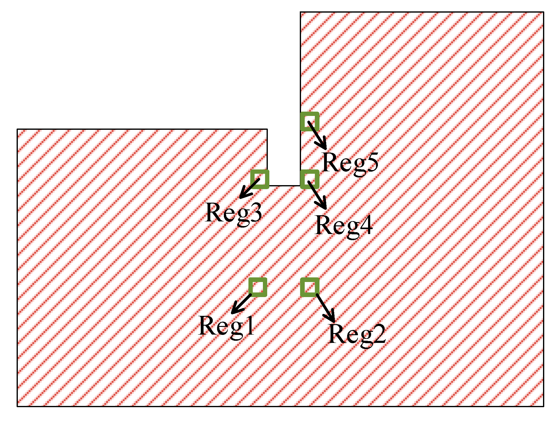
The results demonstrated that the fluid flow altered the distribution of voids and the internal structure. This would impact the field of the particle–fluid interaction force, which would further affect the overall response of granular materials on the macro-scale. We investigated the behavior of the drag force to better understand the erosion mechanisms. During erosion, the change in porosity field and fabric anisotropy mainly occurred around the boundary. Hence, we selected five local regions at the center of the system, located close to the retaining wall. The heights of the local regions were determined below, on the same level as and above the wall for the downstream and upstream sides. Figure 11 displays the distribution of the regions inside the system.

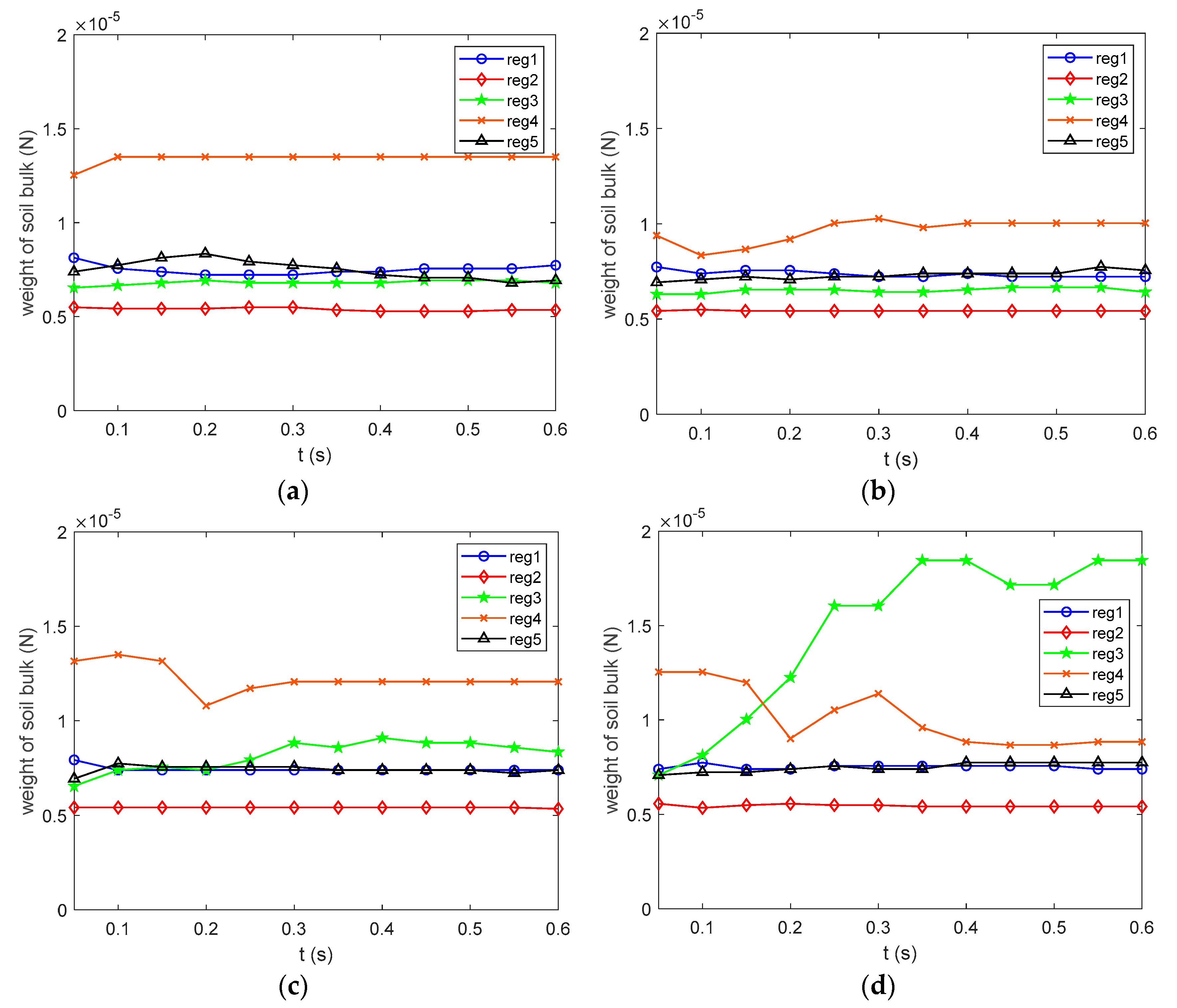
Figure 12 displays the bulk soil weight for each local region. The soil located below the wall on the upstream side almost maintained constant for each hydraulic gradient. At h = 0.06 m, due to the lower hydraulic condition, the influence on the weight was relatively small during erosion. The initial seepage impact induced a loss of soil weight in region reg1, but the magnitude increased for regions reg3 and reg4. With increasing water head, the main alteration was observed in the area adjacent to the boundary (regions reg3 and reg4 in the graphs). The results indicated that the initial erosion started with particles located below the retaining wall on the downstream side, which lifted upwards and concentrated near the boundary during erosion, in particular for the larger hydraulic gradient. The impact regressed to the upstream side and produce a decrease in the weight in the region close to the boundary. The continuous fluid flow transported particles located at a higher height from the upstream side to the downstream side to produce seepage failure.

The movement of particles started as the seepage velocity reached the critical value, which is strongly related to the magnitude of the drag force. The heave/boiling behavior occurred as the drag force $\left(F_d\right)$ exceeded the gravity of the soil bulk $\left(W\right)$. In this case, Figure 13 shows the evolution of the $\raisebox{1ex}{$F_d$}\!\left/ \!\raisebox{-1ex}{$W$}\right.$ ratio to further understand the erosion mechanism. Similar to the behavior of soil weight, the region near the boundary contained a higher magnitude of the ratio, in comparison with the other local regions, to trigger the detachment of particles. This showed a higher hydraulic head induced a larger ratio in the initial stage for each local region, with the peak magnitude obtained in the region reg3. Due to the reduction in fluid velocity, the value continuously decreased as the flow approached the steady state. Based on the graphs, we inferred that boiling failure occurred as $\raisebox{1ex}{$F_d$}\!\left/ \!\raisebox{-1ex}{$W$}\right.\ge 1$ for the region close to the wall on the downstream side.

6. Conclusions

This paper illustrates a CFD–DEM simulation of hydraulic heave behavior subjected to seepage impact, outlining the continuum-particle dual scale observations on the phenomenon. The results demonstrated that seepage failure mainly occurs with the detachment of fine particles through the soil skeleton. The loss of fine particle content was studied to understand the erosion rate under different hydraulic conditions, which mainly concentrated around the sheet pile at the lower hydraulic condition. The influenced region developed with the increasing hydraulic gradient. To better understand the erosion mechanism, we investigated the temporal–spatial distribution of porosity and the internal structure of the system. The results indicated that the seepage impact induces a loose condition for the region concentrated around the wall and produces an increase in the fabric anisotropy for the region, with the severe loss of fine particles. Combined with the results of drag force, we inferred that the seepage erosion highly depends on the behavior of the drag force located adjacent to the retaining wall on the downstream side. The heave behavior occurs when the drag force in this region is larger than the corresponding weight of the bulk soil. This causes the detachment of particles and regression to the upstream side, forming flow channels and exacerbating the erosion failure, which further alters the characteristics of the internal structure.

References

- Sterpi, D. Effects of the erosion and transport of fine particles due to seepage flow. Int. J. Geomech. 2003, 3, 111–122. [Google Scholar] [CrossRef]
- Richards, K.S.; Reddy, K.R. Critical appraisal of piping phenomena in earth dams. Bull. Eng. Geol. Environ. 2007, 66, 381–402. [Google Scholar] [CrossRef]
- Arulanandan, K.; Perry, E.B. Erosion in relation to filter design criteria in earth dams. J. Geotech. Eng. 1983, 109. [Google Scholar] [CrossRef]
- Shaikh, A.; Ruff, J.F.; Abt, S.R. Erosion rate of compacted Na-Montmorillonite soils. J. Geotech. Eng. 1988, 114. [Google Scholar] [CrossRef]
- Sharif, Y.A.; Elkholy, M.; Hanif Chaudhry, M.; Imran, J. Experimental Study on the Piping Erosion Process in Earthen Embankments. J. Hydraul. Eng. 2015, 141. [Google Scholar] [CrossRef]
- Moore, W.L.; Masch, F.D. Experiments on the scour resistance of cohesive sediments. J. Geophys. Res. 1962, 67, 1437–1446. [Google Scholar] [CrossRef]
- Chapuis, R.P. Quantitative measurement of the scour resistance of natural solid clays. Can. Geotech. J. 1986, 23, 132–141. [Google Scholar] [CrossRef]
- Chapuis, R.P.; Gatien, T. An improved rotating cylinder technique for quantitative measurements of the scour resistance of clays. Can. Geotech. J. 1986, 23, 83–87. [Google Scholar] [CrossRef]
- Chang, D.S.; Zhang, L.M. Critical Hydraulic Gradients of Internal Erosion under Complex Stress States. J. Geotech. Geoenviron. Eng. 2013, 139, 1454–1467. [Google Scholar] [CrossRef]
- Reddi, L.N.; Lee, I.; Bonala, M. Comparison of internal and surface erosion using flow pump tests on a sand-kaolinite mixture. Geotech. Test. J. 2000, 23, 116–122. [Google Scholar]
- Wan, C.F.; Fell, R. Investigation of rate of erosion of soils in embankment dam. J. Geotech. Geoenviron. Eng. 2004, 130, 373–380. [Google Scholar] [CrossRef]
- Hanson, G.J. Development of a jet index to characterize erosion resistance of soils in earthen spillways. Trans. ASAE 1991, 34, 2015–2020. [Google Scholar] [CrossRef]
- Tomlinson, S.S.; Vaid, Y.P. Seepage forces and confining pressure effects on piping erosion. Can. Geotech. J. 2000, 37, 1–13. [Google Scholar] [CrossRef]
- Bendahmane, F.; Marot, D.; Rosquoët, F.; Alexis, A. Characterization of internal erosion in sand kaolin soils. Revue Européenne de Génie Civil 2011, 10, 505–520. [Google Scholar] [CrossRef]
- Sato, M.; Kuwano, R. Laboratory testing for evaluation of the influence of a small degree of internal erosion on deformation and stiffness. Soils Found. 2018, 58, 547–562. [Google Scholar] [CrossRef]
- Xie, Q.; Liu, J.; Han, B.; Li, H.; Li, Y.; Li, X. Critical Hydraulic Gradient of Internal Erosion at the Soil–Structure Interface. Processes 2018, 6, 92. [Google Scholar] [CrossRef] [Green Version]
- Foster, M.; Fell, R.; Spannagle, M. The statistics of embankment dam failures and accidents. Can. Geotech. J. 2000, 37, 1000–1024. [Google Scholar] [CrossRef]
- Tanaka, T.; Verruijt, A. Seepage Failure of Sand behind Sheet Piles. The Mechanism and Practical Approach to Analyze. Soils Found. 1999, 39, 27–35. [Google Scholar] [CrossRef] [Green Version]
- Moffat, R.; Fannin, R.J.; Garner, S.J. Spatial and temporal progression of internal erosion in cohesionless soil. Can. Geotech. J. 2011, 48, 399–412. [Google Scholar] [CrossRef]
- Luo, Y.; Nie, M.; Xiao, M. Flume-scale experiments on suffusion at bottom of cutoff wall in sandy gravel alluvium. Can. Geotech. J. 2017, 54, 1716–1727. [Google Scholar] [CrossRef] [Green Version]
- Wang, S.; Chen, J.; Sheng, J.; Luo, Y. Laboratory investigation of stress state and grain composition affecting internal erosion in soils containing a suspended cut-off wall. KSCE J. Civ. Eng. 2015, 20, 1283–1293. [Google Scholar] [CrossRef]
- Fleshman, M.S.; Rice, J.D. Laboratory Modeling of the Mechanisms of Piping Erosion Initiation. J. Geotech. Geoenviron. Eng. 2014, 140. [Google Scholar] [CrossRef]
- Kawano, K.; O’Sullivan, C.; Shire, T. Using DEM to assess the influence of stress and fabric inhomogeneity and anisotropy on susceptibility to suffusion. In Proceedings of the ICSE 2016 (8th International Conference on Scour and Erosion), Oxford, UK, 12–15 September 2016. [Google Scholar]
- Shire, T.; O’Sullivan, C.; Hanley, K.J.; Fannin, R.J. Fabric and Effective Stress Distribution in Internally Unstable Soils. J. Geotech. Geoenviron. Eng. 2014, 140. [Google Scholar] [CrossRef] [Green Version]
- Yerro, A.; Rohe, A.; Soga, K. Modelling Internal Erosion with the Material Point Method. Procedia Eng. 2017, 175, 365–372. [Google Scholar] [CrossRef]
- Chen, S.Y.; Doolen, G.D. Lattice boltzmann method for fluid flows. Annu. Rev. Fluid Mech. 1998, 30, 329–364. [Google Scholar] [CrossRef] [Green Version]
- Zhou, Y.; Shi, Z.; Zhang, Q.; Jang, B.; Wu, C. Damming process and characteristics of landslide-debris avalanches. Soil Dyn. Earthq. Eng. 2019, 121, 252–261. [Google Scholar] [CrossRef]
- El Shamy, U.; Denissen, C. Microscale characterization of energy dissipation mechanisms in liquefiable granular soils. Comput. Geotech. 2010, 37, 846–857. [Google Scholar] [CrossRef]
- Schmeeckle, M.W. The role of velocity, pressure, and bed stress fluctuations in bed load transport over bed forms: Numerical simulation downstream of a backward-facing step. Earth Surf. Dyn. 2015, 3, 105–112. [Google Scholar] [CrossRef] [Green Version]
- Cui, X.; Li, J.; Chan, A.; Chapman, D. Coupled DEM–LBM simulation of internal fluidisation induced by a leaking pipe. Powder Technol. 2014, 254, 299–306. [Google Scholar] [CrossRef]
- Kawano, K.; Shire, T.; O’Sullivan, C.; Nezamabadi, S.; Luding, S.; Delenne, J.Y. Coupled DEM-CFD Analysis of the Initiation of Internal Instability in a Gap-Graded Granular Embankment Filter. EPJ Web Conf. 2017, 140, 10005. [Google Scholar] [CrossRef] [Green Version]
- Tao, H.; Tao, J. Quantitative analysis of piping erosion micro-mechanisms with coupled CFD and DEM method. Acta Geotech. 2017, 12, 573–592. [Google Scholar] [CrossRef]
- LIGGGHTS. LIGGGHTS (R)-Public Documentation, Version 3.X. Available online: http://www.cfdem.com (accessed on 18 February 2015).
- OpenFOAM. OpenFOAM—The Open Source CFD Toolbox. The OpenFOAM Foundation. 2015. Available online: http://www.openfoam.org (accessed on 22 May 2015).
- Jasak, H. Error Analysis and Estimation for the Finite Volume Method with Applications to Fluid Flows. Ph.D. Thesis, Imperial College, London, UK, 1996. [Google Scholar]
- Cundall, P.A.; Strack, O. A discrete numerical model for granular assemblies. Geotechnique 1979, 29, 47–65. [Google Scholar] [CrossRef]
- Di Felice, R. The voidage function for fluid-particle interaction systems. Int. J. Multiph. Flow 1994, 20, 153–159. [Google Scholar] [CrossRef]
- Goniva, C.; Blais, B.; Radl, S.; Kloss, C. Open source CFD-DEM modelling for particle-based processes. In Proceedings of the Eleventh International Conference on CFD in the Minerals and Process Industries, CSIRO, Melbourne, Australia, 7–9 December 2015. [Google Scholar]
- Kloss, C.; Goniva, C.; Aichinger, G.; Pirker, S. Comprehensive DEM-DPM-CFD simulations-Model synthesis, experimental alidation and scalability. In Proceedings of the Seventh International Conference on CFD in the Minerals and Process Industries, CSIRO, Melbourne, Australia, 9–11 December 2009. [Google Scholar]
- Sande, P.C.; Ray, S. Mesh size effect on CFD simulation of gas-fluidized Geldart A particles. Powder Technol. 2014, 264, 43–53. [Google Scholar] [CrossRef]
- Benmebarek, N.; Benmebarek, S.; Kastner, R. Numerical studies of seepage failure of sand within a cofferdam. Comput. Geotech. 2005, 32, 264–273. [Google Scholar] [CrossRef]
- Terzaghi, K.; Peck, R.B. Soil Mechanics in Engineering; John Wiley & Sons: New York, NY, USA, 1948. [Google Scholar]
- Oda, M.; Nakayama, H. Yield function for soil with anisotropic fabric. J. Eng. Mech. 1989, 115, 89–104. [Google Scholar] [CrossRef]
- Bathurst, R.J.; Rothenburg, L. Observations on stress-force-fabric relationships in idealized granular materials. Mech. Mater. 1990, 9, 65–80. [Google Scholar] [CrossRef]
- Li, X.; Yu, H.-S. On the stress-force-fabric relationship for granular materials. Int. J. Solids Struct. 2013, 50, 1285–1302. [Google Scholar] [CrossRef]
Figure 1.
The initial configuration for the numerical simulation.
Figure 2.
The evolution of fluid phases during simulation at t = (a) 0.0, (b) 0.1, (c) 0.3 and (d) 0.5 s.
Figure 3.
The impact of mesh size on the observation of erosion at t= 0.1s.
Figure 4.
The meshes used in the computational fluid dynamics (CFD) boundary.
Figure 5.
The evolution of achieved peak position in the downstream side at different water tables.
Figure 6.
Displacement field at t = 0.5 s for h = (a) 0.06, (b) 0.07, (c) 0.08 and (d) 0.09 m.
Figure 7.
The loss of fine particle content at t = 0.5 s for h = (a) 0.06, (b) 0.07, (c) 0.08 and (d) 0.09 m.
Figure 8.
The evolution of porosity field for the test with h = 0.06 m at t= (a) 0.0, (b) 0.1, (c) 0.3 and (d) 0.5 s.
Figure 9.
The evolution of porosity field for the test with h = 0.09 m at t = (a) 0.0, (b) 0.1, (c) 0.3 and (d) 0.5 s.
Figure 10.
The temporal–spatial distribution of fabric anisotropy under different water tables.
Figure 11.
The illustration of defined local regions inside the system.
Figure 12.
The behavior of soil weight at different local regions during erosion for h = (a) 0.06, (b) 0.07, (c) 0.08 and (d) 0.09 m.
Figure 13.
The behavior for the ratio of at different local regions for h = (a) 0.06, (b) 0.07, (c) 0.08 and (d) 0.09 m.