Article

Development of a Hydrological Boundary Method for the River–Lake Transition Zone Based on Flow Velocity Gradients, and Case Study of Baiyangdian Lake Transition Zones, China

1
State Key Laboratory of Water Environment Simulation, Beijing Normal University, Beijing 100875, China
2
Key Laboratory for Water and Sediment Sciences of Ministry of Education, Beijing Normal University, Beijing 100875, China
*
Author to whom correspondence should be addressed.
Water 2020, 12(3), 674; https://doi.org/10.3390/w12030674
Submission received: 30 January 2020 / Revised: 24 February 2020 / Accepted: 26 February 2020 / Published: 1 March 2020
(This article belongs to the Section Hydraulics and Hydrodynamics)

Abstract

:
The river–lake transition zone is affected by many environmental factors, leading to significant dynamics and complexity. This makes the boundary unclear, and not enough attention has been paid to this problem by scholars, even though it has great significance for research on water quantity, water quality, and the aquatic environment. In this paper, we define this transition zone, define its upper and lower boundaries, and develop the method for defining the hydrologic boundary. It includes a method for defining the upper boundary, based on the flow velocity mutation point, and a method for defining the lower boundary, based on the velocity gradient field. We then used this approach to examine the transition zones between the Fu River, Baigou Canal, and Baiyangdian Lake in China as a case study. We found that the upper boundary of the Fu River–Baiyangdian Lake transition zone was 2.35 km upstream of the lake’s inlet; the lower boundary was farthest from the lake’s inlet in July, and the maximum area of the transition zone was 2.603 km2. The lower boundary was closest to the lake’s inlet in March, when the minimum area was 1.598 km2. The upper boundary of the Baigou Canal–Baiyangdian Lake transition zone was 2.18 km upstream from the lake inlet, and the lower boundary was farthest from the lake’s inlet in August, when the maximum area was 2.762 km2. The lower boundary was closest to the lake’s inlet in April, when the minimum area was 0.901 km2.

1. Introduction

An ecotone represents the transition zone between adjacent ecological systems, and has characteristics that are uniquely defined by the spatial and temporal scales of the adjacent ecological systems, and by the strength of the interactions between them [1]. This concept is mostly used by terrestrial ecologists, but the concept can be applied to any border or transitional zone between adjacent ecological systems [2]. Lakes and rivers are important aquatic components of an ecosystem, and are intimately connected in an alternating series of lentic and lotic reaches in many regions. The river–lake transition zone that occurs between a stream and a lake also constitutes an ecotone [3]. This zone represents the transition from a relatively shallow habitat in a fast-flowing body of water to a relatively deep habitat in slow-flowing water [4]. The zone has a longitudinal gradient of environmental factors, such as the current velocity, turbidity, nutrient concentrations, and photosynthetic productivity [5,6]. The transitions between aquatic species assemblages are pronounced in this transition zone [7]. This is because the ecotone characteristics also determine the biotic composition of an ecosystem [8,9], and therefore, play an important role in the development and evolution of aquatic ecosystems. The transition zone also provides migratory pathways for aquatic and other organisms, and satisfies the ecological water requirements of the river and lake [10,11], and represents a key area for gathering and exchanging nutrients [12,13]. Due to the high density of particulate matter, which supplies vital sources of energy and nutrients in the water’s flow, the zone represents a habitat for many aquatic species, including both macro- and micro-fauna and macro- and micro-flora [14,15,16].
Researchers have carried out important work on the hydrodynamics, water quality, and biological characteristics in the transition zone, especially near the inlets and outlets of lakes [17]. The transition zone is where the river interacts directly with the lake, and it is affected by factors, such as runoff, tides, waves, coastal currents, and winds, leading to complex hydrodynamic conditions [18]. In the transition zone, water evolves from a lotic to a lentic environment, which represents a change from fast-flowing to slow-flowing water [9]. This creates an obvious current velocity gradient [5]. The water’s hydrodynamic characteristics are mainly controlled by factors such as the depth and width of the river and the initial velocity of the river water when it enters the transition zone, which can be described using hydrodynamic stream theory [19]. The transition zone mixes flows from the river and lake systems that have different physical and chemical properties, leading to the deposition of organic matter and the development of a gradient of mixing conditions [20]. The river flow causes the accumulation of pollutants at the lake’s inlet, and pollution is more serious than at the lake’s center [21,22]. The transition zones have higher biodiversity and population density compared with values in the adjacent rivers and lakes, but these effects can vary in response to changes in the hydrodynamic conditions and landform characteristics [17]. Timms [23] analyzed data from Lake Wyara from 1987 to 1999, and found that the number of invertebrate species was larger in the transition zones than in the lake. Moore and Hendry [24] and Sharpe et al. [25] found that the number and size of a fish species, the three-spined spine stickleback, were significantly larger at the inlet of Misty Lake than in adjacent rivers and lakes. In aquatic ecosystems, flow rate is often the key factor that affects the biotic composition [26,27]. The differences in species of aquatic organisms, and their populations, depend mainly, but not exclusively, on the strength of the current [28].
The above research results demonstrate that the transition zone plays an important role in the ecological water supply and in maintenance of the biodiversity of aquatic ecosystems. Despite this importance, little effort has been focused on transition zones [17], and in particular, insufficient attention has been paid to defining their boundaries. To improve research on transition zones, it will be necessary to clarify the boundaries of these zones. Defining the hydrological boundary of the transition zone clarifies the scope and lays the foundation for the research on various aspects of water quality, water quantity, and aquatic environment. As the key link of water supply, water quality guarantee and aquatic environment maintenance, defining a hydrological boundary has provided scientific support in many aspects, such as water quality improvement, biodiversity maintenance and aquatic environmental protection. Pritchard [29] proposed a method for defining estuary boundaries based on water salinity gradients. Li et al. [30] further developed and perfected this approach for estuaries, and proposed a method to define the boundaries of the near-estuary section, the estuary section, and the offshore section that lies outside the estuary. Because the salinity difference between freshwater and seawater in an estuary is obvious, the zone where freshwater and saltwater are exchanged can be accurately identified [31]. However, the effects of waves, tides, and other hydrodynamic factors lead to a constantly changing transition zone, which is more difficult to account for in practical management of these ecosystems [32].
Freshwater systems may be more difficult to analyze, because we do not yet know whether any factor differs as clearly as the salinity in saltwater ecosystems. Wang et al. [33] proposed a dynamic definition method for the tail-reach of an inflowing river, which was based on the hydrodynamic relationship between the inflowing river and the lake it flows into during both, the wet season and the dry season. This method can reflect the hydrodynamic characteristics of the tail-reach river and, based on the measured hydrological data, can help to define boundaries that are consistent with the actual range [34]. However, for a river–lake transition zone, this method only defines the boundary of the upstream river section, and our literature review found no method for defining the boundary for the downstream boundary of the transition zone. In recent years, some scholars have used remote sensing technology to monitor changes in the transition zones and lake inlets [35,36]. This research can let researchers quantify the boundary changes over many years and clarify their evolution. However, it requires a large amount of data and has limited application scope, as the approach is more suitable for the boundary between water and land, which is clearly visible and which shows clear dynamic changes [37].
The current state of research on transition zones inspired us to perform the present study. Hydrodynamic conditions, and especially flow velocity gradients, are obvious characteristics of such zones, and directly affect the transitions and changes of water quality, biological characteristics, and many other aspects of the transition zone. To objectively define the boundaries of the transition zone, we hypothesized that one promising approach would be to study the associated velocity gradient. We had four specific research goals: First, to define the boundary positions within the transition zone; second, to develop a boundary definition process for the different boundary types; third, to develop a method for defining the boundaries based on the velocity gradient; and fourth, to confirm the objectivity and feasibility of the proposed method using a case study.

2. Development of a Hydrological Boundary Method for a River–Lake Transition Zone

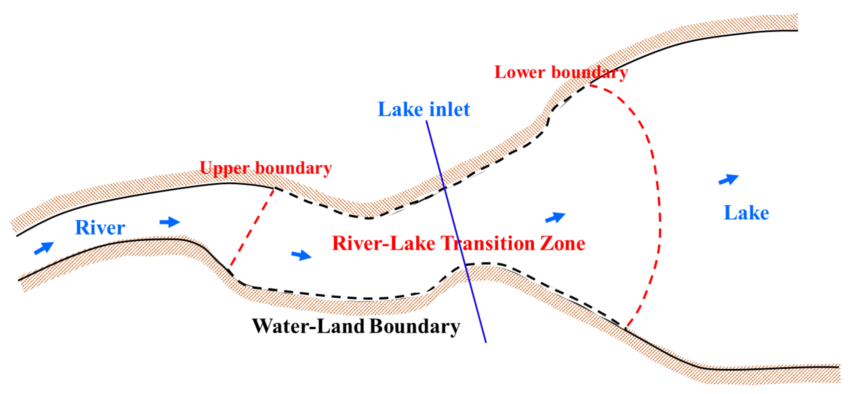
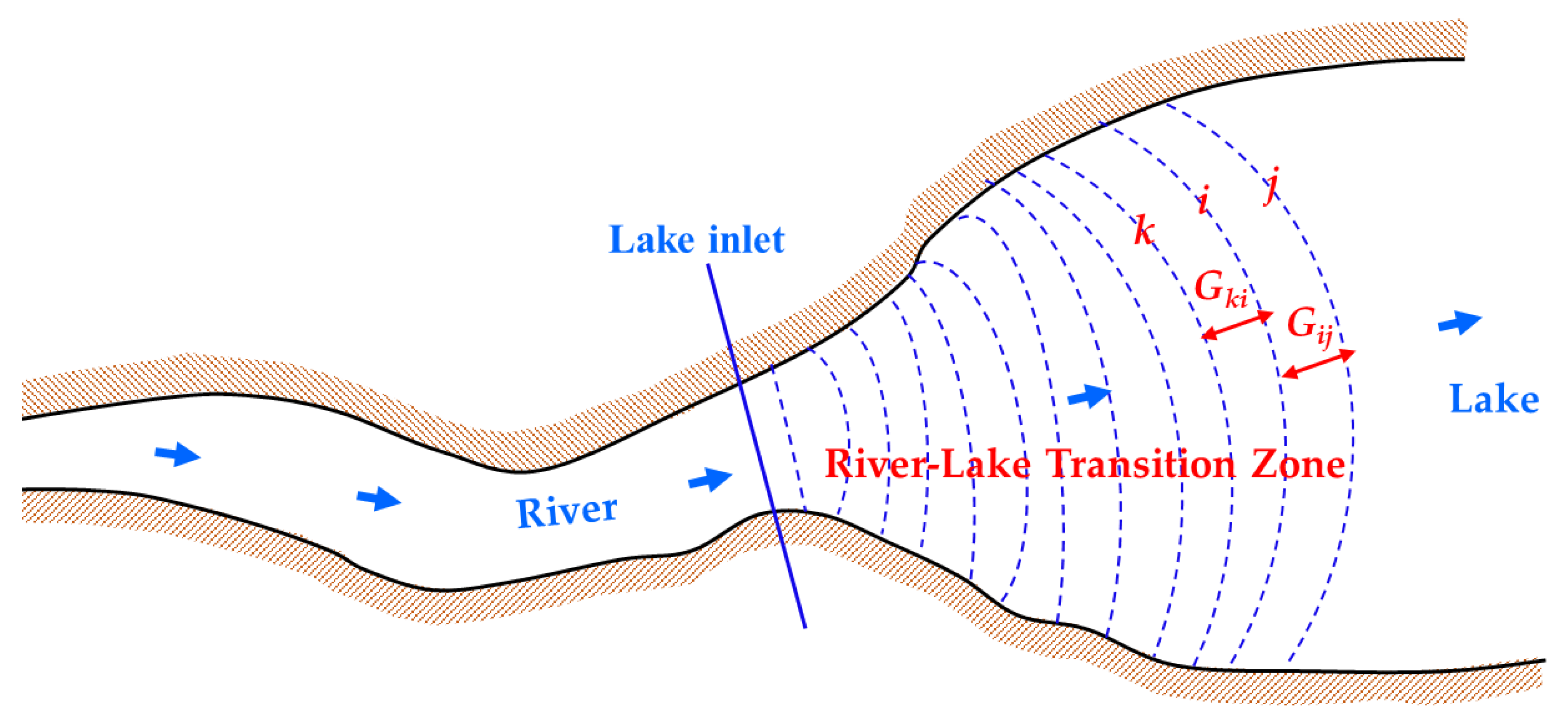
2.1. Definition of the Transition Zone

Table 1 summarizes the results of our literature review to identify definitions of the transition zone and the boundaries of the transition zone between a river and the lake that it flows into.
Based on these previous definitions, we define the river–lake transition zone as the interface between the river and lake, where a water velocity gradient develops, and has a relatively complex structure, which is formed by exchanges and interactions among water volumes, nutrients, and aquatic organisms.

2.2. Types of Boundaries in the Transition Zone

Based on the spatial location of the transition zone, and its morphological and hydrodynamic characteristics, we can define two types of boundaries. The first type is the water–land boundary, where the water body meets the land. Examples include natural riverbanks and lakeshores, and artificial embankments. Such boundaries can be identified by interpretation of remote sensing images and by field surveys based on information such as topographic and elevation data. The second type is the hydrological boundary between bodies of water, and can be further divided into upper and lower boundaries that correspond to the upstream and downstream directions, respectively, of the water flow where it enters the lake (Figure 1). In this paper, we defined the lake’s inlet as the position between the river and lake where the width of the channel (thus, of the water surface) increases continuously as water enters the lake.

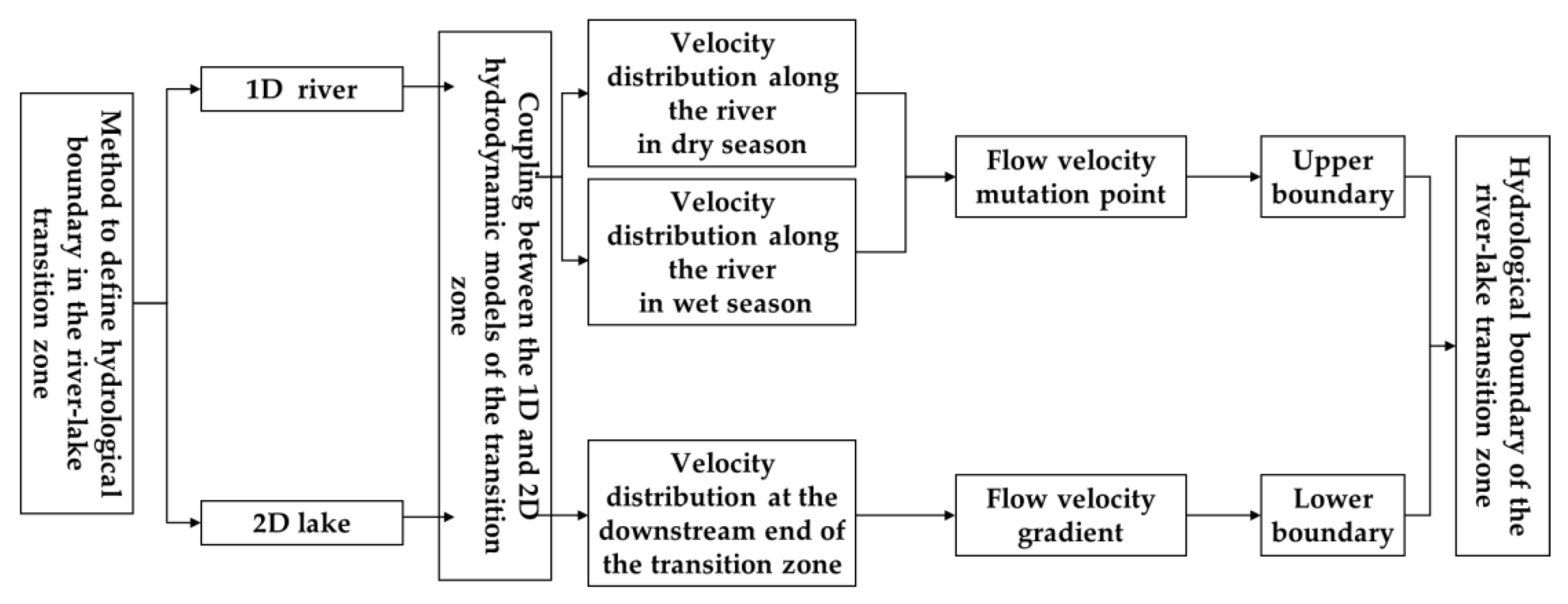
2.3. Defining Hydrological Boundaries in the River–Lake Transition Zone

2.3.1. Process

Researchers have developed one-dimensional (1D) [38] and two-dimensional (2D) [39] hydrodynamic models of the transition zone. 1D models describe flow that occurs primarily along a single axis, and are, therefore, suitable for rivers, which are linear features. In contrast, 2D models can account for flows along two axes, and are, therefore, more suitable for lakes (See Section 3.2 for details of the models we used). We combined these models to simulate the distribution of flow velocities in the transition zone and used this distribution to clarify the hydrodynamic processes. Based on the variation in the flow velocity, we established a functional relationship between the flow velocity and the distance along the river (measured from the lake’s inlet) during the wet and dry seasons. During the dry season or a season with normal water availability, the flow velocity of the river changes little, showing a small fluctuation around a mean flow velocity. During the wet season, the flow can change dramatically. We fitted a functional equation that describes the relationship between the flow velocity and the distance using the velocity and distance from the inlet in the simulation. We used polynomial curve fitting, and used the flow velocity mutation point created by the jacking force (where the higher lake level impedes the flow of water into the river, thus, affecting the flow velocity of the river) in the dry and wet seasons to represent the upper boundary of the transition zone (defined in more detail in Section 2.3.2). Based on the distribution of flow velocities in the lake, we calculated the flow velocity gradient within the transition zone between the outermost velocity lines, which is between the minimum velocity lines. We then identified the lower boundary based on these lines and defined the flow velocity gradient at this boundary to define the end of the transition zone (defined in more detail in Section 2.3.3). Figure 2 summarizes the process of defining the hydrological boundary.

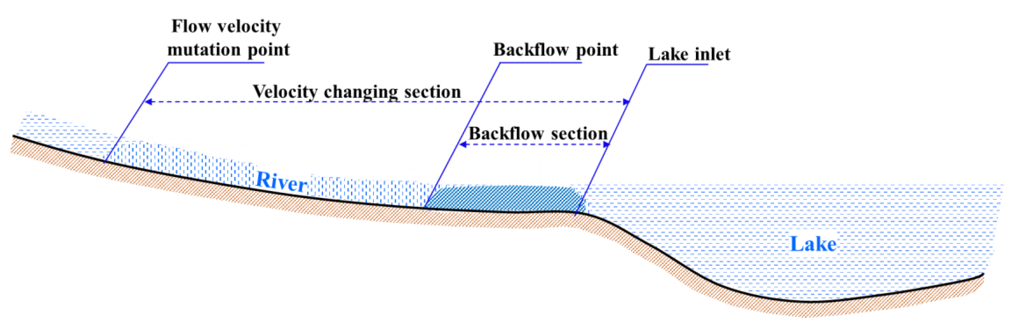
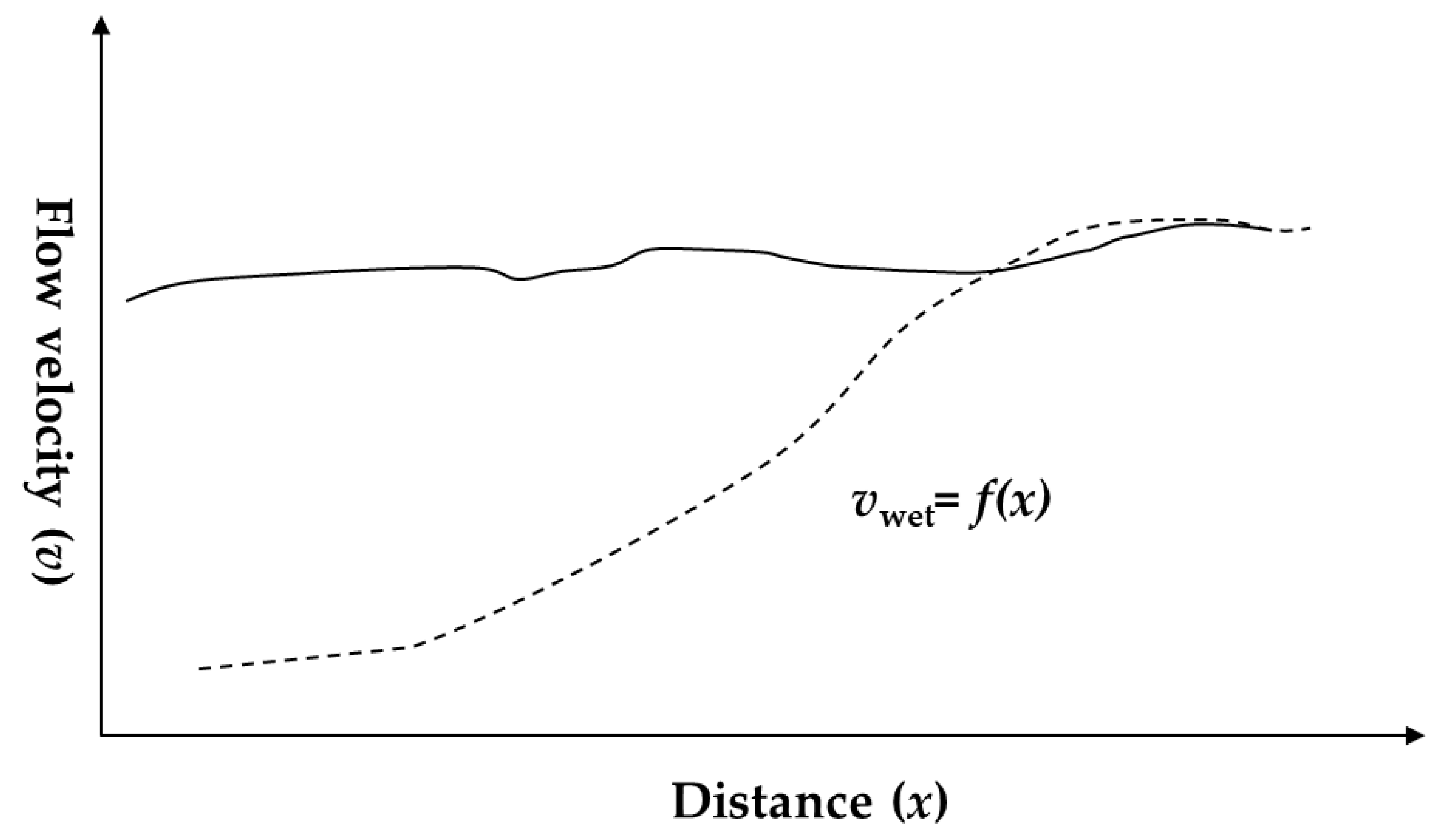
2.3.2. Defining the Upper Boundary

In the wet season, the rising lake water level has a blocking effect on the river water that is entering the lake, and lake water reinjection may occur [40]. The flow of a river that enters the lake will be blocked and the flow velocity will decrease in response. In the dry season or a season with normal water availability, the low water level of the lake has a weaker blocking effect on the river, so the flow velocity of the river changes less than at other times, with only small fluctuation around a mean flow velocity [33], as shown in Figure 3.
Based on the interaction between river and lake water during the wet and dry seasons, which we simulated using the coupled 1D and 2D hydrodynamic models, we extracted the flow velocity of the river at positions ranging from the lake’s inlet to the upstream boundary during the wet and dry seasons, and used this data to establish the corresponding relationship between the flow velocity and the distance along the river measured from the position of the lake’s inlet (Figure 4). During the dry season or a season with normal water availability, the flow velocity of the river changes little, showing a small fluctuation around a mean flow velocity, and it is relatively close to a constant. During the wet season, fluctuation around the mean is greater. We fit a functional equation to this data for the relationship between the flow velocity and the distance from the lake’s inlet Equation (1):
vwet = f(x)
where vwet denotes the flow velocity at each point along the river during the wet season, and x represents the distance of that point along the river to the lake’s inlet.
To solve for f ( x ) , the second derivative of the functional equation that describes the relationship between the flow velocity and the distance of each point along the river from the inlet during the wet season, let the 2nd derivative f ( x ) = 0   and   the   3 rd   derivative   f ( x ) ( 3 ) 0 . By solving the functional equation, we can identify the inflection point where the functional equation changes from concave to convex. We then used the position of the inflection point, which is equal to its distance from the lake’s inlet. By verifying the coordinates of the inflection point against the functional relationship between the flow velocity and the distance along the river, we identified the position of the flow velocity mutation point, where the flow velocity changes from gradually increasing to stable fluctuation around a mean during the wet season, and used this to represent the upper boundary of the transition zone.

2.3.3. Defining the Lower Boundary

At the lower boundary of the zone where river water enters the lake, there is a velocity gradient in which the flow velocity decreases until the water reaches the same velocity as the lake water. We used the coupled 1D and 2D hydrodynamic models for the transition zone to simulate the distribution of flow velocities at the lower boundary. Based on the distribution of flow velocities, we calculated the flow velocity gradient between the three outermost velocity lines, where a gradient exists between three velocity lines: an upstream line (k), a downstream line (j) that represents the last line with a velocity greater than that of the lake water, and a line (i) intermediate between these two lines. The gradient is defined as follows,
G i j = V i V j l i j
where Gij represents the flow velocity gradient between velocity line i and velocity line j within the transition zone; vi and vj (m/s) represent the velocity of velocity lines i and j of the transition zone, respectively; and lij (km) is the physical distance between the two velocity lines. Gki is defined similarly.
Based on the calculation results, we compared the flow velocity gradients at the lower boundary, and selected the two velocity lines with the smallest flow velocity gradient or with a flow velocity gradient approaching 0; these lines represent the points where the flow velocity is as close as possible to the lake’s flow velocity. We defined the outermost of these lines as the lower boundary of the transition zone (Figure 5).

3. Case Study

3.1. Study Area

China’s Baiyangdian Lake, which lies between 115°38′ E and 116°07′ E and between 38°43′ N and 39°02′ N, covers a total area of 366.4 km2 (Figure 6). It is the largest freshwater lake in the North China Plain. Known as the “Pearl of North China”, Baiyangdian Lake takes in water from nine rivers within the Daqing River system, including the Zhulong River, Xiaoyi River, Tang River, Fu River, Bao River, Ping River, Cao River, and Xiaobai River, as well as the Baigou Canal. Among these many rivers, the Fu River and Baigou Canal have the most stable amount of water flowing into the lake. Located to the west of Baiyangdian Lake, the Fu River, with a total length of 62 km, has an average annual flow of about 1.44 m3/s. Located to the northeast of Baiyangdian Lake, the Baigou Canal is an artificial river that is 12 km long, and has an average annual flow of about 15.6 m3/s.

3.2. Hydrological Boundaries

We established a 1D hydrodynamic model of the Fu River and Baigou Canal using the MIKE11 module in the MIKE ZERO software platform (https://www.mikepoweredbydhi.com/products/mike-11). We calibrated the model and verified its outputs using data from 1 September 2017 to 28 February 2018 measured by hydrological stations at Wangting (115°39′49.38″ E, 38°49′45.87″ N) and Xingaifang (116°1′56.42″ E, 39°4′35.01″ N). For the 2D hydrodynamic model of Baiyangdian Lake, we used the model of Zhao et al. (2014) [41]. The 1D and 2D hydrodynamic models were coupled by using the MIKE FLOOD module; that is, the output flow velocities from the 1D model became the input flow velocities for the 2D model. The coupled model simulated the hydrodynamic processes in the transition zone from 1 March 2018 to 28 February 2019.
According to the simulation results produced by the coupled 1D and 2D hydrodynamic models of the transition zone, we have selected the measured and simulated water level data in Duancun hydrological station (115°57′5.20″ E, 38°50′40.33″ N) of Baiyangdian Lake, from 1 March to 1 September 2018, to evaluate the accuracy of the model. The coefficient of determination (R2) [42] is 0.912; and the Nash Sutcliffe efficiency coefficient (ENS) [43] is 0.933. The models we developed can accurately reflect the hydrodynamic changes in the study area and meet the accuracy requirements of defining the hydrological boundary in the transition zone of Baiyangdian Lake.

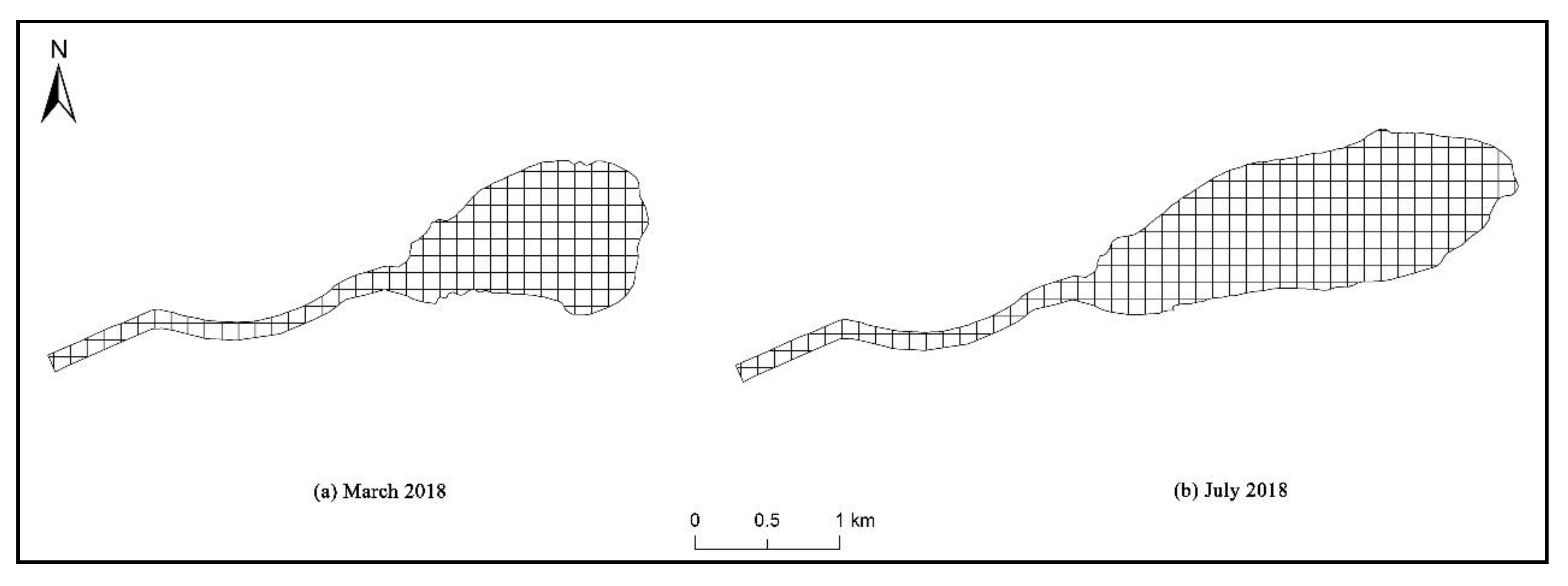
3.2.1. The Upper Boundary

We analyzed the simulation results produced by the coupled 1D and 2D hydrodynamic models of the river–lake transition zone. Using 100 m intervals, we extracted the velocity data for each interval from a distance of 0 km (at the lake’s inlet) to 3 km upstream from the lake’s inlet during the dry season and wet the season, Fu river is in March and July, Baigou Canal is in April and August. We used this data to establish the relationship between the flow velocity and the distance from the lake’s inlet along the river, to fit the functional equation that describes the relationship between the flow velocity and distance, to determine the location of the flow velocity mutation point during the wet season, and determine the upper boundary of the transition zone.
We extracted the flow velocity in each section of the Fu River in the transition zone with Baiyangdian Lake during the wet and dry seasons. Figure 7 shows the distribution of flow velocities along the river. Based on the velocity data during the wet season, we fitted a discrete equation for the distribution of flow velocities along the river. By taking the derivative of the fitting curve, we calculated the location of the function’s inflection point. These calculations are described in detail in Appendix A.1.1. In summary, the calculated results were x = 0.62 and x = 2.35 for the inflection points. From Figure 8, when x = 0.62, the flow velocity is constantly increasing rather than suddenly changing. When x = 2.35, there is a mutation in flow velocity where the flow velocity changes from gradually increasing to relatively stable fluctuation around a mean value. On this basis, we concluded that the upper boundary of the Fu River–Baiyangdian Lake transition zone occurs at 2.35 km upstream from the lake inlet.
We extracted the flow velocity in each section of the Baigou Canal for the transition zone with Baiyangdian Lake during the wet and dry seasons (Figure 9). Based on the velocity data during the wet season, we fitted the discrete equation for the distribution of flow velocities along the canal. By taking the derivative of the discrete equation, we plotted a fitting curve (Figure 10). By taking the derivative of the fitting curve, we calculated the inflection point of the function. Details of the calculation process are shown in Appendix A.1.2. In summary, the calculated values were x = 0.195 and x = 2.18 for the inflection points. From Figure 10, when x = 0.195, the flow velocity is constantly increasing rather than suddenly changing. When x = 2.18, there is a mutation in flow velocity such that the flow velocity changes from gradually increasing to stable fluctuation around a mean. We therefore concluded that the upper boundary of the Baigou Canal–Baiyangdian Lake transition zone is at 2.18 km upstream from the lake’s inlet.

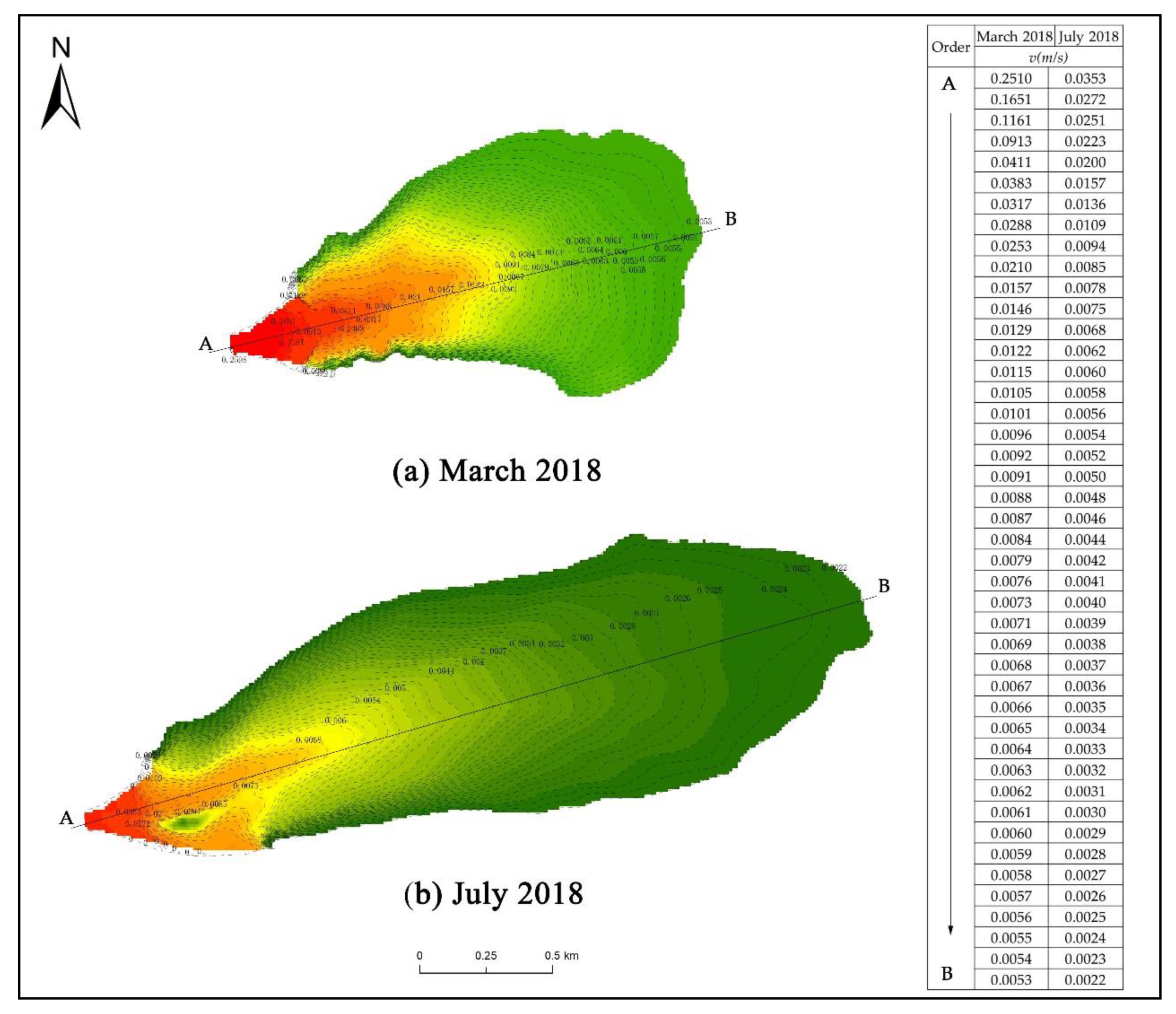
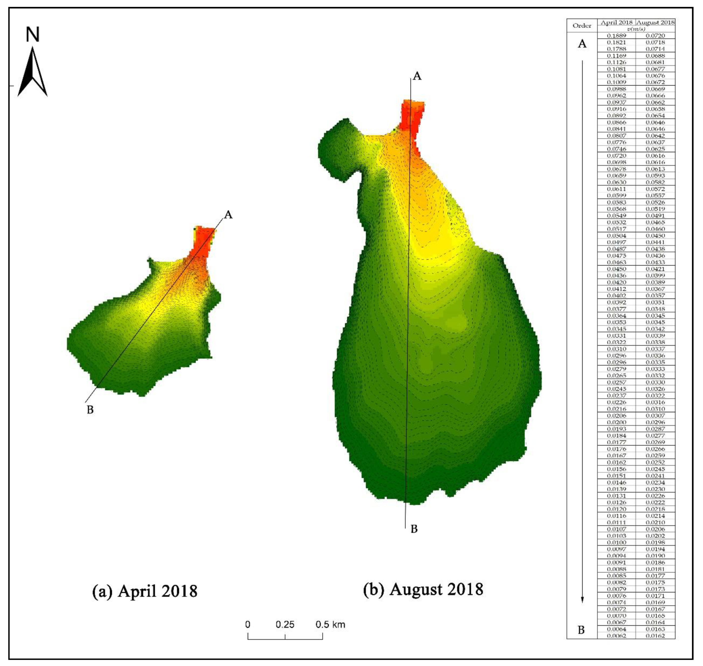
3.2.2. The Lower Boundary

Based on the results simulated by the coupled 1D and 2D hydrodynamic models, we extracted the monthly distribution of downstream flow velocities for the Fu River–Baiyangdian Lake and the Baigou Canal–Baiyangdian Lake transition zones from March 2018 to February 2019. We used this data to plot charts of the flow velocity. We calculated Gij and Gki, which represent the flow velocity gradients between the outermost flow velocity contour lines k, i, and j. These results let us compare the flow velocity gradients and select the two velocity lines with the smallest flow velocity gradient or a flow velocity gradient approaching 0. We used the line with the lowest velocity among the two velocity gradients as the lower boundary of the transition zone.
We extracted the distribution of flow velocities at the downstream end of the transition zone between the Fu River and Baiyangdian Lake from March 2018 to February 2019 and used the data to draw charts showing changes in the monthly distribution of flow velocity (Figure 11 and Appendix B Figure A1). Table 2 presents the numerical values of the flow velocity gradients between the outermost velocity lines.
Table 2 shows that the outermost flow velocity in the Fu River–Baiyangdian Lake transition zone ranged from 0.0020 to 0.0189 m/s, with the flow velocity gradient ranging from 0.02% to 0.22%. By comparing Gij and Gki, we can see that, during the simulation period from March 2018 to February 2019, the lower boundary was the second outermost velocity line i in July 2018, when Gij > Gki. In the remaining 11 months, when Gij < Gki, the flow velocity contour line j (the outermost velocity line) was the lower boundary.
We extracted the flow velocities for the Baigou Canal in the transition zone downstream from Baiyangdian Lake from March 2018 to February 2019 and used the data to draw charts showing the monthly distribution of flow velocity (Figure 12 and Appendix B Figure A2). We then calculated the flow velocity gradient between the outermost velocity lines (Table 3).
Table 3 shows that the outermost flow velocity of the Baigou Canal–Baiyangdian Lake Transition Zone ranged from 0.0032 to 0.0162 m/s, with the flow velocity gradient varying from 0.11% to 0.88%. By comparing Gij and Gki, we can see that during the simulation period from March 2018 to February 2019, the lower boundary was the flow velocity contour line i in October 2018, when Gij > Gki; that is, it was the second outermost velocity line. In the remaining 11 months, when Gij < Gki, the flow velocity contour line j (the outermost velocity line) represented the lower boundary.

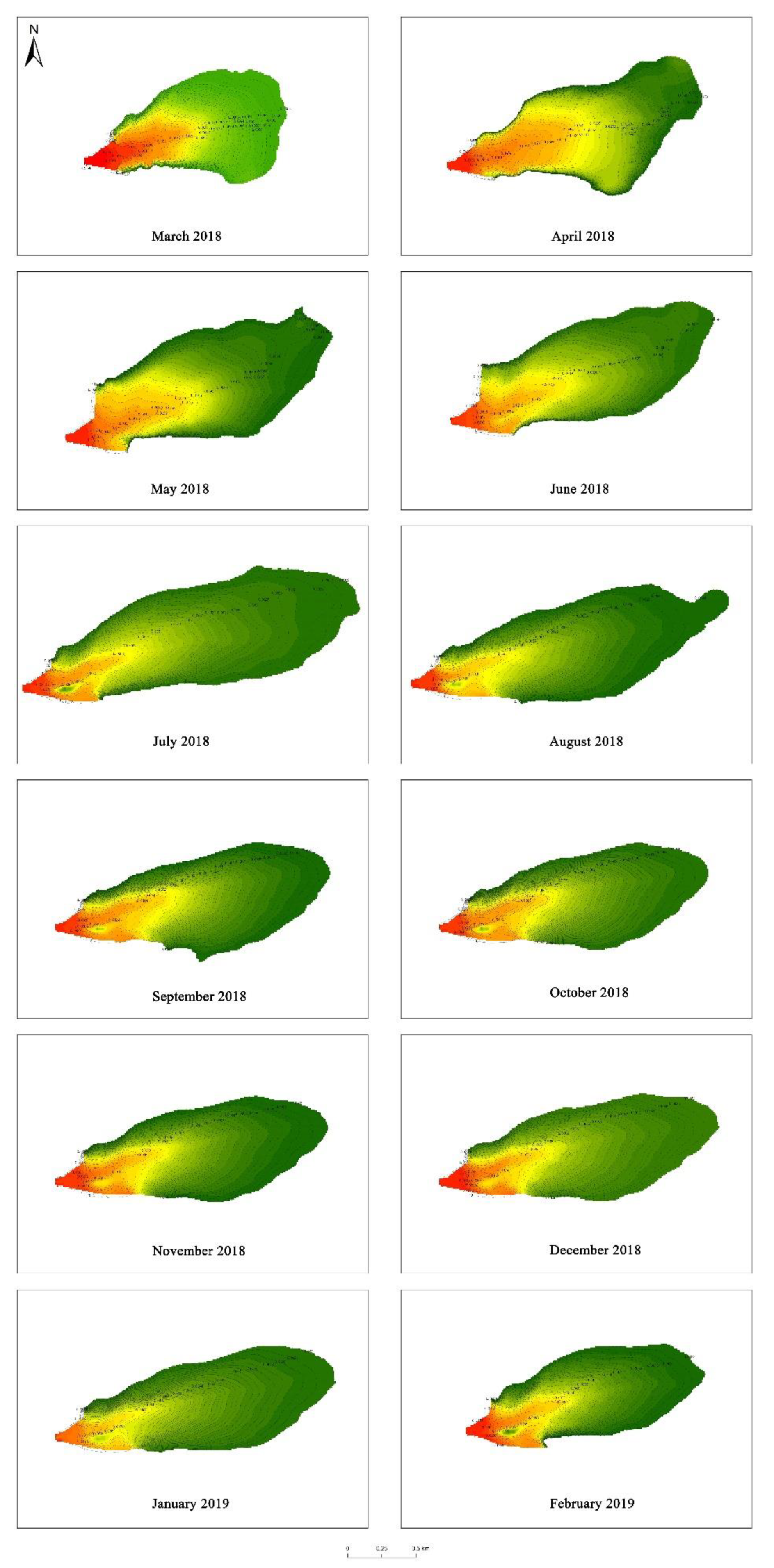
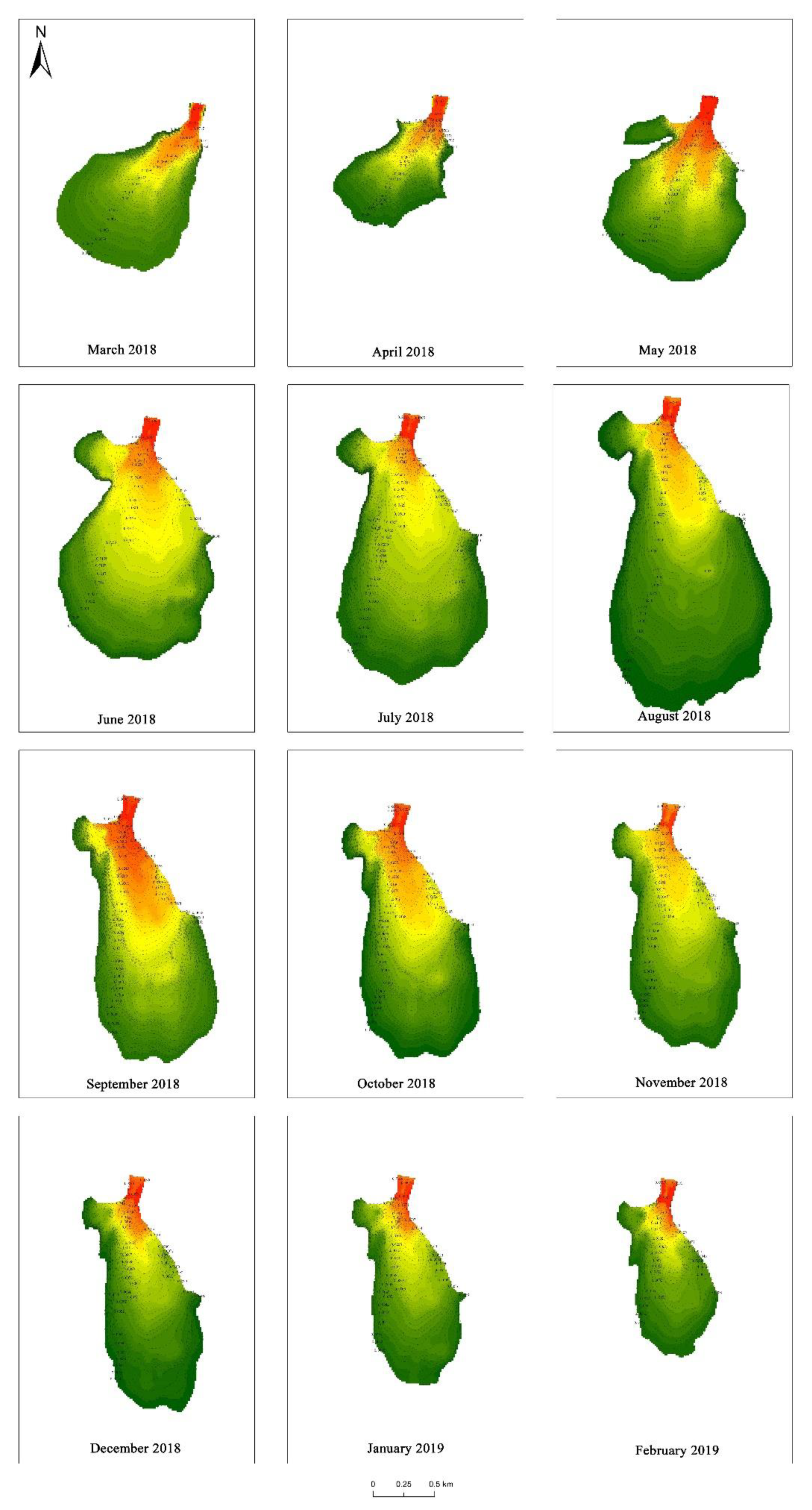
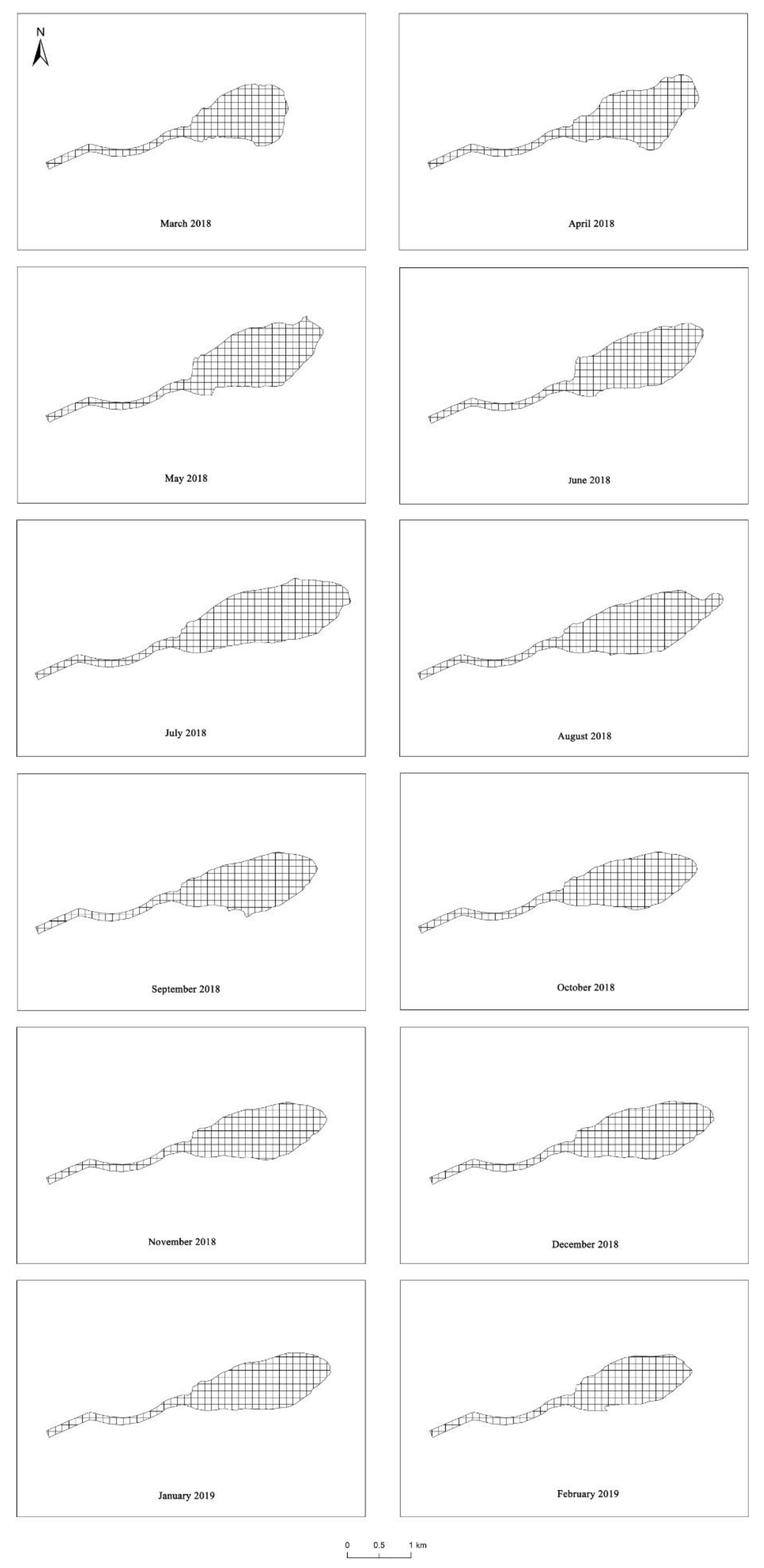
3.2.3. Dynamic Patterns of the Hydrological Boundary

The upper boundary of the transition zone was affected by the wet and dry seasons, but its position was relatively fixed within a given hydrological year. However, differences in the monthly discharge caused the position of the lower boundary to change dynamically. We calculated the area of the transition zone based on the water–land boundary and the hydrological boundary. Using remote sensing images of Baiyangdian Lake from 15 October 2018 with 15 m resolution, we performed manual interpretation to identify the land–water boundary, and imported the resulting images into version 10.5 of the ArcGIS software (www.esri.com). Based on these boundaries and the boundaries we calculated for the transition zone, we found the area of the transition zone in ArcGIS. These values reflect the dynamic changes of the hydrological boundary for the two transition zones that we studied (Figure 13 and Figure 14).
Figure 13 and Figure 14 and Table 4 show that from March 2018 to February 2019, the areas of the two transition zones generally increased, and then decreased in subsequent months. In July, the lower boundary of the Fu River–Baiyangdian Lake transition zone was farthest from the lake’s inlet, and the maximum area of the transition zone reached 2.603 km2. In March, the lower boundary was closest to the lake’s inlet, and the minimum area of the transition zone reached 1.598 km2. For the Baigou Canal–Baiyangdian Lake transition zone, its lower boundary was the farthest from the lake’s inlet in August, and the maximum area of the transition zone reached 2.762 km2. In April, the lower boundary was closest to the lake’s inlet, and the minimum area of the transition zone reached 0.901 km2.

4. Discussion

4.1. Objectivity of the Method

The interactions between river and lake water represent the main driving factor in the transition zone, and the strength of the interaction is directly reflected in the magnitude of the change in flow velocity [18]. The lake water level shows periodic changes between the wet and dry seasons [34]. During the wet season, the water level of the lake has a jacking effect on the river water that enters the lake, and this directly affects the river’s flow velocity [41]. In the dry season or a season with normal water availability, the river is basically in a state of natural flow, and the flow velocity will not be greatly affected [44,45]. After the river flows into the lake, a stagnant body of water appears at the front of the river water, and significantly blocks the river’s flow. As the water depth increases, the lake’s blocking effect increases, resulting in a rapid decrease in flow velocity [18]. In this paper, we developed a method of defining the hydrologic boundaries of the river–lake transition area to quantify these changes and express the scope of influence and intensity of the interaction between the river and lake water. Using this method, we analyzed the hydrologic boundaries, and confirmed the applicability of the method using a case study of the transition zones between the Fu River, Baigou Canal, and Baiyangdian Lake.
The method we developed improves on the previous method of defining the tail-reach of inflowing river water established by Wang et al. [33]. First, we used a hydrodynamic model of the transition zone to simulate the hydrodynamic conditions. Then, based on the simulation results, we extracted the flow velocity data, thereby eliminating the previous model’s dependence on the density of river hydrometric stations and the measured data, which makes the required data easier to obtain and improve the objectivity and feasibility of the method. Second, we improved the method for defining the lower boundary of the transition zone based on the distribution of flow velocity in this zone using the flow velocity gradient, which was not accounted for by the previous method. Finally, our method represents a complete definition of the hydrological boundaries, including both the upper and the lower boundaries of the transition zone.
The method based on water salinity gradients by Pritchard [29] and Li et al. [30] is more suitable for defining the boundary of the transition zone between rivers and oceans. The salt concentration gradient between a river and a lake is small and the difference is not obvious. Thus, a boundary definition method, based on a salt concentration gradient, can only determine an approximate range for the upper and lower boundaries, leading to ambiguous results. In contrast, our new method determines the specific location of the boundary according to quantitative criteria (i.e., based on the change of flow velocity), which is more objective and accurate. The boundary definition methods of Lei et al. [35] and Tian et al. [36], which are based on remote sensing analysis, requires a time series of remote sensing data to determine the boundary. Therefore, it requires a considerable amount of data and focuses on the inter-annual variation of the boundary. In contrast, our new method uses the data in a hydrological year to determine the boundaries of the transition zone. Therefore, it needs less data and focuses on the yearly variation of the boundaries of the transition zone. The two methods, are therefore, complementary. In addition, the accuracy of the model has a direct impact on the boundary and range of the transition zone. Generally, the higher the accuracy of the model, the more accurate the hydrological boundary is defined. Therefore, as an important pre-requirement for the determination of the transition zone boundaries, the developed hydrodynamic model should reach a certain accuracy to make the results credible and scientific. It is generally considered that when the R2 and ENS both exceed 0.7, it is considered as the goodness-of-fit of the model is better, and the model accuracy is higher [42]. The model we developed already meets this requirement. In future, more types of rivers and lakes should be combined to explore the model accuracy impact on the range of the transition zone further.
In fact, the transition zone is affected by many factors, including the hydrodynamics, hydrological conditions, topography, and aquatic environment [17]. It also shows longitudinal gradients of environmental factors, such as the current velocity, turbidity, nutrient load, and photosynthetic productivity [5]. Therefore, these factors should be considered during the process of defining the hydrological boundaries if the goal is to focus on more than just hydrology; for example, the boundaries for zones with different photosynthetic productivities may differ from the hydrological boundaries. Thus, additional methods can be developed and possibly integrated to develop a comprehensive method of defining the transition zone’s boundaries based on multiple factors or a single high-priority factor. These are all aspects of our study that need further research and improvement.

4.2. Universality of the Method

The method of defining the hydrological boundaries for the transition zone that we developed is only applicable to the transition zone where water from a river enters a lake. Based on the change of flow velocity caused by the interaction between the river and lake water, this method is suitable for a wide range of rivers and lakes with a relatively stable flow, distinct wet and dry seasons, and obvious interactions between the two bodies of water. This method is not suitable for seasonal rivers and lakes, rivers and lakes with a weak flow and indistinct dry and wet seasons, mountain rivers with large elevation differences, and rivers and lakes with water-blocking structures at the lake inlet. However, it should be possible to modify our model to account for these conditions.
In addition, our approach will need to be modified to account for transition zones with characteristics that differ from those in the present study, such as the transition zone where water leaves the lake and enters a river. In this type of transition zone, there are different interactions between the river and the lake. The relevant hydrodynamic processes, and changes in hydrological conditions, as well as the most appropriate method of defining the zone’s boundaries, will require further study.

5. Conclusions

Our method for defining the hydrological boundaries of a river–lake transition zone, which couples 1D and 2D hydrodynamic models to simulate the distribution of flow velocities, improves on previous descriptions of these zones. We established a functional relationship between the flow velocity and the distance along the river in both wet and dry seasons, and used this function to define the upper boundary using the flow velocity mutation point. We extracted the velocity flow field of the lake end of the transition zone and used the flow velocity gradient to define the lower boundary. We, then, demonstrated the approach using case studies of two Chinese river–lake transition zones.
Our two case studies clearly revealed the hydrological boundaries between the lake and a river or canal that enters the lake. The upper boundaries were relatively stable during the year, but the lower boundaries changed dynamically in response to discharge variations. For the Fu River–Baiyangdian Lake transition zone, the lower boundary was farthest from the lake’s inlet e in July and nearest to the lake’s inlet in March. For the Baigou Canal–Baiyangdian Lake transition zone, the lower boundary was farthest from the lake’s inlet in August and nearest to the lake’s inlet in April.
It will be important to improve our model in future research given the indispensable role the transition zone plays in material circulation and energy flows between rivers and lakes. It will be important to improve our definitions of the transition zone and its hydrological boundaries, as this will both, enrich the theoretical background on transition zones and provide a basis for subsequent studies of water quantity, water quality, and the aquatic ecological environment of transition zones.

Author Contributions

Conceptualization, K.T., W.Y. and Y.-w.Z.; data curation, X.-A.Y.; methodology, K.T., W.Y. and Y.-w.Z.; resources, K.T. and Y.-w.Z.; supervision, X.-A.Y., B.-s.C. and Z.-f.Y.; visualization, K.T.; writing—original draft, K.T. and Y.-w.Z.; writing—review and editing, W.Y. and Y.-w.Z. All authors have read and agreed to the published version of the manuscript.

Funding

This research was financially supported by the National key research and development program of China (grant 2017YFC0404505) and the Major Science and Technology Program for Water Pollution Control and Treatment (grant 2018ZX07110001).

Acknowledgments

We thank Geoffrey Hart for editing the English text of an early draft of this manuscript. We would like to extend special thanks to the editor and the anonymous reviewers for their valuable comments in greatly improving the quality of this paper.

Conflicts of Interest

The authors declare no conflict of interest. The funders had no role in the design of the study; in the collection, analyses, or interpretation of data; in the writing of the manuscript; or in the decision to publish the results.

Appendix A

Appendix A.1. Calculations for the Discrete Flow Velocity Functions

Appendix A.1.1. The Fu River–Baiyangdian Lake Transition Zone

The discrete equation for the distribution of flow velocities along the river was fitted as follows:
y = 0.0149 x 4 0.0087 x 3 + 0.1319 x 2 + 0.0711 x + 0.0332
where y represents the flow and x represents the distance from the lake inlet. The goodness of fit for the relationship (R2 = 0.95, p < 0.05) indicated a strong relationship between flow and distance. By taking the derivative of the discrete equation, we obtained the fitting curve shown in Figure 7. By taking the derivative of the fitting curve, we calculated the inflection point of the function:
y = 0.0596   x 3 0.0261 x 2 + 0.2638 x + 0.0711 y ( 2 ) = 0.1788   x 2 0.0522 x + 0.2638 y ( 3 ) = 0.3576 x 0.0522
If y(2) = 0 and y(3) ≠ 0, then x = 2.35 and x = 0.62 for the inflection points, corresponding to distances of 2.35 and 0.62 km, respectively.

Appendix A.1.2. The Baigou Canal–Baiyangdian Lake Transition Zone

Based on the flow velocity data during the wet season, we fitted the discrete equation for the distribution of flow velocities along the canal as follows:
y = 0.0093 x 4 0.0456 x 3 + 0.0245 x 2 + 0.1451 x + 0.0777
where y represents the flow and x represents the distance from the lake outlet. The goodness of fit for the relationship (R2 = 0.96, p < 0.05) indicated a strong relationship between flow and distance. By taking the derivative of the discrete equation, we obtained the fitting curve plotted in Figure 10. By taking the derivative of the fitting curve, we calculated the inflection point of the function:
y = 0.0372   x 3 0.1368 x 2 + 0.049 x + 0.1451 y ( 2 ) = 0.1116   x 2 0.2736 x + 0.049 y ( 3 ) = 0.2232 x 0.2736
If y(2) = 0 and y(3) ≠ 0, then x = 2.18 and x = 0.195 for the inflection points, corresponding to distances of 2.18, and 0.195 km, respectively.

Appendix B

Figure A1. Distribution of flow velocities of the Fu River–Baiyangdian Lake transition zone.
Water 12 00674 g0a1
Figure A2. Distribution of flow velocities of the Baigou Canal–Baiyangdian Lake transition zone.
Water 12 00674 g0a2
Figure A3. Areas of the Fu River–Baiyangdian Lake transition zone in each month. Numeric values are provided in Table 4.
Water 12 00674 g0a3
Figure A4. Areas of the Baigou Canal–Baiyangdian Lake transition zone in each month. Numeric values are provided in Table 4.
Water 12 00674 g0a4

References

  1. Holland, M.M. SCOPE MAB technical consultations on land scape boundaries: Report on A SCOPE MAB workshop on ecotones. Biol. Int. 1988, 17, 47–106. [Google Scholar]
  2. Birks, H.J.B. Aquatic ecotones—New insights from Arctic Canada. J. Phycol. 2014, 50, 607–609. [Google Scholar] [CrossRef] [PubMed]
  3. Kratz, T.K.; Frost, T.M. The ecological organisation of lake districts: General introduction. Freshw. Biol. 2000, 43, 297–299. [Google Scholar] [CrossRef]
  4. Willis, T.V.; Magnuson, J.J. Patterns in fish species composition across the interface between streams and lakes. Can. J. Fish Aquat. Sci. 2000, 57, 1042–1052. [Google Scholar] [CrossRef]
  5. Wetzel, R.G. Lake and river ecosystems. Limnology 2001, 37, 490–525. [Google Scholar]
  6. Jiang, X.; Zhang, L.; Gao, G.; Yao, X.; Zhao, Z.; Shen, Q. High rates of ammonium recycling in northwestern Lake Taihu and adjacent rivers: An important pathway of nutrient supply in a water column. Environ. Pollut. 2019, 252, 1325–1344. [Google Scholar] [CrossRef]
  7. Brandt, S.B.; Wadley, V.A. Thermal fronts as ecotones and zoogeographic barriers in marine and freshwater systems. Proc. Symp. Ecol. Soc. Aust. 1981, 11, 13–36. [Google Scholar]
  8. Forman, R.T.T.; Godron, M. Landscape Ecology; Wiley: New York, NY, USA, 1986. [Google Scholar]
  9. Naiman, R.J.; Décamps, H.; Pastor, J.; Johnston, C.A. The potential importance of boundaries of fluvial ecosystems. J. N. Am. Benthol. Soc. 1988, 7, 289–306. [Google Scholar] [CrossRef]
  10. Olden, J.D.; Jackson, D.A.; Peres-Neto, P.R. Spatial isolation and fish communities in drainage lakes. Oecologia 2001, 127, 572–585. [Google Scholar] [CrossRef]
  11. Daniels, R.A.; Morse, R.S.; Sutherland, J.W.; Bombard, R.T.; Boylen, C.W. Fish movement among lakes: Are lakes isolated. Northeast. Nat. 2008, 15, 577–589. [Google Scholar] [CrossRef]
  12. Zhang, R.; Gao, H.; Zhu, W.; Hu, W.; Ye, R. Calculation of permissible load capacity and establishment of total amount control in the Wujin River Catchment—A tributary of Taihu Lake, China. Environ. Sci. Pollut. Res. 2015, 22, 11493–11503. [Google Scholar] [CrossRef] [PubMed]
  13. Du, C.; Li, Y.; Wang, Q.; Liu, G.; Zheng, Z.; Mu, M.; Li, Y. Tempo-spatial dynamics of water quality and its response to river flow in estuary of Taihu Lake based on GOCI imagery. Environ. Sci. Pollut. Res. 2017, 24, 28079–28101. [Google Scholar] [CrossRef] [PubMed]
  14. Robinson, C.T.; Minshall, G.W. Longitudinal development of macroinvertebrate communities below oligotrophic lake outlets. Great Basin Nat. 1990, 50, 303–311. [Google Scholar]
  15. Welker, M.; Walz, N. Can mussels control the plankton in rivers?—A planktological approach applying a Lagrangian sampling strategy. Limnol. Oceanogr. 1998, 43, 753–762. [Google Scholar] [CrossRef]
  16. Jones, N.E.; Tonn, W.M.; Scrimgeour, G.J. Selective feeding of age-0 Arctic grayling in lake-outlet streams of the Northwest Territories, Canada. Environ. Biol. Fish. 2003, 67, 169–178. [Google Scholar] [CrossRef]
  17. Jones, N.E. Incorporating lakes within the river discontinuum: Longitudinal changes in ecological characteristics in stream–lake networks. Can. J. Fish. Aquat. Sci. 2010, 67, 1350–1362. [Google Scholar] [CrossRef] [Green Version]
  18. Qi, Y.L.; Liu, X.Y.; Yang, S.Y.; Zhang, T.; Li, C.S.; Xie, X.K. Hydrodynamic characteristics and geological significance of estuaries of inland lake delta. Lithol. Res. 2015, 27, 49–55. [Google Scholar]
  19. Ping, J. Jet Theory and Application; Astronautic Publishing House: Beijing, China, 1995; pp. 74–211. [Google Scholar]
  20. Leveau, M.; Lochet, F.; Goutx, M.; Blanc, F. Effects of a plume front on the distribution of inorganic and organic matter off the Rhone River. Hydrobiologia 1990, 207, 87–93. [Google Scholar] [CrossRef]
  21. Chen, S.; Huang, W.; Chen, W.; Wang, H. Remote sensing analysis of rainstorm effects on sediment concentrations in Apalachicola Bay, USA. Ecol. Inform. 2011, 6, 147–155. [Google Scholar] [CrossRef]
  22. Zhang, Y.; Shi, K.; Zhou, Y.; Liu, X.; Qin, B. Monitoring the river plume induced by heavy rainfall events in large, shallow, Lake Taihu using MODIS 250 m imagery. Remote Sens. Environ. 2016, 173, 109–121. [Google Scholar] [CrossRef]
  23. Timms, B.V. A study of the Werewilka Inlet of the saline Lake Wyara, Australia—A harbour of biodiversity for a sea of simplicity. Hydrobiologia 2001, 466, 245–254. [Google Scholar] [CrossRef]
  24. Moore, J.S.; Hendry, A.P. Both selection and gene flow are necessary to explain adaptive divergence: Evidence from clinal variation in stream stickleback. Evol. Ecol. Res. 2005, 7, 871–886. [Google Scholar]
  25. Sharpe, D.M.T.; Räsäsanen, K.; Berner, D.; Hendy, A.P. Genetic and environmental contributions to the morphology of lake and stream stickleback: Implications for gene flow and reproductive isolation. Evol. Ecol. Res. 2008, 10, 849–866. [Google Scholar]
  26. Statzner, B.; Higler, B. Stream hydraulics as a major determinant of benthic invertebrate zonation patterns. Freshw. Biol. 1986, 16, 127–139. [Google Scholar] [CrossRef]
  27. Foster, G.N. Conserving insects of aquatic and wetland habitats, with special reference to beetles. In The Conservation of Insects and Their Habitats; Collins, N.M., Thomas, J.A., Eds.; Academic Press: London, UK, 1991; pp. 237–262. [Google Scholar]
  28. Maitland, P.S. Biology of Fresh Waters; Springer: New York, NY, USA, 2013. [Google Scholar]
  29. Pritchard, D.W. Observations of circulation in coastal plain estuaries. Estuaries 1967, 13, 146–165. [Google Scholar]
  30. Li, C.C. On estuarine system and its automatic adjustment function–A case study: South China river. Acta Geogr. Sin. 1997, 64, 353–360. [Google Scholar]
  31. Muylaert, K.; Sabbe, K.; Vyverman, W. Changes in phytoplankton diversity and community composition along the salinity gradient of the Schelde estuary (Belgium/The Netherlands). Estuar. Coast. Shelf. Sci. 2009, 82, 335–340. [Google Scholar] [CrossRef]
  32. Li, C.C. Process and Evolution of Estuary in Southern China; Science Press: Beijing, China, 2004; pp. 1–20. [Google Scholar]
  33. Wang, X.; Wang, Y.; Xiao, W.; Wang, G.; Zhu, W. Research on method of defining tail-reach of inflowing river. Water Resour. Hydrol. Eng. 2013, 44, 44–47. [Google Scholar]
  34. Chen, J.; Li, B.; Deng, L.H.; Yu, M.T.; Yan, C.M. Advances in river pattern problems of tail reach for inflow rivers. Adv. Sci. Technol. Water Resour. 2019, 39, 79–85. [Google Scholar]
  35. Lei, S.; Zhang, Z.; Zhang, X.P. Analysis on tail channel evolution of 5 main rivers of Poyang lake based on remote sensing technology. Yangtze River 2014, 45, 27–31. [Google Scholar]
  36. Tian, J.; Zhang, Z. Study on the evolution of Xiuhe Weilv estuary based on remote sensing. J. East. Chin. Univ. Technol. (Nat. Sci.) 2016, 39, 94–99. [Google Scholar]
  37. Zhu, C.; Zhang, X.; Huang, Q. Four decades of estuarine wetland changes in the Yellow River delta based on Landsat observations between 1973 and 2013. Water 2018, 10, 933. [Google Scholar] [CrossRef] [Green Version]
  38. Yan, B.; Jia, Y.; Hinwood, J.B. Use of one-dimensional modelling in estuary management: Entrance depth—model calibration. J. Coast. Conserv. 2013, 17, 191–196. [Google Scholar] [CrossRef]
  39. Ai, X.; Jiang, J.; Liang, Q.; Huang, Q. Large-scale hydrodynamic modeling of the middle Yangtze River Basin with complex river–lake interactions. J. Hydrol. 2013, 492, 228–243. [Google Scholar]
  40. Munier SLitrico, X.; Belaud, G.; Malaterre, P.O. Distributed approximation of open-channel flow routing accounting for backwater effects. Adv. Water Resour. 2008, 31, 1590–1602. [Google Scholar] [CrossRef] [Green Version]
  41. Zhao, Y.W.; Xu, M.J.; Xu, F. Development of a zoning-based environmental–ecological coupled model for lakes: A case study of Baiyangdian Lake in northern China. Hydrol. Earth Syst. Sci. 2014, 18, 2113–2126. [Google Scholar] [CrossRef] [Green Version]
  42. Legates, D.R.; McCabe, J.G. Evaluating the use of “goodness-of-fit” measures in hydrologic and hydroclimatic model validation. Water Resour. Res. Sci. 1999, 35, 233–241. [Google Scholar] [CrossRef]
  43. Nash, J.E.; Sutcliffe, J.V. River flow forecasting through conceptual models: Part I-A discussion of principles. J. Hydrol. Sci. 1970, 10, 282–289. [Google Scholar] [CrossRef]
  44. Shao, X.J.; Wang, X.K. Introduction to River Dynamics; Tsinghua University Press: Beijing, China, 2005. [Google Scholar]
  45. Zhang, C.S.; Liu, B.Z. Physical simulation of formation process in distributary channels and debouch bars on delta. Earth Sci. Front. 2000, 7, 168–176. [Google Scholar]
Figure 1. Locations of the upper and lower boundaries in the river–lake transition zone.
Water 12 00674 g001
Figure 2. Process for defining the hydrological boundaries in the river–lake transition zone.
Water 12 00674 g002
Figure 3. Components of the upper boundary of the river–lake transition zone.
Water 12 00674 g003
Figure 4. Relationship between the flow velocity (v) and the distance along the river (x) measured from the lake’s inlet (see Figure 3 for the inlet’s location); the same function was used in the wet and dry seasons.
Water 12 00674 g004
Figure 5. Diagram of the flow velocity gradient at the lower boundary of the river–lake transition zone.
Water 12 00674 g005
Figure 6. Location of the study area, of Baiyangdian Lake, and of the main rivers that enter the lake.
Water 12 00674 g006
Figure 7. Flow velocities along Fu River during the dry (March) seasons and wet (July) as a function of distance from the lake’s inlet.
Water 12 00674 g007
Figure 8. Fitted curve of flow velocities along the river during wet season (July) as a function of distance from the lake inlet.
Water 12 00674 g008
Figure 9. Flow velocities along the Baigou Canal during the dry (April) seasons and wet (August) as a function of distance from the lake’s inlet.
Water 12 00674 g009
Figure 10. Fitted curve for flow velocities along the Baigou Canal during the wet season (August) as a function of distance from the lake’s inlet.
Water 12 00674 g010
Figure 11. Distribution of flow velocities in the Fu River–Baiyangdian Lake transition zone. (a) March 2018, when the range of the transition zone is smallest, (b) July 2018, when the range is largest. Charts for the flow fields in other months are shown in Appendix B Figure A1.
Water 12 00674 g011
Figure 12. Distribution of flow velocity in the Baigou Canal–Baiyangdian Lake transition zone. (a) April 2018, when the range of the transition zone was smallest, (b) August 2018, when the range was largest. Charts for the flow fields in other months are shown in Appendix B Figure A2.
Water 12 00674 g012
Figure 13. Area of the Fu River–Baiyangdian Lake transition zone. (a) March 2018, when the area was smallest, and (b) July 2018, when the area was largest. Charts for the area in other months are shown in Appendix B Figure A3. Numeric values of the areas are shown in Table 4.
Water 12 00674 g013
Figure 14. Area of the Baigou Canal–Baiyangdian Lake transition zone. (a) April 2018, when the area was smallest, and (b) August 2018, when the area was largest. Charts for the area in other months are shown in Appendix B Figure A4. Numeric values of the area are shown in Table 4.
Water 12 00674 g014
Table 1. Definitions of the river–lake transition zone.
NameDefinitionSource/References
Zone of transitionThe zone is from a lotic to a lentic environment or vice versa. This zone of transition may also be described as an ecotone.Naiman et al., 1988/[9]
Transition from stream to lakeThe transition from stream to lake is the zone where the water changes from a relatively shallow, fast-flowing habitat to a relatively deep, slow-flowing habitat.Willis and Magnuson, 2000/[4]
River–lake transition zoneThe transition zone occurs between a stream and a lake, and constitutes an ecotone.Kratz and Frost, 2000/[3]
Littoral zone of a lakeThe littoral zone represents a transition between a riverine zone and a lake zone, and exhibits a longitudinal gradient of environmental factors such as current velocity, turbidity, and photosynthetic productivity.Wetzel, 2001/[5]
Lake inlet and outletLake inlet and outlet streams are transition zones that provide migratory pathways for organisms within a stream–lake network.Olden et al., 2001/[10]; Jones et al., 2003/[16]; Daniels et al., 2008/[11]
Stream–lake networksThe staggered waters that form when rivers connect to lakes.Jones, 2010/[17]
River–lake transitional zonesRiver–lake transitional zones are “the hotspots” of nutrient cycling processes and have a profound impact on the lake’s ecological environment.Du et al., 2017/[13]
Table 2. Calculation of the flow velocity gradients Gij and Gki in the Fu River–Baiyangdian Lake transition zone. Figure 5 shows the positions of lines k, i, and j.
TimeFlow Velocity Contour Line (m/s)Distance (km)Flow Velocity Gradient (%)Lower Boundary
kijlkilijGkiGij
March 20180.00550.00540.00530.0790.0810.130.12Velocity line j
April 20180.01910.01900.01890.0450.0620.220.16Velocity line j
May 20180.00610.00600.00590.0800.0890.130.11Velocity line j
June 20180.00600.00590.00580.0630.2160.160.05Velocity line j
July 20180.00240.00230.00220.3520.1400.030.07Velocity line i
August 20180.00260.00250.00240.1040.4760.100.02Velocity line j
September 20180.00330.00320.00310.0730.0960.14 0.10 Velocity line j
October 20180.00280.00270.00260.0830.1150.12 0.09 Velocity line j
November 20180.00280.00270.00260.1220.1470.08 0.07 Velocity line j
December 20180.00360.00350.00340.1000.1340.10 0.07 Velocity line j
January 20190.00220.00210.00200.1240.1580.08 0.06 Velocity line j
February 20190.00300.00290.00280.0920.1350.11 0.07 Velocity line j
Table 3. Calculation of the flow velocity gradients Gij and Gki in the Baigou Canal–Baiyangdian Lake transition zone. Figure 5 shows the positions of lines k, i, and j.
TimeFlow Velocity Contour Line (m/s)Distance (km)Flow Velocity Gradient (%)Lower Boundary
kijlkilijGkiGij
March 20180.00510.00480.00450.0510.0670.59 0.45 Velocity line j
April 20180.00670.00640.00620.0340.0270.88 0.74 Velocity line j
May 20180.00850.00810.00790.0530.0280.75 0.71 Velocity line j
June 20180.00950.00940.00930.0130.0150.77 0.67 Velocity line j
July 20180.01110.01090.01070.0220.0240.91 0.83 Velocity line j
August 20180.01640.01630.01620.0240.0450.42 0.22 Velocity line j
September 20180.00610.00600.00590.0230.0260.43 0.38 Velocity line j
October 20180.00550.00540.00530.0250.0240.40 0.42 Velocity line i
November 20180.00590.00570.00550.0350.0420.57 0.48 Velocity line j
December 20180.00360.00350.00340.0370.0410.27 0.24 Velocity line j
January 20190.00340.00330.00320.0710.0940.14 0.11 Velocity line j
February 20190.00380.00360.00340.0580.0820.34 0.24 Velocity line j
Table 4. Areas of the river–lake transition zones.
TimeArea (km2)
Fu River–Baiyangdian Lake Transition ZoneBaigou Canal–Baiyangdian Lake Transition Zone
March 20181.5981.361
April 20181.9180.901
May 20182.1721.543
June 20182.0422.128
July 20182.6032.255
August 20182.2022.762
September 20181.9611.902
October 20181.8741.780
November 20181.9091.668
December 20181.9781.473
January 20191.9571.246
February 20191.6291.012

