On the Influence of the Main Floor Layout of Buildings in Economic Flood Risk Assessment: Results from Central Spain


Department of Geodynamics, Stratigraphy and Paleontology, Complutense University of Madrid, E-28040 Madrid, Spain
*
Author to whom correspondence should be addressed.
Water 2020, 12(3), 670; https://doi.org/10.3390/w12030670
Submission received: 30 December 2019
/
Revised: 31 January 2020
/
Accepted: 26 February 2020
/
Published: 1 March 2020
(This article belongs to the Special Issue Flood Risk Assessments: Applications and Uncertainties)
Abstract
:Multiple studies have been carried out on the correct estimation of the damages (direct tangible losses) associated with floods. However, the complex analysis and the multitude of variables conditioning the damage estimation, as well as the uncertainty in their estimation, make it difficult, even today, to reach one single, complete solution to this problem. In no case has the influence that the topographic relationship between the main floor of a residential building and the surrounding land have in the estimation of flood economic damage been analysed. To carry out this analysis, up to a total of 28 magnitude–damage functions (with different characteristics and application scales) were selected on which the effect of over-elevation and under-elevation of the main floor of the houses was simulated (at intervals of 20 cm, between −0.6 and +1 m). According to each of the two trends, an overestimation or underestimation of flood damage was observed. This pattern was conditioned by the specific characteristics of each magnitude–damage function, meaning that the percentage of damage became asymptotic from a certain flow depth value. In a real scenario, the consideration of this variable (as opposed to its non-consideration) causes an average variation in the damage estimation around 30%. Based on these results, the analysed variable can be considered as (1) another main source of uncertainty in the correct estimation of flood damage, and (2) an essential variable to take into account in a flood damage analysis for the correct estimation of loss.
1. Introduction
Floods are probably the most frequently recurring natural process affecting society in terms of time and space, regardless of their geographical location, as shown by the data collected by the International Disasters Database for the period 1900–2018 [1]. This is the main reason why flood risk management has become an essential tool from both a social and an economic perspective, with the objective of reducing losses associated with both sets of factors (features that constitute tangible and intangible flood damage). Assessing direct tangible damages (those direct damages resulting from the physical contact of floodwater with property and its contents), the economic flood losses have been increasing throughout the past half-century. In the last decade (2008–2018), the economic losses associated with floods exceeded 35 billion dollars [1] and, within this period, the flood losses exceeded 19 billion dollars (USD) in 2012 alone [2,3,4].
In this flood risk survey, the extension of the study area conditioned the analytical approach, and, as proposed by de Moel et al. [5], each work scale (supra-national, national or macro-scale, regional or meso-scale, and local or micro-scale) required the use of different methods of analysis, with their results needing to satisfy different purposes. A state-of-the-art review of study-related approaches, analysis techniques, results, uncertainties and validation processes of the results associated with each of these four work scales is collected in Reference [5]. Regarding this last point, the validation and calibration of the results involved fundamental elements that will require further study in the future (regardless of the work scale in the analysis), since they condition the usefulness of these studies for end users [6].
Flood risk study methodology changes significantly depending on the study area, so the work scales associated with supra-national or national assess are either generally based on multi-criterion analysis techniques (e.g., References [7,8,9]) or on scaled models (such as those proposed by References [3,10]). These approaches change when studies have a regional character, a situation where the combination of hydraulic models predominates (mainly those that combine 1D and 2D analysis, coupled 1D/2D models; e.g., References [11,12]) together with magnitude–damage functions associated with different land uses and obtained from the aggregation of damage models (e.g., References [13,14]) developed on a micro-scale level.
Finally, regarding micro-scale studies (local scale), the analysis techniques are similar to those used in regional studies, with an increase in the detail and specificity of the magnitude–damage functions used (e.g., References [15,16]) and in the precision of the hydraulic models, which in many cases directly become 2D models [17]. For the magnitude–damage functions, the value of the flow depth is normally used in the description of the flood magnitude [18], but there are still other factors (speed, duration, presence of pollutants, sediment concentration, etc.) that also play an important role in flood damage [19]. However, as described by Soetano and Proverbs [20], the flow depth variable is considered to be the main factor in the estimation of direct damage to buildings due to flooding, conditioning the spatial extent of the flood in X, Y, and Z. In hydraulic models, the main difference with regard to analyses carried out at other scales is their precision. This precision depends on the topography used, and although Moel et al. [5] determined a range between 1 and 25 m for the pixel size of the DTMs (digital elevation models) used, that value is currently set in the 1–5 m range (e.g., Reference [21]).
Nevertheless, not only the spatial resolution of the DTMs used is important for correct damage estimation [22], but also the accuracy of their altitude. This aspect is directly related to proper hydraulic modelling and the definition of flood areas, which have been studied since the end of the last century (e.g., References [23,24,25]). The effect of topographic precision is evident mainly in low relief areas [26], where the delimitation of flood zones may cause significant differences. More recently, the incorporation of LiDAR (light detection and ranging) data for the generation of DTMs has led to the increase in their accuracy and spatial resolution, which is a clear indication of progress made in the improvement of hydraulic models associated with complex topographic configurations such as urban areas. A clear example is the increase in the capacity to include buildings as topographic elements within 2D hydraulic models, which significantly improves damage estimation in areas where the availability of this type of information is limited [27]. Even so, these LiDAR data requires post–processing aimed at the correct classification of the points (land, vegetation, buildings, etc.) and their filtering, in order to enhance the quality and precision of 3D–derived surfaces. In this sense, Bodoque et al. [28] showed the need to post–process LiDAR data for their subsequent application in the estimation of flood damage, and how the accuracy of these data is influenced by the different types of terrain. This estimated flood damage can vary significantly in urban areas depending on how the initial topographic information (LiDAR data) is used [29], so that the control and validation of LiDAR data in these areas/built–up areas with tall buildings seems indispensable. On the other hand, since flow depth is the main variable from which the damages are estimated, the variable method assigned to each of the exposed elements is another factor in the uncertainty of correct damage estimation in urban areas [30].
From the above, increasing interest has been shown in the resolution and precision of the DTMs used as the basis for hydrodynamic (2D) flow modelling in the analysis of flood damage. These hydrodynamic models will provide us with information (mainly) on flow depth or flow velocity on which the quantification of flooding magnitude can be based. This magnitude can be subsequently correlated with the damage function used to estimate direct economic losses due to floods. However, throughout this flow analysis, an important component for correct damage estimation seems to have been left out: the relationship between the height of the main floor of the buildings and the elevation of the adjacent land. It is usually assumed that the topographic elevation of the land around a given building (streets, sidewalks, patios, unbuilt lots) is the same as that of the main floor of the adjacent house, serving as a reference for the start of the magnitude (depth)–damage functions. In this sense, Garrote–Revilla et al. [31], in a preliminary study carried out in the centre of the Iberian Peninsula, based on the use of the magnitude–damage functions proposed by the USACE (United States Army Corps of Engineers) [32,33], suggested that the influence of this variable can significantly modify (variations greater than 20%) the damage estimation associated with flood events.
This work constituted the first detailed research on the influence of the real topographic relationship between the main building floor (height of the first floor that directly leads to the doorway) and the correct estimation of the direct tangible damage associated with floods. For this reason, its results can be used as a reference for the suitability or need to consider this variable in risk studies on a micro–scale level. Application to wide areas may be more difficult due to the presence of heterogeneous building stocks. From the last point of view, more micro–scale analysis may be useful for establishing regional or general trends. The need for or suitability of the use of the variable should based on the differences found in the estimation of damages, and the significance level of those differences depending on the damage models (magnitude–damage functions) considered. Although the uncertainty (which may also be exposure–related, caused by the lack of knowledge about building characteristics) in damage estimation in houses caused by floods has been widely discussed, the relationship between the variable considered in the present paper and its uncertainty has not yet been analysed. The other two variables that are used in damage estimation must not be neglected: the exposure (depending on the elements that are present at the location involved and on the spatial distribution of the flood spot) and the vulnerability (defined by the lack of resistance of exposed elements to the flooding), which were not taken into account as independent variables in this survey, as vulnerability models were taken from previously proposed models. The results obtained showed a scenario in which the variations in the estimation of economic damages in residential buildings reach percentages and magnitudes similar to those obtained in previous studies focusing on other variables. The topographic difference between the main floor of a house and the surrounding land should be considered in damage mitigation or flood management as a basic factor for the correct estimation of damages and, consequently, as another possible source of uncertainty.
2. Materials and Methods
As mentioned in the previous section, the vulnerability of exposed elements is usually assessed based on damage models according to magnitude–damage functions. The present study assembled different magnitude–damage functions from various countries, extracted from international scientific and technical literature, to assess the direct and tangible damages in residential buildings. In addition to different geographical areas, these functions covered a wide spectrum of characteristics. They took into account whether there were basements in buildings or not, considering or not each separate building and its content and damages either as a monetary value or as a percentage of damage of the set of buildings and their content.
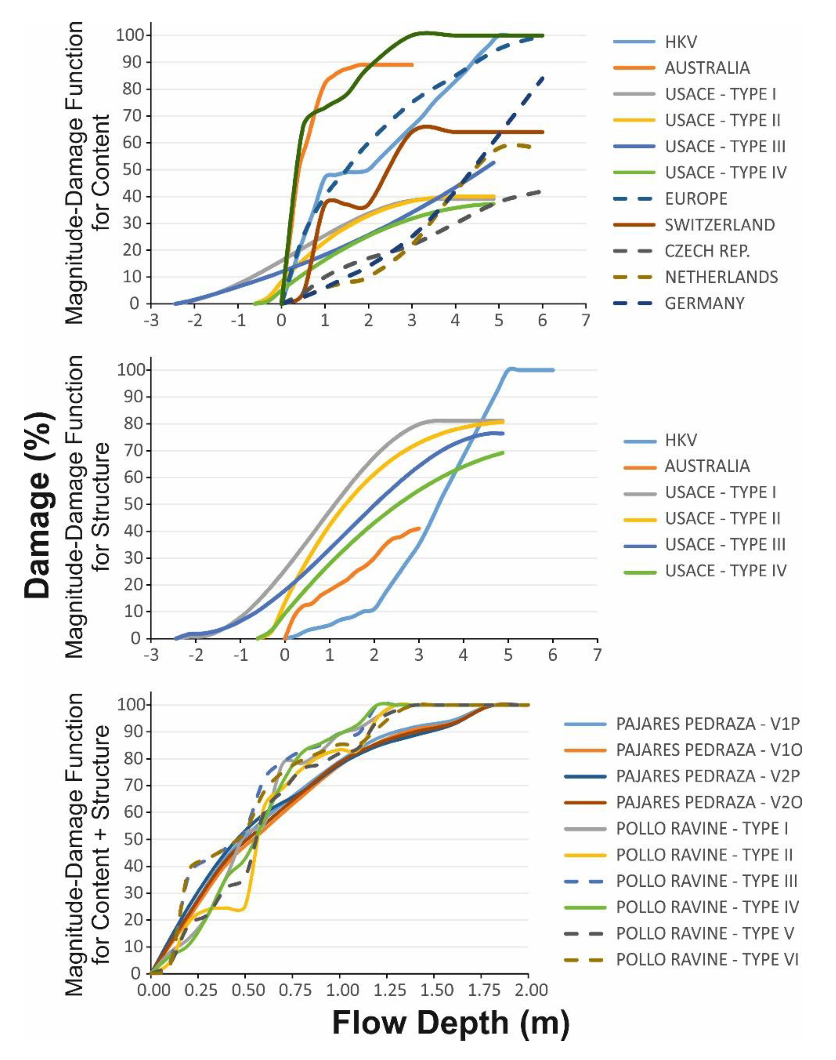
The ensemble of magnitude–damage functions used [21,32,33,34,35,36] and their characteristics (for USACE functions, Type I = one storey with basement, Type II = one storey without basement, Type III = two storeys with basement and Type IV = two storeys without basement) are shown in Table 1. There were 11 damage estimation models (proposed for different countries or regions), consisting of 28 magnitude–damage functions (Figure 1).
The estimation of the variable magnitude within magnitude–damage functions is generally carried out directly from intersection of the water depth data and the entities (generally polygons representing the boundaries of the housing) that indicate the exposed elements or through neighbour buffers of those polygons. This second option is widely used when the exposed elements (mainly buildings) are represented by cell height elevation (the most common method of representation; e.g., References [37,38]) up to the height of the roof of buildings in the digital surface model (DSM) used for hydraulic modelling. In these situations, water is forced to flow through the streets and cannot enter the buildings. Therefore, if no influence area of the building were used, the intersection between flow depth data and the exposed elements would not yield results. The flow depth value is generally defined by either the maximum value or the average value. The second option limits the possibilities of obtaining erroneous values linked to deficiencies in the topographic representation of the land in the DSM. However, as stated by Bermúdez and Zischg [30], the use of the maximum value makes the estimation of the flow depth more independent of the 3D mesh–building representation method of hydrodynamic models.
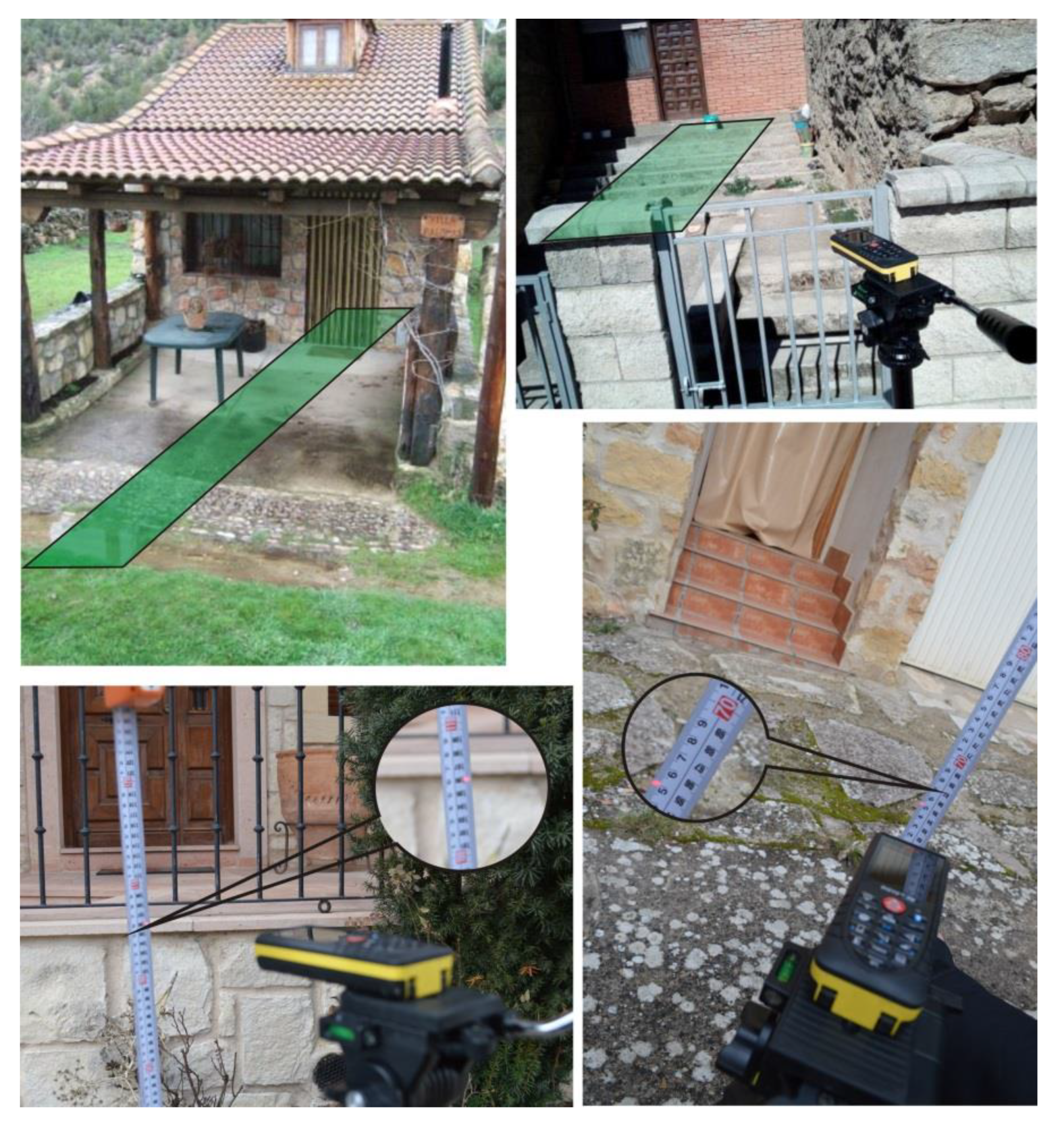
Therefore, the estimation of the water height (flood magnitude) will be made with respect to the flow depth value in the land surrounding the buildings. Thus, these situations do not consider the possibility of the building being over– or under–elevated compared to the surrounding land (Figure 2). For this reason, for each of the magnitude–damage functions used, different topographic scenarios were considered in which the effect of the possible over–and under–elevation of the buildings compared to the surrounding territory were analysed.
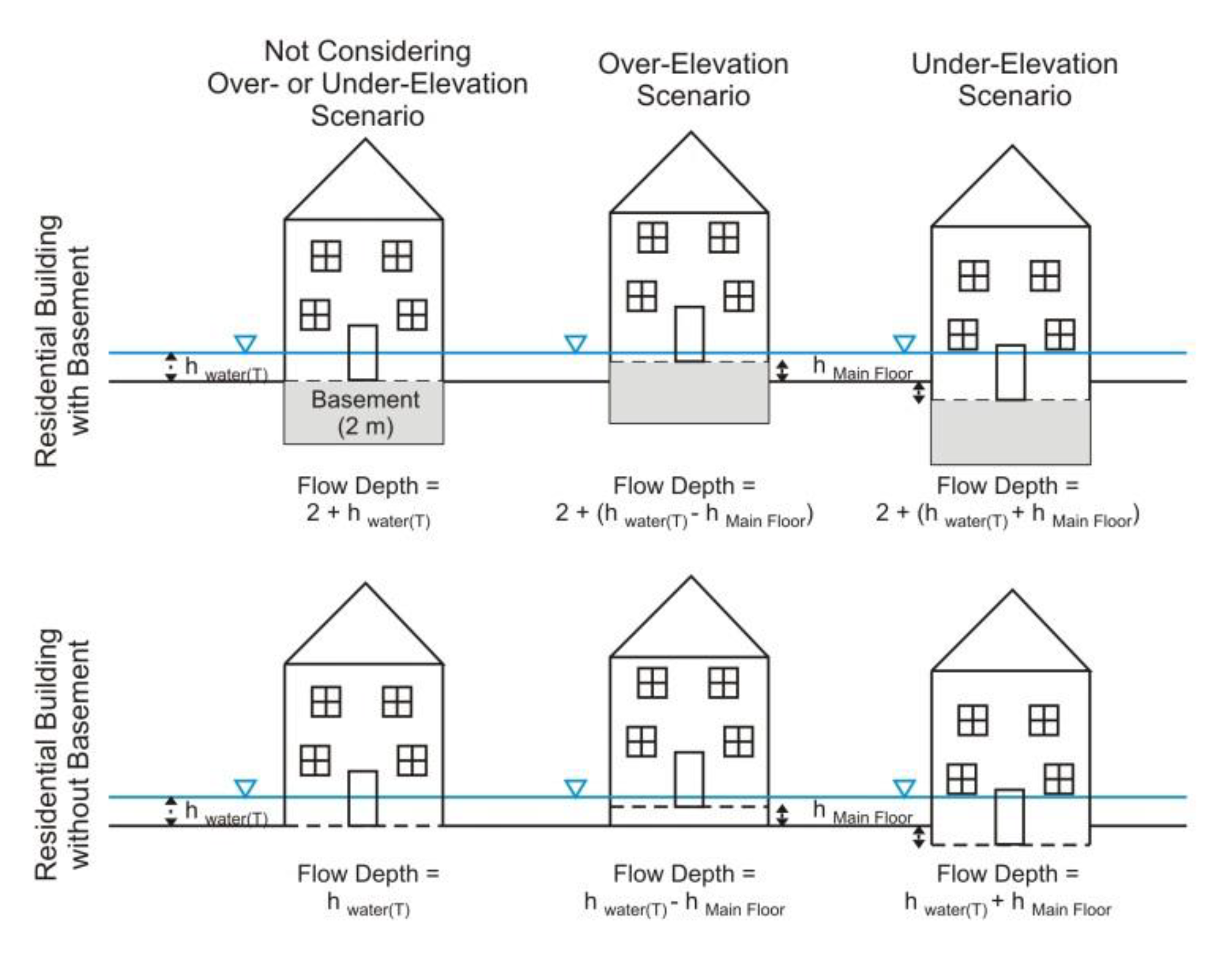
For each of these topographic scenarios, the variation in the damages with respect to the initial scenario was estimated, wherein no type of variation between the elevation of the main building floor and the surrounding land was taken into account (Figure 3). Depending on the characteristics of each magnitude–damage function used, the existence of basements was considered in the variations obtained in the damage estimation.
Hence, for every function analysed, successive scenarios were considered in which a topographic variation of 20 cm between the height of the main floor of the house and the adjacent land was incorporated. The range of variation between the level of the main floor and the surrounding land was varied between –60 cm and +100 cm, resulting in a series of nine analysis scenarios (including the initial one) of direct tangible damage due to flooding. The application of these over– and under–elevation thresholds to the main floor was based on the field work carried out by Garrote–Revilla et al. [31].
From the set of results obtained for each of the topographic scenarios considered, descriptive statistics and trend adjustment methods (mainly by estimating the changes in the damage to homes rates, and the graphic representation of these rates linked to the water depth) were applied to analyse the influence of the topographic relationship between the height of the main floor in the housing and the adjacent land. Thus, the influence of this variable was observed in the damage estimation, both in general (all the damage models used) and in a segregated manner in subsets defined according to the characteristics of the magnitude–damage functions used.
Finally, the results obtained in a real scenario are detailed in a later section, in which the estimation of the direct economic losses associated with floods in a small village in the centre of the Iberian Peninsula was carried out. In this specific case, residential dwellings were divided into the categories considered in each of the magnitude–damage functions proposed for use in this analysis. Subsequently, the average under– or over–elevation of the main floor in each of these categories was estimated with respect to the surrounding roads (streets). Lastly, the variation in the EAD value (expected annual damage) was determined based on the consideration or not of the variable “topographic relationship between main floor housing and roads” in the estimation of economic losses. In this last analysis (and due to the lack of real–time data) the economic valuation of the content and structure of residential buildings was considered as a constant value for each type of building.
3. Results
3.1. General Results for Magnitude–Damage Models
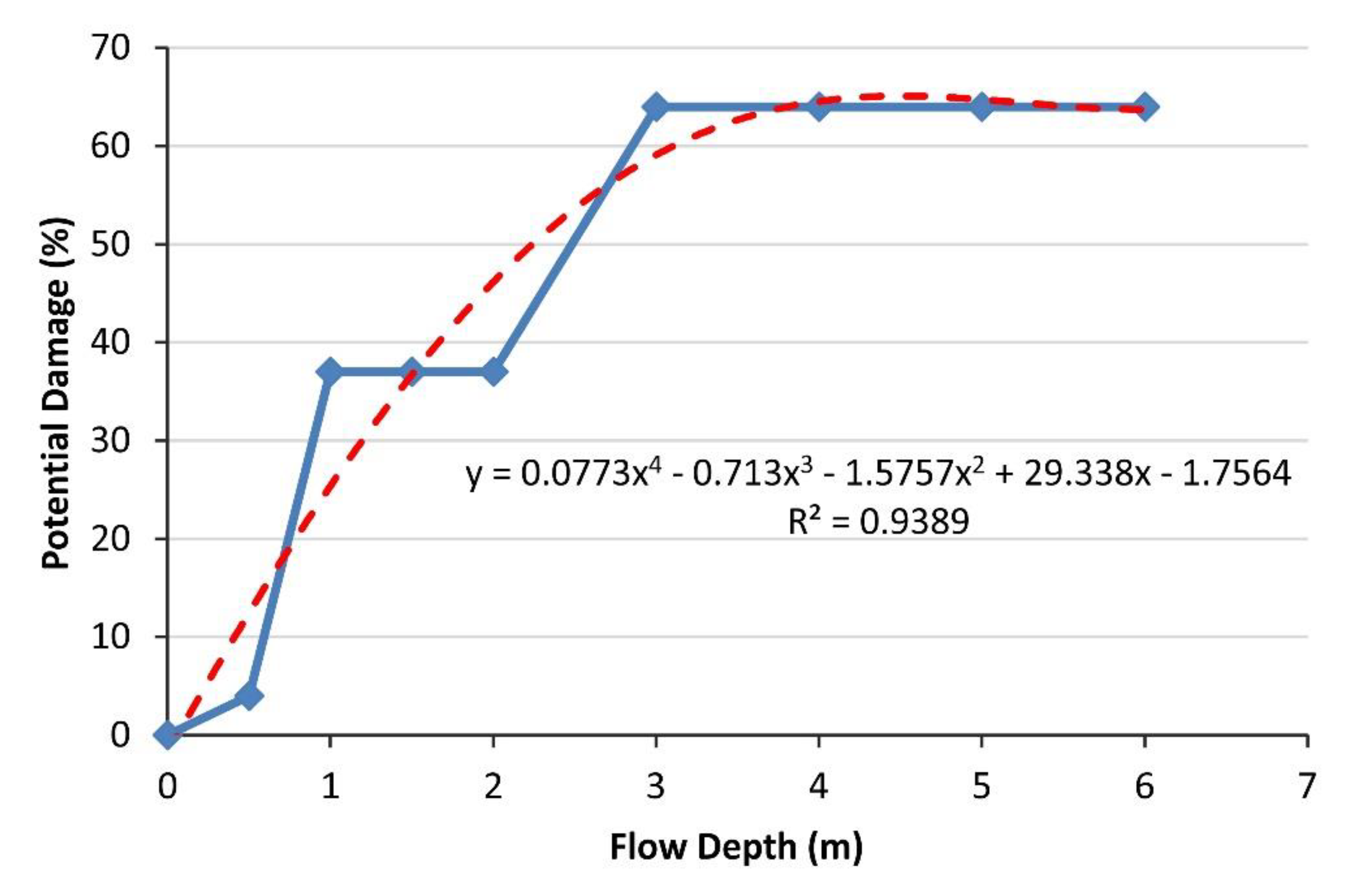
The damage models or magnitude–damage functions used were originally derived from a set of tables in which the percentage of damage associated with a series of flow depth values is related, instead of a mathematical formulation that determines a continuous function. For this reason, the first task required was to obtain a mathematical equation that defined the relationship between the “percentage of damage” variable with regard to the “flow depth” value. To attain this objective, the original data of a third– or fourth–degree polynomial function was adjusted, analysing the degree of adjustment of this polynomial function based on the R2 value. In general, R2 reached a value greater than 0.99. However, in the case of the magnitude–damage function used in Switzerland, a lower value was indicated (0.93). In this specific case, the magnitude–damage function showed a decrease in R2 due to the stepped form (Figure 4) presented by the original data.
The results obtained indicated how the flood damage estimation positively correlates with the topographic difference between the main floor of houses and the public roads or land surrounding these buildings. Thus, when buildings are over–elevated with regard to the adjacent land, there is a clear decrease in the percentage of estimated economic losses, and this effect is shown inversely in situations of under–elevation. In contrast, it can be seen that the sensitivity of the set of magnitude–damage functions or “damage models” used is varied (either between functions, or within the same function).
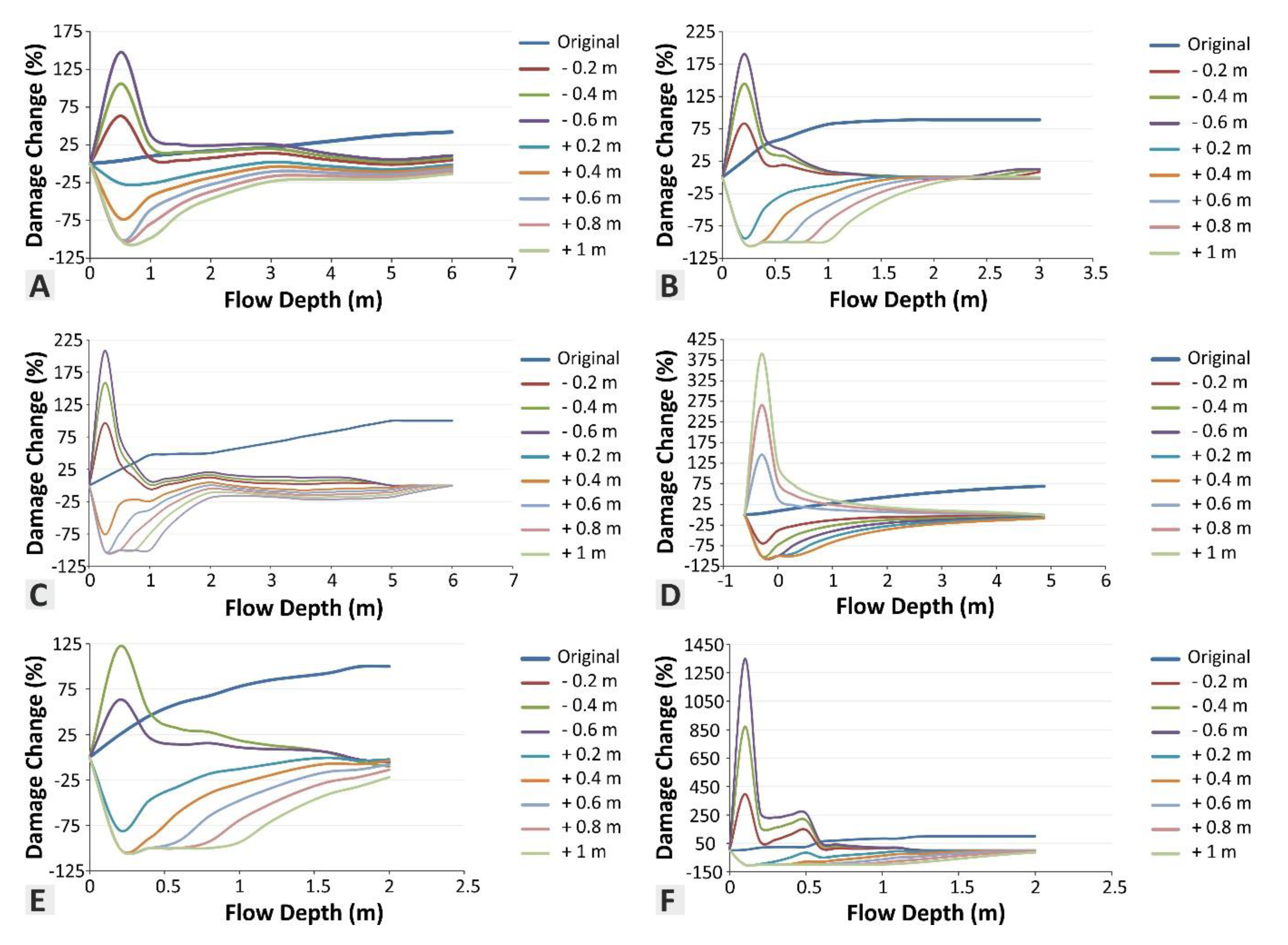
In general, the variation in the estimate of economic losses (damage rates) associated with flow depth values does not exceed a maximum of 100%. This situation occurs when the new topographic scenario considered eliminates the damages associated with a flow depth, so that the new percentage of damage is 0%. This pattern (Figure 5) was repeated in damage models with over a 1 m depth range (the maximum value considered for over–elevation in buildings with respect to the surrounding land), regardless of the damage model applied. It also considered either the “content” or the “structure”, or that these models have been proposed with a general scope (at the country level) or detail (at the locality or population level).
In the case of some specific functions such as Switzerland (Figure 4) or the Netherlands, both proposed in the JRC Report, or the equation of Australia (proposed by HKV Consultants) the regression lines did not reach 100% as the maximum value, as seen in Figure 4. This trend was due to the fact that these functions, which originated from statistical calculations, were not designed for extreme flood events such as those resulting from 4.5 m flow depth floods (Figure 4).
When the topographic effect analysed was the under–elevation of the house, the difference in the results (not considering or considering height difference between the main floor and surrounding land) was greater than in the over–elevation effect. This fact was not due to the trend of these results, since this always showed an increase in the percentage of economic damage, but in terms of the magnitude of these damage percentage variations. The increases in the percentage of damages (according to the results obtained) seemed greater in those magnitude–damage functions proposed for detailed analysis, than in the cases of those proposed for regional analysis, although it was not possible to affirm that the damage increase value ranges were totally independent. In scenarios in which an under–elevation of the building was simulated with respect to the surrounding land, there were more abrupt changes (than in over–elevation situations) in the variations in the percentage of economic damage, with a rapid rise and subsequent decrease in these variations.
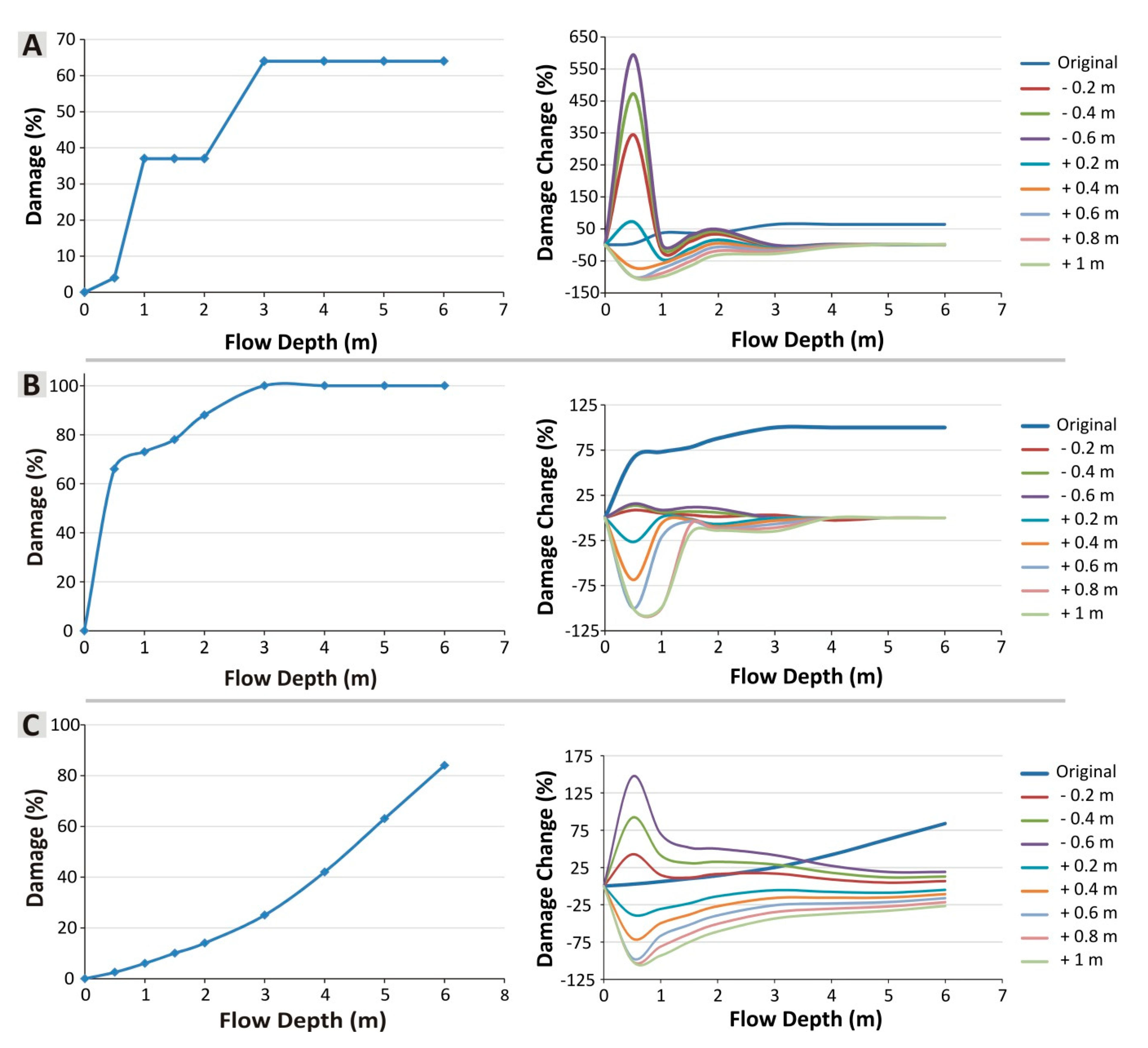
In any of the situations (over– or under–elevation), as we moved towards greater water depths there was a decrease in the differences of damage rates, so the effect of the main floor elevation from the surrounding land became negligible. When we moved towards the maximum flow depth values analysed in each magnitude–damage function, the damage percentage variations (associated with the different topographic scenarios proposed) were generally below 10%. This situation can be seen clearly in the damage change–flow depth graphs on the right of the Figure 6, related to magnitude–damage models of Switzerland (A), United Kingdom (B) and Germany (C). In the three examples, the damage change percentage increased with respect to the original damage values when the height of the main floor was under the street level. In contrast, when raising the elevation, the damage change percentage decreased, reaching negative values. Both trends stabilized when flow depth reached between 2 and 3 m, because at this point, the over– or under–elevation of the main floor level dis not influence the final damage.
The characteristics of the magnitude–damage function used had a clear influence on the damage percentage variation, both in the maximum flow depth considered (ranging from 2 m to more than 5 m), and in the maximum percentage of damage associated with these depths (which varied from percentages slightly higher than 40% to percentages of 100%). In the case of functions where the percentage of damage became asymptotic around a given flow depth value, the variations in that percentage associated with the topographic scenarios proposed were minor. An example of the above (Figure 6) would be the magnitude–damage functions related to countries such as the United Kingdom, Switzerland and the USA, or those proposed by Salazar Galán [35].
3.2. Local Results at Navaluenga (Central Spain)
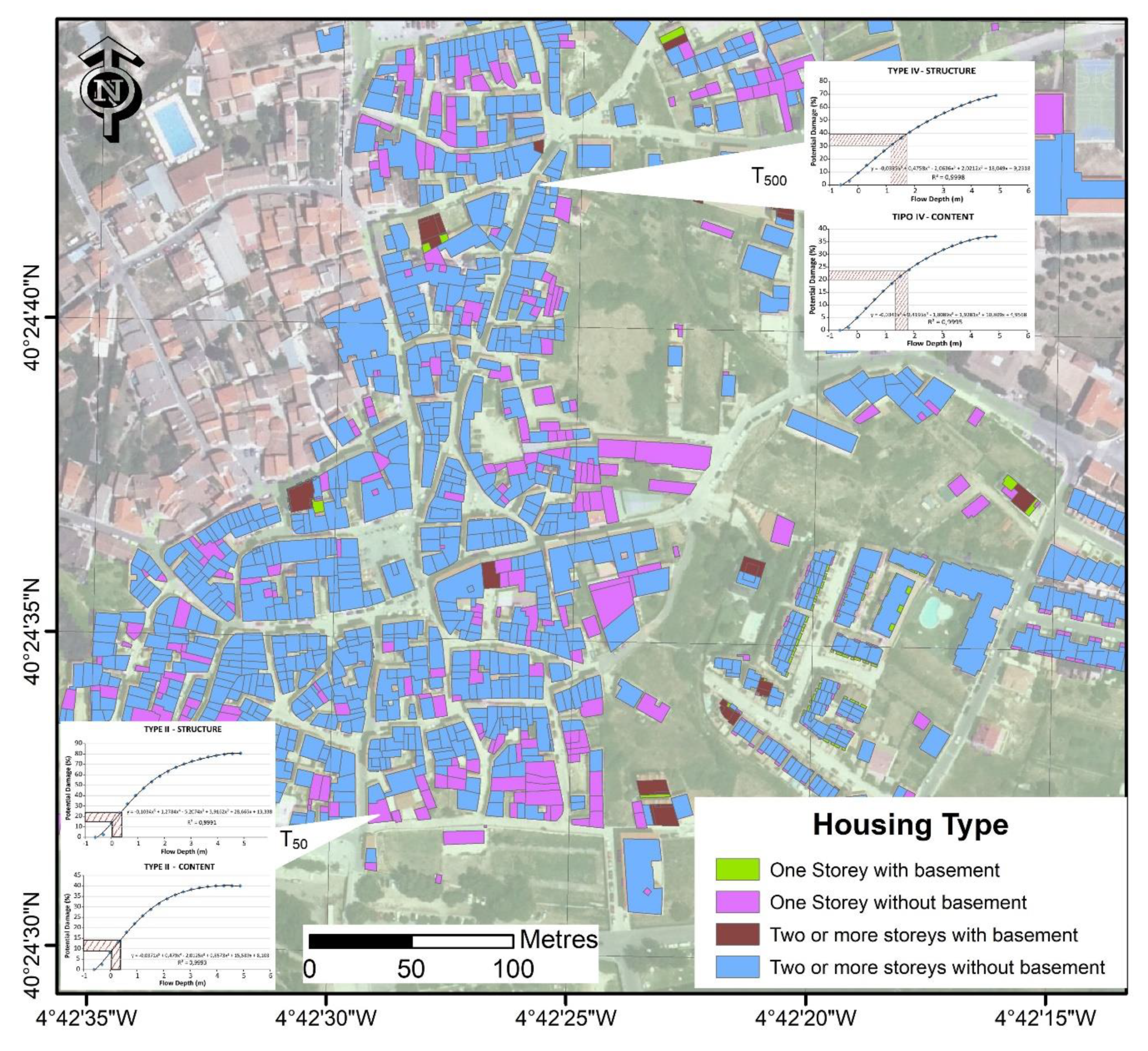
As a practical example of the analyses detailed above, the town of Navaluenga (Ávila, Central Spain) was used in order to determine the influence that the topographic relationship between buildings and surrounding lands had on the estimation of flood damages. The magnitude–damage functions applied were those proposed by the USACE and the buildings were classified into four groups. Depending on the number of dwellings included in each group, the topographic relationship (Z axis) between the main floor of the building and the surrounding land was estimated either for the total class of buildings or for a subset (statistically representative) of the buildings of the corresponding class.
In the studied town, the total number of dwellings amounts to 2256, which are distributed as follows (depending on the categories covered by USACE): 109 Type I housing, 621 Type II housing, 64 Type III housing and 1462 Type IV housing.
The results obtained (Table 2) showed systematic variation in the percentage of economic losses due to floods for the return periods considered (T50, T100 and T500, defined according to the Basic Guidelines of Civil Protection applied to flood risk planning). The reduction in economic losses was 32%, if neither the type of housing nor the period of return of the flood were taken into account. However, a certain degree of variability in the results was observed depending on the building typology, which reproduced an effect that had already been observed in the results described in the previous section.
Thus, in one–storey houses (Types I and II) with basements, the effect of the variable analysed caused a reduction in the estimate of economic losses (damage rate) of over 50% (average value for the return periods of the considered flood). This average value was quite homogeneous when assessing the losses (damage rate) associated with the content and the structure of the building (55% and 57%, respectively). In the case of “two or more storey houses“ (Types III and IV), the reduction in the estimation of economic losses (damage rate) was below the damage percentages obtained for one storey houses, with a reduction of 33% for content and 40% for the housing structure.
In houses without basements, the reduction of economic losses (damage rate) was, in general, less than for houses with basements (Figure 7). When analysing the one–storey houses, this was around 15%, regardless of whether the content or structure of the houses was considered. Finally, in the case of houses with more than one storey, the reduction of economic losses was also very homogeneous in accordance with the content or the structure, placing this reduction at 22% and 21%, respectively.
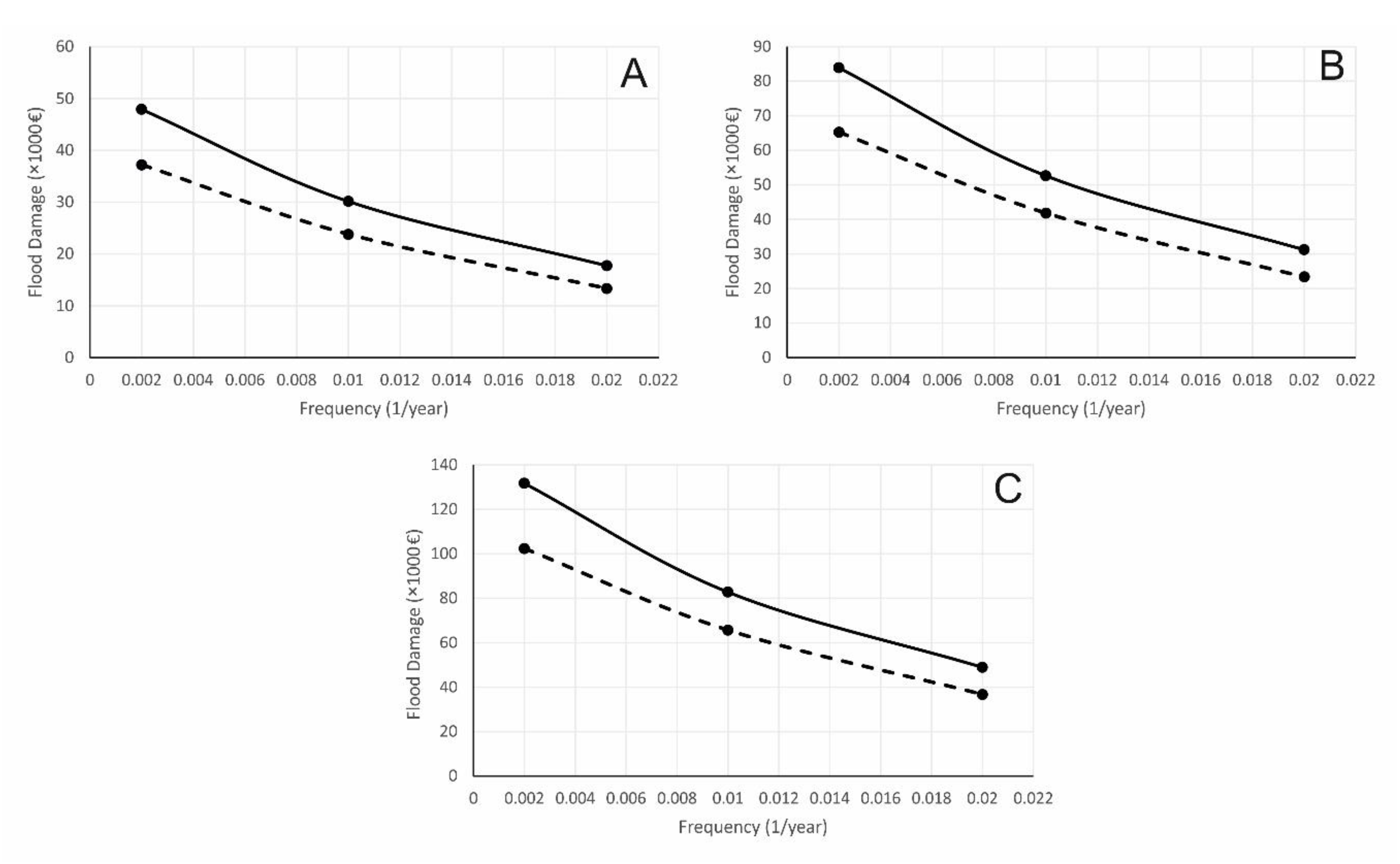
Finally, regarding the influence of the topographic relationship between the main floor of the houses and their surrounding land in the EAD estimation, results showed a clear reduction in the EAD value (Figure 8) regardless of the content, the structure or the combination of both. Thus, taking into account the damages associated with floods for a 50, 100, and 500 year return period, the EAD values were reduced by a percentage of over 22%. Specifically, for the whole structure and content of the dwellings, the EAD value for Navaluenga town was reduced from €132,000 to €102,500.
4. Discussion
Uncertainty in the estimation of damage associated with floods is a recurring subject addressed in this type of analysis [18,38]. This is due to the important variations observed and shown by different studies (e.g., References [39,40,41]) in terms of estimating damages. However, the complete elimination of uncertainty in flood damage estimation seems to be an impossible task, and this is partly due to the multiple sources of uncertainty linked to these analyses.
With regard to the damage estimation and making the issue more complex, there is no unanimity in the attribution of weights or influences on the uncertainty of the different sources linked to estimation, but it may be considered that there is a set of variables that constitute the greatest source of uncertainty. This set of variables can include the correct estimate of the flow frequency distribution function (which determines the magnitude and relative frequency of flooding in the territory), the flow depth, the damage models and the curves or magnitude–damage functions.
The first of the aforementioned variables, the correct estimation of the flow frequency distribution function, is recognized as one of the main sources of uncertainty in the damage estimation associated with floods (e.g., Reference [16,42]). Ballesteros–Cánovas et al. [41], in the town of Navaluenga (taken as a practical case study in the present study) affirmed that the percentage of uncertainty in flood damage estimation (associated with a correct estimate of the flow frequency law) in this town was above 40%. In this study, the flow frequency distribution function was first estimated using the data series of the gauging station, and this frequency law was later improved by the use of non–systematic information linked to dendro–geomorphological analyses. The uncertainty associated with this variable was much higher than other sources of uncertainty considered, such as the calibration of the hydrodynamic model, or the damage model used [41].
However, correct calibration of the hydrodynamic model should control and improve the estimation of flow depths, and this variable is considered essential in the uncertainty analysis in de Moel and Aerts’ [39] research. In their study, these authors associated variations of 10 cm in the flow depth with close to 6% variations in the flood damage estimation. This percentage was not negligible if multiple factors affecting the correct estimate of flow depths (quality and spatial resolution of the digital elevation model and land use model, for instance) were taken into account. The influence of the damage model used has also been considered a main source of uncertainty in flood damage estimation. Thus, Wagenaar et al. [43] calculated that the uncertainty associated with the use of different damage models (HIS–SSM for the Netherlands; HAZUS–MH in USA; FLEMO in Germany; Multi-Coloured Manual in UK; Rhine Atlas in Germany too; and others), all of them based on the concept of unit lost method, can be assigned an order of magnitude from 2 to 5. These authors identified this high uncertainty in the use of different damage models with the fact that these models were based on data related to a limited number of flood events. According to Thieken et al. [19], flood damage data are rarely collected systematically. In such a way, this limited number of events does not represent the multiple causative factors and particular characteristics of other floods or territories. This consideration is very important, and will affect the entire set of damage models or magnitude–damage functions, due to the near impossibility of such models or functions being used to replicate the assessment of flood damage in other locations, where both the features of the floods (flow depth, water velocities, solid load, response time, etc.) and the socioeconomic characteristics of the population can vary significantly. Additionally, linked to the damage model, Chinh et al. [44] estimated the uncertainty associated with this variable (in a study carried out in Vietnam) to be between 10% and 20% for damage to the structures of houses and between 8% and 15% for the content. However, these authors concluded that the uncertainty linked to hazard estimation may have been double that linked to the damage model.
On the other hand, Saint–Geours et al. [41] learned from their research that the main component of the uncertainty in estimating flood damage in houses is linked to the damage model used (a magnitude–damage curve in this case). In this study, the sensitivity index of the damage estimation model associated with the magnitude–damage function had a value of 0.78, compared to 0.22 linked to the flow frequency law. These results differed from those obtained for economic activities, where the main source of uncertainty was associated with the correct application of the flow frequency law.
All of the above show the variability of results related to the identification of the main uncertainty component in the flood damage estimation. The topographic variable (the height of the main floor and surrounding land) analysed in the present study was not considered in any of the cases, at least independently; Saint–Geours et al. [41] did seem to take it into account in their flood exposure model. This model particularly included land uses and their relation to economic activities, showing that their sensitivity index (0.03) was really insignificant and within the total estimation model of economic losses for houses compared to those mentioned above.
However, in no case was the direct influence of the topographic variable (difference in height between the main floor of the house and surrounding land) analysed in the estimation of flood damages in housing. As was shown in the present study, this variable determines the percentage of losses assigned to each dwelling, and the uncertainty introduced in the results reached similar levels to those pointed out by other authors for different variables. In addition, it is important to note that this variable influences the behaviour of other variables commonly used in flood damage estimation: flow depth and hazard models, flood exposure models, etc.
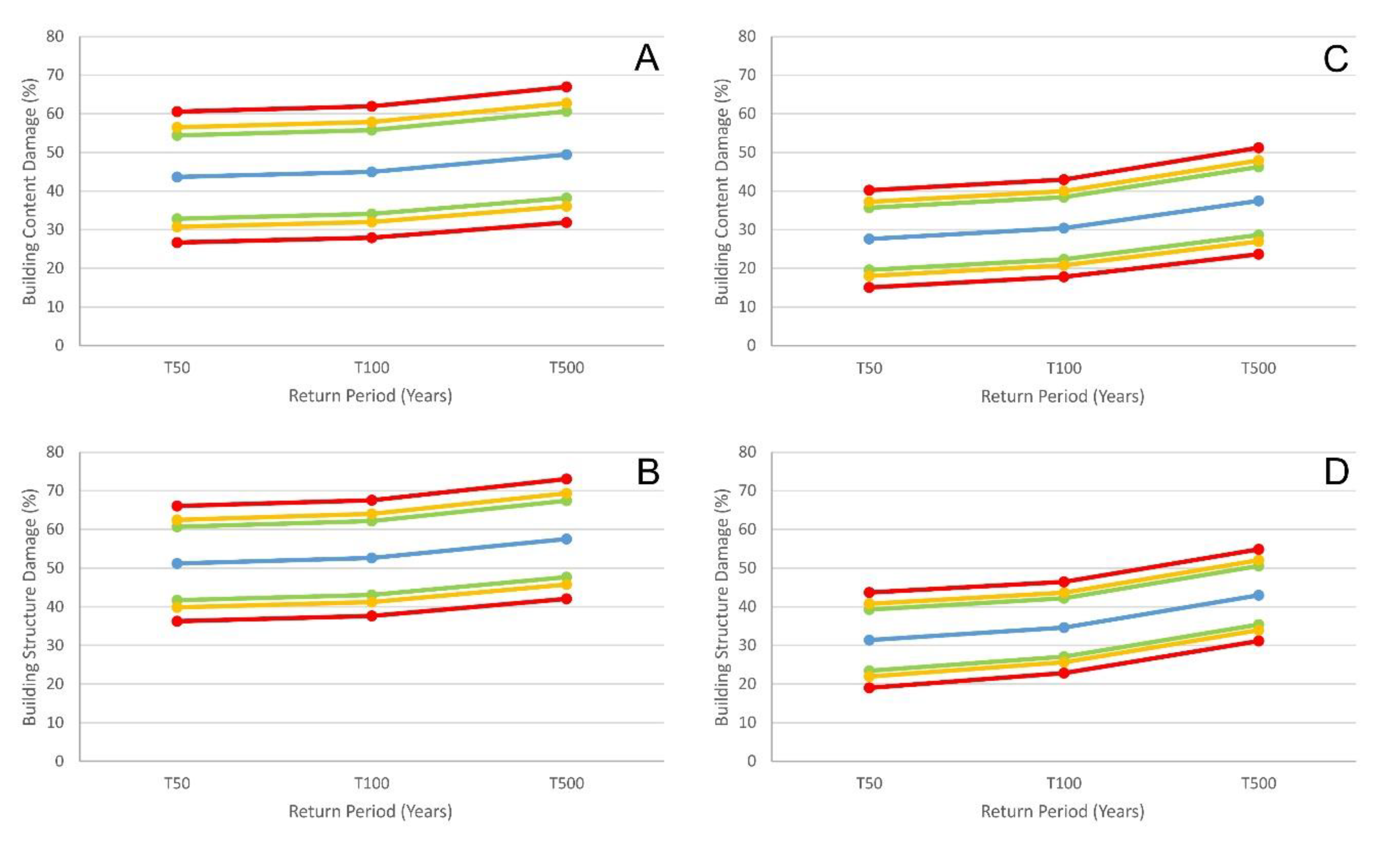
The assessment of economic damage due to flooding, or the variation in damage rate when considering the topographic relationship between the main floor of a house and the surrounding land, also implies uncertainty. This uncertainty is mainly associated with the damage model (magnitude–damage function) used. As we have seen, different models associate different damage rates to the same water depth value. The use of all considered magnitude–damage functions allows the calculation of an average economic damage value (%) associated with each flood return period, as well as the estimation of the confidence intervals (90%, 95% and 99%) related to those average damage values. The results of this analysis are shown in Figure 9, which shows the general reduction of damage rates when considering the topographic relationship between the main floor of a house and the surrounding land.
The uncertainty in average damage value was very similar regardless of the consideration of the topographic relationship between the main floor of the house and the surrounding land. In both cases, the uncertainty was slightly higher for the 50 year return period. When we considered the 90% confidence interval, the uncertainty in the estimation of the average value of flood damage ranged from 20% to 30%. This uncertainty reached a value of up to 45% (damage rate = 27.64 ± 12.58) when we considered the 99% confidence interval and a 50 year return period. These uncertainty values indicated a significant variability in the results depending on the model (magnitude–damage function) used, and reaffirmed the need for the development of detailed magnitude–damage functions at a local scale (as opposed to regional) for a correct estimate of economic damage due to flooding [21].
Furthermore, as the difference in height between the main floor of houses and the surrounding land is a variable that is independent of the damage model used (magnitude–damage function), the errors associated with this variable are independent as well. For this reason, the benefits of using a specific magnitude–damage function of a location (which takes into account the socio–economic conditions of the area) can disappear against the error introduced by this variable.
It should be noted that the influence of the variable that relates the height of the main floor of a house to the elevation in the surrounding land is not constant and independent of the value thereof. This influence is maximised in average values of flow depths (in the order of 0.2–0.6 m), which could be more frequently related to housing. In major flood depths, the influence of the analysed variable is also important; in flow depths above 1.5–2 m (the least common in urban areas where housing is located) the "height of main floor–surrounding land" relationship begins to have a lower impact. This is because the expected damages associated with these flow depths will be so serious (including the risk of collapse of structures) that they are usually associated with poorly developed urban areas.
The effect of the variable that relates the height of the main floor of the house to the surrounding land with respect to flood management and its mitigation measures can be raised. According to the field work carried out in the present study, the most commonly observed situation is one in which there is an over–elevation of the main floor. Therefore, although this may be a local effect not easily extrapolated to other locations, the most common result was the over–estimation of the economic damages linked to flood events when applying the classical methods. As a consequence, this over–estimation of the economic losses will affect the cost–benefit analyses linked to projects for the implementation of flood risk mitigation measures, extending to flood management by the persons and authorities responsible.
The dominant model of over–elevation has been considered previously, as a value of 0.3 m [45] was proposed to reduce the uncertainty in flood damage estimation analysis at regional or national scales. However, that general value may be not appropriate for local assessments, as our results pointed out. For Navaluenga, average over–elevation values ranged from 0.26 m for USACE Type II housing to 1.51 m for USACE Type I housing, with a general average value (independent from housing type) of 0.75 m. In general, in houses with basements, the over–elevation was higher. These differences highlight the variability associated with local construction models and the necessary estimation of the topographic relationship between the first floor and the surrounding land where local assessment will be carried out.
Finally, it must be noted that the results cannot be considered homogeneous, and they show that the construction model of houses will have a decisive influence on the economic losses linked to the different scenarios considered. Type of housing and building style (existence of a significant number of over– or under–elevated houses) can lead to the results regarding the percentage of flood damage differing greatly from those shown here. Thus, the applicability of the results obtained in the present assessment to other regions may be difficult, and more analysis of the relationship of flood damage and the topographic relationship between the height of the main floor and the surrounding land is necessary. However, even taking this into account, the results shown in the present study highlight the need to consider this variable in order to obtain estimates of economic damage that are closer to reality.
5. Conclusions
The correct estimation of damages (direct tangible losses) associated with floods is an essential aspect of efficient flood risk management. Moreover, the influence of DEM quality, the correct and precise inclusion of the buildings in the DSM used as the basis of hydrodynamic models, improvement in the estimation of the flow frequency law, calibration of hydrodynamic models for a correct flow depth estimation, implementation of different damage models, the development of specific magnitude–damage functions that take into account the socio–economic characteristics of the study area, etc. are all variables that have an influence on the estimation of flood damages, with the uncertainty associated with them being subject to study. However, no studies previously carried out have analysed the influence of the topographic relationship between the height of the main floor in dwellings and the surrounding land on flood damage estimation.
To analyse the behaviour and influence of this variable in flood damage estimation, 28 magnitude–damage functions of different types were considered. As expected, in all cases, a correlation was observed between the damage estimation trend (compared to non–consideration of this variable) and the topographic scenario proposed. It was alos noted that the influence of the variable was not homogeneous for the entire range of flow depth values analysed in the magnitude–damage functions. This influence on the flow depth range was maximal between 0.2 and 0.6 m and progressively decreased to below 10% in relation to flow depths of around 2 m or more.
For a real scenario, and using the magnitude–damage functions proposed by the USACE in the town of Navaluenga (Spain), an average over–estimation of more than 30% was obtained of the economic damages associated with floods with return periods of 50, 100 and 500 years. These percentages were not homogeneous and varied depending on the type of residential building and on the structure or content of the dwelling. Thus, in the case of one–storey houses with basements, the reduction in flood losses was maximal, reaching values between 55% and 60% for the structure and content of the house. By incorporating these variations in the economic damage estimation commonly used in the cost–benefit analysis of risk mitigation measures (EAD value of the town of Navaluenga), the over–elevation of the topographic height of the main floor in houses with regard to the surrounding land represented a 22.5% reduction in the EAD estimation.
All the data shown above helped us to determine that the variable “topographic relationship between the main floor of houses and the surrounding land” is one of the main sources of uncertainty in the estimation of flood damage in houses, similarly to others such as the correct determination of the flow frequency law, flow depth or damage model. It seems, therefore, that its consideration is essential for a proper estimation of economic losses due to floods, in the design and implementation of flood risk mitigation measure projects and for the general purpose of comprehensive flood risk management.
Author Contributions
All authors have a significant contribution to final version of the paper. Conceptualization, J.G.; Flood damage models analysis, N.B.; Writing—original draft, J.G.; Writing—review & editing, all authors. All authors have read and agreed to the published version of the manuscript.
Funding
This research was funded by the project DRAINAGE, CGL2017–83546–C3–R (MINEICO/AEI/FEDER, UE), and it is specifically part of the assessments carried out under the coverage of the sub–project DRAINAGE–3–R (CGL2017–83546–C3–3–R).
Acknowledgments
The authors would like to thank to Andrés Díez–Herrero (Geological Survey of Spain, IGME) for his constructive comments and help in conceptualizing the manuscript; and to Jose M. Bodoque and Estefanía Aroca (University of Castilla–La Mancha, Spain) for their flow depth data at Navaluenga town.
Conflicts of Interest
The authors declare no conflict of interest.
References
- Centre for Research on the Epidemiology of Disasters. The International Disaster Database. Available online: http://emdat.be/emdat_db/ (accessed on 15 July 2019).
- Munich RE. NatCatSERVICE Database. Available online: https://natcatservice.munichre.com/ (accessed on 17 July 2019).
- Ward, P.J.; Jongman, B.; Sperna Weiland, F.C.; Bouwman, A.; Van Beek, R.; Bierkens, M.; Ligtvoet, W.; Winsemius, H.C. Assessing flood risk at the global scale: Model setup, results, and sensitivity. Environ. Res. Lett. 2013, 8, 044019. [Google Scholar] [CrossRef]
- Visser, H.; Bouwman, A.; Petersen, A.; Ligtvoet, W. A Statistical Study of Weather–Related Disasters: Past, Present and Future; PBL Netherlands Environmental Assessment Agency: The Hague, The Netherlands, 2012; p. 87. [Google Scholar]
- De Moel, H.; Jongman, B.; Kreibich, H.; Merz, B.; Penning-Rowsell, E.; Ward, P.J. Flood risk assessments at different spatial scales. Mitig. Adapt. Strateg. Glob. Chang. 2015, 20, 865–890. [Google Scholar] [CrossRef] [PubMed] [Green Version]
- Sayers, P.; Lamb, R.; Panzeri, M.; Bowman, H.; Hall, J.; Horritt, M.; Penning-Rowsell, E. Believe it or not? The challenge of validating large scale probabilistic risk models. In Proceedings of the Floodrisk2016, Lyon, France, 17–21 October 2016; p. 11004. [Google Scholar] [CrossRef] [Green Version]
- Kourgialas, N.N.; Karatzas, G.P. Flood management and a GIS modelling method to assess flood–hazard areas—A case study. Hydrol. Sci. J. 2011, 56, 212–225. [Google Scholar] [CrossRef]
- Zhao, G.; Pang, B.; Xu, Z.; Yue, J.; Tu, T. Mapping flood susceptibility in mountainous areas on a national scale in China. Sci. Total Environ. 2018, 615, 1133–1142. [Google Scholar] [CrossRef] [PubMed]
- Pinto Santos, P.; Reis, E.; Pereira, S.; Santos, M. A flood susceptibility model at the national scale based on multicriteria analysis. Sci. Total Environ. 2019, 667, 325–337. [Google Scholar] [CrossRef]
- Winsemius, H.C.; Van Beek, R.; Jongman, B.; Ward, P.J.; Bouwman, A. A framework for global river flood risk assessments. Hydrol. Earth Syst. Sci. 2013, 17, 1871–1892. [Google Scholar] [CrossRef] [Green Version]
- Wilson, M.; Bates, P.; Alsdorf, D.; Forsbert, B.; Horritt, M.; Melack, J.; Frappart, F.; Famiglietti, J. Modeling largescale inundation of Amazonian seasonally flooded wetlands. Geophys. Res. Lett. 2007, 34, L15404. [Google Scholar] [CrossRef] [Green Version]
- Biancamaria, S.; Bates, P.D.; Boone, A.; Mognard, N.M. Large–scale coupled hydrologic and hydraulic modelling of the Ob River in Siberia. J. Hydrol. 2009, 379, 136–150. [Google Scholar] [CrossRef] [Green Version]
- Tang, J.C.S.; Vongvisessomjai, S.; Sahasakmontri, K. Estimation of flood damage cost for Bangkok. Water Resour. Manag. 1992, 6, 47–56. [Google Scholar] [CrossRef]
- Kreibich, H.; Seifert, I.; Merz, B.; Thieken, A.H. Development of flemocs—A new model for the estimation of flood losses in the commercial sector. Hydrol. Sci. J. 2010, 55, 1302–1314. [Google Scholar] [CrossRef]
- Merz, B.; Kreibich, H.; Schwarze, R.; Thieken, A. Review article ‘Assessment of economic flood damage’. Nat. Hazards Earth Syst. Sci. 2010, 10, 1697–1724. [Google Scholar] [CrossRef]
- Merz, B.; Hall, J.; Disse, M.; Schumann, A. Fluvial flood risk management in a changing world. Nat. Hazards Earth Syst. Sci. 2010, 10, 509–527. [Google Scholar] [CrossRef] [Green Version]
- Ernst, J.; Dewals, B.J.; Detrembleur, S.; Archambeau, P.; Erpicum, S.; Pirotton, M. Micro–scale flood risk analysis based on detailed 2D hydraulic modelling and high resolution geographic data. Nat. Hazards 2010, 55, 181–209. [Google Scholar] [CrossRef]
- Merz, B.; Kreibich, H.; Thieken, A.; Schmidtke, R. Estimation uncertainty of direct monetary flood damage to buildings. Nat. Hazards Earth Syst. Sci. 2004, 4, 153–163. [Google Scholar] [CrossRef] [Green Version]
- Thieken, A.H.; Müller, M.; Kreibich, H.; Merz, B. Flood damage and influencing factors: New insights from the August 2002 flood in Germany. Water Resour. Res. 2005, 41, W12430. [Google Scholar] [CrossRef]
- Soetanto, R.; Proverbs, D.G. Impact of flood characteristics on damage caused to UK domestic properties: The perceptions of building surveyors. Struct. Surv. 2004, 22, 95–104. [Google Scholar] [CrossRef] [Green Version]
- Garrote, J.; Alvarenga, F.M.; Díez-Herrero, A. Quantification of flash flood economic risk using ultra–detailed stage–damage functions and 2–D hydraulic models. J. Hydrol. 2016, 541, 611–625. [Google Scholar] [CrossRef]
- Horritt, M.S.; Bates, P.D. Effects of spatial resolution on a raster based model of flood flow. J. Hydrol. 2001, 253, 239–249. [Google Scholar] [CrossRef]
- Nicholas, A.P.; Walling, D.E. Modelling flood hydraulics and overbank deposition on river floodplains. Earth Surf. Proc. Land. 1997, 22, 59–77. [Google Scholar] [CrossRef]
- Horritt, M.S.; Bates, P.D. Predicting floodplain inundation: Rasted–based modelling versus the finite–element approach. Hydrol. Process. 2001, 15, 825–842. [Google Scholar] [CrossRef]
- Casas, M.A.; Benito, G.; Thorndycraft, V.R.; Rico, M.T. The topographic data source of digital terrain models as a key element in the accuracy of hydraulic flood modelling. Earth Surf. Proc. Land. 2006, 31, 444–456. [Google Scholar] [CrossRef]
- Bates, P.D.; De Roo, A.P.J. A simple raster–based model for flood inundation simulation. J. Hydrol. 2000, 236, 54–77. [Google Scholar] [CrossRef]
- Shen, D.; Qian, T.; Chen, W.; Chi, Y.; Wang, J. A Quantitative Flood–Related Building Damage Evaluation Method Using Airborne LiDAR Data and 2–D Hydraulic Model. Water 2019, 11, 987. [Google Scholar] [CrossRef] [Green Version]
- Bodoque, J.M.; Guardiola–Albert, C.; Aroca–Jimenez, E.; Eguibar, M.A.; Martinez–Chenoll, M.L. Flood damage analysis: First floor elevation uncertainty resulting from LiDAR derived digital surface models. Remote Sens. 2016, 8, 604. [Google Scholar] [CrossRef] [Green Version]
- Arrighi, C.; Campo, L. Effects of digital terrain model uncertainties on high resolution urban flood damage assessment. J. Flood Risk Manag. 2019, e12530. [Google Scholar] [CrossRef] [Green Version]
- Bermúdez, M.; Zischg, A.P. Sensitivity of flood loss estimates to building representation and flow depth attribution methods in micro–scale flood modelling. Nat. Hazards 2018, 92, 1633. [Google Scholar] [CrossRef] [Green Version]
- Garrote-Revilla, J.; Díez-Herrero, A.; Aroca-Jiménez, E.; Bodoque, J.M.; Bernal, N.; Martins, L.R. The relationship between the variables “main floor of houses with respect to their urban surroundings” and models for the estimation of economic losses owing to floods. In Interdisciplinarity in Practice and in Research on Society and the Environment: Joint Paths towards Risk Analysis, Proceedings of the SRA–E–Iberian Chapter (SRA–E–I) Conference, Toledo, Spain, 6–7 September 2018; Amérigo, M., García, J.A., Gaspar, R., Luís, S., Eds.; Ediciones de la Universidad de Castilla–La Mancha: Toledo, Spain, 2018; Volume 27811, pp. 111–112. [Google Scholar]
- USACE. Economic Guidance Memorandum (EGM) 01–03, Generic Depth–Damage Relationships; USACE: Washington, DC, USA, 2000; p. 11. [Google Scholar]
- USACE. Economic Guidance Memorandum (EGM) 04–01, Generic Depth–Damage Relationships for Residential Structures with Basements; USACE: Washington, DC, USA, 2003; p. 17. [Google Scholar]
- Van Der Sande, C. River Flood Damage Assessment Using IKONOS Imagery; European Commission, Joint Research Centre, Space Applications Institute (SAI): Ispra, Italy, 2001; p. 86. [Google Scholar]
- Salazar Galán, S.A. Metodología Para el Análisis y la Reducción del Riesgo de Inundaciones: Aplicación en la Rambla del Poyo (Valencia) Usando Medidas de “Retención de Agua en el Territorio”. Ph.D. Thesis, Polytechnic University of Valencia, Valencia, Spain, 2013. [Google Scholar]
- Huizinga, J.; De Moel, H.; Szewczyk, W. Global Flood Depth–Damage Functions: Methodology and the Database with Guidelines; Joint Research Centre: Luxembourg, 2017; p. 114. [Google Scholar] [CrossRef]
- Bellos, B.; Tsakiris, G. Comparing Various Methods of Building Representation for 2D Flood Modelling In Built–Up Areas. Water Resour. Manag. 2015, 29, 379–397. [Google Scholar] [CrossRef]
- Merz, B.; Thieken, A. Flood risk curves and uncertainty bounds. Nat. Hazards 2009, 51, 437–458. [Google Scholar] [CrossRef]
- De Moel, H.; Aerts, J.C.J.H. Effect of uncertainty in land use, damage models and inundation depth on flood damage estimates. Nat. Hazards 2011, 58, 407–425. [Google Scholar] [CrossRef] [Green Version]
- Ballesteros–Cánovas, J.A.; Sánchez–Silva, M.; Bodoque, J.M.; Díez–Herrero, A. An Integrated Approach to Flood Risk Management: A Case Study of Navaluenga (Central Spain). Water Resour. Manag. 2013, 27, 3051–3069. [Google Scholar] [CrossRef] [Green Version]
- Saint–Geours, N.; Grelot, F.; Bailly, J.S.; Lavergne, C. Ranking sources of uncertainty in flood damage modelling: A case study on the cost–benefit analysis of a flood mitigation project in the Orb Delta, France. J. Flood Risk Manag. 2015, 8, 161–176. [Google Scholar] [CrossRef]
- Apel, H.; Thieken, A.H.; Merz, B.; Blöschl, G. Flood risk assessment and associated uncertainty. Nat. Hazards Earth Syst. Sci. 2004, 4, 295–308. [Google Scholar] [CrossRef]
- Wagenaar, D.J.; de Bruijn, K.M.; Bouwer, L.M.; de Moel, H. Uncertainty in flood damage estimates and its potential effect on investment decisions. Nat. Hazards Earth Syst. Sci. 2016, 16, 1–14. [Google Scholar] [CrossRef] [Green Version]
- Chinh, D.T.; Dung, N.V.; Gain, A.K.; Kreibich, H. Flood Loss Models and Risk Analysis for Private Households in Can Tho City, Vietnam. Water 2017, 9, 313. [Google Scholar] [CrossRef]
- Maqsood, T.; Wehner, M.; Ryu, H.; Edwards, M.; Dale, K.; Miller, V. GAR15 Vulnerability Functions: Reporting on the UNISDR/GA SE Asian Regional Workshop on Structural Vulnerability Models for the GAR Global Risk Assessment; Geoscience Australia: Canberra, Australia, 2014; p. 74. [Google Scholar] [CrossRef]
Figure 1.
Magnitude–damage models used. The models are classified in relation to their consideration of content, structure, or content + structure.
Figure 1.
Magnitude–damage models used. The models are classified in relation to their consideration of content, structure, or content + structure.

Figure 2.
Examples of houses with topographic over– and under–elevation with respect to the surrounding land.
Figure 2.
Examples of houses with topographic over– and under–elevation with respect to the surrounding land.

Figure 3.
Flow depth estimation in the houses considering topographic over– or under–elevation with respect to the surrounding land, in the case of residential buildings both with and without a basement.
Figure 3.
Flow depth estimation in the houses considering topographic over– or under–elevation with respect to the surrounding land, in the case of residential buildings both with and without a basement.

Figure 4.
Switzerland magnitude–damage model for river flooding, showing its characteristic staggered shape.
Figure 4.
Switzerland magnitude–damage model for river flooding, showing its characteristic staggered shape.

Figure 5.
River flooding economic damage change (%) by considering topographic over– and under–elevation of buildings from magnitude–damage models of the Czech Republic (A), Australia–Content (B), HKV–Content (C), USA–Type IV–Content (D), Pajares de Pedraza–V2P (E) and Pollo Ravine–Type II (F).
Figure 5.
River flooding economic damage change (%) by considering topographic over– and under–elevation of buildings from magnitude–damage models of the Czech Republic (A), Australia–Content (B), HKV–Content (C), USA–Type IV–Content (D), Pajares de Pedraza–V2P (E) and Pollo Ravine–Type II (F).

Figure 6.
Examples of the effect of the magnitude–damage model graphic shape in the economic damage change evolution when considering the topographic over– or under–elevation of building main floor. The examples are related to magnitude–damage models of Switzerland (A), United Kingdom (B) and Germany (C).

Figure 7.
Navaluenga building classification according to USACE building types; and examples of flood economic damage change by considering the topographic over– and under–elevation of houses against its surrounding land.
Figure 7.
Navaluenga building classification according to USACE building types; and examples of flood economic damage change by considering the topographic over– and under–elevation of houses against its surrounding land.

Figure 8.
Damage–frequency curves for Navaluenga town considering content (A), structure (B) or content + structure (C). The solid line represents the original results, and the dashed line represents the results linked to the consideration of the topographic difference between the main floor of housing and surrounding land.

Figure 9.
Average values and confidence intervals (90%: green line; 95%: yellow line; 99%: red line) for flood economic damage (%) at Navaluenga (Spain) from all magnitude–damage functions considered. Results not taking into account the topographic relationship between the main floor of the house and the surrounding land (A,B), and taking the topographic relationship into account (C,D).


Table 1.
List of magnitude–damage models and their main characteristics.
| Magnitude–Damage Function | Proposed Working Scale | Considered Elements | Potential Damage | Curve Shape | Maximum Flow Depth | Maximum Damage (%) | Flooding Type | ||||
|---|---|---|---|---|---|---|---|---|---|---|---|
| Content | Structure | Combined | Basement | € | % | ||||||
| HKV Consultants–Structure | Meso–scale | x | x | asymptotic at 5 m | 6 m | 100 | River flooding | ||||
| HKV Consultants–Content | Meso–scale | x | x | asymptotic at 5 m | 6 m | 100 | River flooding | ||||
| Australia–Structure | Macro–scale | x | x | no asymptotic | 3 m | 41 | River flooding | ||||
| Australia–Content | Macro–scale | x | x | asymptotic at 1.8 m | 3 m | 89 | River flooding | ||||
| Spain (Pajares Pedraza)–V1P | Micro–scale | x | x | no asymptotic | 2 m | 100 | Flash Flood | ||||
| Spain (Pajares Pedraza)–V1O | Micro–scale | x | x | no asymptotic | 2 m | 100 | Flash Flood | ||||
| Spain (Pajares Pedraza)–V2P | Micro–scale | x | x | no asymptotic | 2 m | 100 | Flash Flood | ||||
| Spain (Pajares Pedraza)–V2O | Micro–scale | x | x | no asymptotic | 2 m | 100 | Flash Flood | ||||
| USACE–Type I–Content | Macro–scale | x | x | x | asymptotic at 3.4 m | 5 m | 39.1 | River flooding | |||
| USACE–Type I–Structure | Macro–scale | x | x | x | asymptotic at 3.4 m | 5 m | 81.1 | River flooding | |||
| USACE–Type II–Content | Macro–scale | x | x | asymptotic at 4 m | 5 m | 40 | River flooding | ||||
| USACE–Type II–Structure | Macro–scale | x | x | no asymptotic | 5 m | 80.7 | River flooding | ||||
| USACE–Type III–Content | Macro–scale | x | x | x | no asymptotic | 5 m | 52.6 | River flooding | |||
| USACE–Type III–Structure | Macro–scale | x | x | x | asymptotic at 4.6 m | 5 m | 76.4 | River flooding | |||
| USACE–Type IV–Content | Macro–scale | x | x | no asymptotic | 5 m | 37.2 | River flooding | ||||
| USACE–Type IV–Structure | Macro–scale | x | x | no asymptotic | 5 m | 69.2 | River flooding | ||||
| Europe–Content | Macro–scale | x | x | no asymptotic | 6 m | 100 | River flooding | ||||
| Switzerland–Content | Meso–scale | x | x | asymptotic at 3 m | 6 m | 64 | River flooding | ||||
| Czech Republic–Content | Meso–scale | x | x | no asymptotic | 6 m | 42 | River flooding | ||||
| Netherlands–Content | Macro–scale | x | x | asymptotic at 5 m | 6 m | 58 | River flooding | ||||
| Germany–Content | Macro–scale | x | x | no asymptotic | 6 m | 84 | River flooding | ||||
| United Kingdom–Content | Macro–scale | x | x | asymptotic at 3 m | 6 m | 100 | River flooding | ||||
| Spain (Poyo Ravine)–Single–family, no garage (Type I) | Micro–scale | x | x | x | asymptotic at 1.3 m | 2 m | 100 | Flash Flood | |||
| Spain (Poyo Ravine)–Single–family, garage ground floor (Type II) | Micro–scale | x | x | x | asymptotic at 1.3 m | 2 m | 100 | Flash Flood | |||
| Spain (Poyo Ravine)–Single–family, garage basement (Type III) | Micro–scale | x | x | x | x | asymptotic at 1.2 m | 2 m | 100 | Flash Flood | ||
| Spain (Poyo Ravine)–Multi–family, no garage (Type IV) | Micro–scale | x | x | x | asymptotic at 1.2 m | 2 m | 100 | Flash Flood | |||
| Spain (Poyo Ravine)–Multi–family, garage ground floor (Type V) | Micro–scale | x | x | x | asymptotic at 1.4 m | 2 m | 100 | Flash Flood | |||
| Spain (Poyo Ravine)–Multi–family, garage basement (Type VI) | Micro–scale | x | x | x | x | asymptotic at 1.4 m | 2 m | 100 | Flash Flood | ||
Table 2.
Navaluenga flood economic damage reduction considering topographic over–or under–elevation of houses.
Table 2.
Navaluenga flood economic damage reduction considering topographic over–or under–elevation of houses.
| Economic Damage Reduction (%) | ||||||
|---|---|---|---|---|---|---|
| Housing Type 1 | T50 | T100 | T500 | |||
| Content | Structure | Content | Structure | Content | Structure | |
| Type I | 61.34 | 67.81 | 54.82 | 59.17 | 50.20 | 44.73 |
| Type II | 17.55 | 18.22 | 14.57 | 15.44 | 12.46 | 13.19 |
| Type III | 34.26 | 42.78 | 33.77 | 41.26 | 30.47 | 34.55 |
| Type IV | 24.36 | 23.48 | 22.12 | 21.48 | 18.64 | 18.25 |
1 Type I: one storey with basement; Type II: one storey without basement; Type III: two or more storeys with basement; Type IV: two or more storeys without basement.
© 2020 by the authors. Licensee MDPI, Basel, Switzerland. This article is an open access article distributed under the terms and conditions of the Creative Commons Attribution (CC BY) license (http://creativecommons.org/licenses/by/4.0/).
Share and Cite
MDPI and ACS Style
Garrote, J.; Bernal, N. On the Influence of the Main Floor Layout of Buildings in Economic Flood Risk Assessment: Results from Central Spain. Water 2020, 12, 670. https://doi.org/10.3390/w12030670
AMA Style
Garrote J, Bernal N. On the Influence of the Main Floor Layout of Buildings in Economic Flood Risk Assessment: Results from Central Spain. Water. 2020; 12(3):670. https://doi.org/10.3390/w12030670
Chicago/Turabian StyleGarrote, Julio, and Nestor Bernal. 2020. "On the Influence of the Main Floor Layout of Buildings in Economic Flood Risk Assessment: Results from Central Spain" Water 12, no. 3: 670. https://doi.org/10.3390/w12030670
Note that from the first issue of 2016, this journal uses article numbers instead of page numbers. See further details here.