Article

Investigation into the Effects of Climate Change on Reference Evapotranspiration Using the HadCM3 and LARS-WG

1
Agriculture Faculty, Malayer University, Malayer 6571995863, Iran
2
College of Electrical Engineering and New Energy, China Three Gorges University, Yichang 443002, China
3
Hubei Provincial Key Laboratory for Operation and Control of Cascaded Hydropower Station, China Three Gorges University, Yichang 443002, China
4
State Key Laboratory of Hydrology-Water Resources and Hydraulic Engineering, Hohai University, Nanjing 210098, China
5
School of Technology, Ilia State University, 0162 Tbilisi, Georgia
6
School of Hydropower and Information Engineering, Huazhong University of Science & Technology, Wuhan 430074, China
*
Authors to whom correspondence should be addressed.
Water 2020, 12(3), 666; https://doi.org/10.3390/w12030666
Submission received: 2 October 2019 / Revised: 15 November 2019 / Accepted: 23 February 2020 / Published: 1 March 2020
(This article belongs to the Special Issue Effects of Climate Change on Water Resources)

Abstract

:
This study evaluates the effect of climate change on reference evapotranspiration (ET0), which is one of the most important variables in water resources management and irrigation scheduling. For this purpose, daily weather data of 30 Iranian weather stations from 1981 and 2010 were used. The HadCM3 statistical model was applied to report the output subscale of LARS-WG and to predict the weather information by A1B, A2, and B1 scenarios in three periods: 2011–2045, 2046–2079, and 2080–2113. The ET0 values were estimated by the Ref-ET software. The results indicated that the ET0 will rise from 2011 to 2113 approximately in all stations under three scenarios. The ET0 changes percentages in the A1B scenario during three periods from 2011 to 2113 were found to be 0.98%, 5.18%, and 12.17% compared to base period, respectively, while for the B1 scenario, they were calculated as 0.67%, 4.07%, and 6.61% and for the A2 scenario, they were observed as 0.59%, 5.35%, and 9.38%, respectively. Thus, the highest increase of the ET0 will happen from 2080 to 2113 under the A1B scenario; however, the lowest will occur between 2046 and 2079 under the B1 scenario. Furthermore, the assessment of uncertainty in the ET0 calculated by the different scenarios showed that the ET0 predicted under the A2 scenario was more reliable than the others. The spatial distribution of the ET0 showed that the highest ET0 amount in all scenarios belonged to the southeast and the west of the studied area. The most noticeable point of the results was that the ET0 differs from one scenario to another and from a period to another.

1. Introduction

Changes in the climate system balance increase the importance of evaluation of climate change effects on hydrological parameters. On the other hand, climate prediction is necessary for water resources sustainable management [1,2,3,4]. By creating General Circulation Models (GCM), climate conditions can be assessed for long-time scales. However, the output of these models does not have enough spatial and temporal accuracy to study the effect of climate change on hydrological systems. Thus, applying suitable downscaling models can improve the results of climate change studies [5,6,7,8]. LARS-WG, as one of the downscaling models, is used for the simulation of climate information under current and future circumstances. The superiority of this model over others such as the SDSM downscaling model was reported [9,10,11]. In the literature, several studies demonstrated the successful prediction of different climatic variables using LARS-WG, including the prediction of temperature and precipitation, extreme floods for a medium-sized basin in Northeastern China, air temperature in the Brazos Headwaters Basin of Texas, precipitation in the Koshi River Basin of Nepal, and drought in Iran [10,11,12,13,14,15,16,17]. More studies have reported that the performance of the LARS-WG model was effective in downscaling GCM outputs due to representing future weather characteristics by updating the model parameters based on the outputs of GCMs [18].
Hassan et al. [18] applied SDSM and LARS-WG for simulating and downscaling of rainfall and temperature of Peninsular Malaysia. They found that LARS-WG as a suitable tool for quantifying the climate change effect. Kai Duan and Yadong Mei [19] utilized the LARS-WG for simulating and downscaling of rainfall of China and found that LARS-WG provided better accuracy in modeling extreme indices. Chen et al. [20] reported the successful application of LARS-WG in downscaling and predicting daily precipitation, maximum temperature, and minimum temperature in Sudan. Hashmi et al. [21] stimulated and downscaled well the extreme precipitation events of Clutha River catchment in New Zealand using the LARS-WG model. Etemadi et al. [22] reported the superiority of the LARS-WG model over the SDSM model in the downscaling of temperature in an aquatic ecosystem. The successful applications of the LARS-WG model compelled the authors to choose this model and the other main reason for the selection of the LARS-WG model, compared to the other models in this study, is that it incorporates different GCM outputs to better handle their uncertainties.
Evapotranspiration (ET) as an important hydrological parameter is affected by weather variables such as temperature, relative humidity, wind speed, solar radiation, and so on. Subsequently, climate change can influence ET as confirmed by the previous investigations [23,24,25]. Harmsen et al. [26] evaluated the effect of climate change on the reference ET in a study in 2009 and he found decreasing crop yields in Puerto Rico under different scenarios. They declared that the crop yield will decrease under all scenarios. Guo et al. [27] showed an increase in wheat yields in the North China Plain. In another study, climate change did not have a significant effect on wheat ET [28]. However, the survey of Remrova and Cislerova [29] indicated that climatic change will significantly affect in terms of ET up to the year 2100. A similar result was reported by Nepal [30] that the ET is sensitive to climate change. Abdolhosseini et al. [31] evaluated the effect of climate change on potential ET (ET0) and illustrated that the ET0 values in future periods will decline significantly compared to the past period. On the contrary, the results of Rajabi and Babakhani [32] indicated that in all five stations, located in the west of Iran, the ET0 values will increase from 2011 to 2099. Tiegang et al. [33] by investigating the future ET0 trend in the southwest of China declared that there was a spatially increasing trend between 1960 and 2010 from northeast to southeast.
Previous studies in the literature have illustrated the successful application of LARS-WG in the prediction of some weather variables over Iran [34,35]; for instance, assessments of climate change impact on water resources and forecasting drought during the next years [16,36]. It is a well-known fact that future trends of ET0 changes are different in different climates. Moreover, there is a lack of investigation on how the variability of ET0 is affected by climate change in regions with different climates. So, the main purpose of this study is the evaluation of the ET0 amount in future time horizons under different climatic scenarios in Iran. In this study, the effect of climate change on the ET0 of Iran will be examined. To downscale climate change based on one of the GCM sub-models (called HadCM3), the LARS-WG will be used as a tool for generating weather statistically. LARS-WG downscales the climate variables according to HadCM3 under three scenarios of emissions, namely, A2, B1, and A1B. The results of the present investigation can be applied in water resources management of the country particularly in the agriculture sector.

2. Materials and Methods

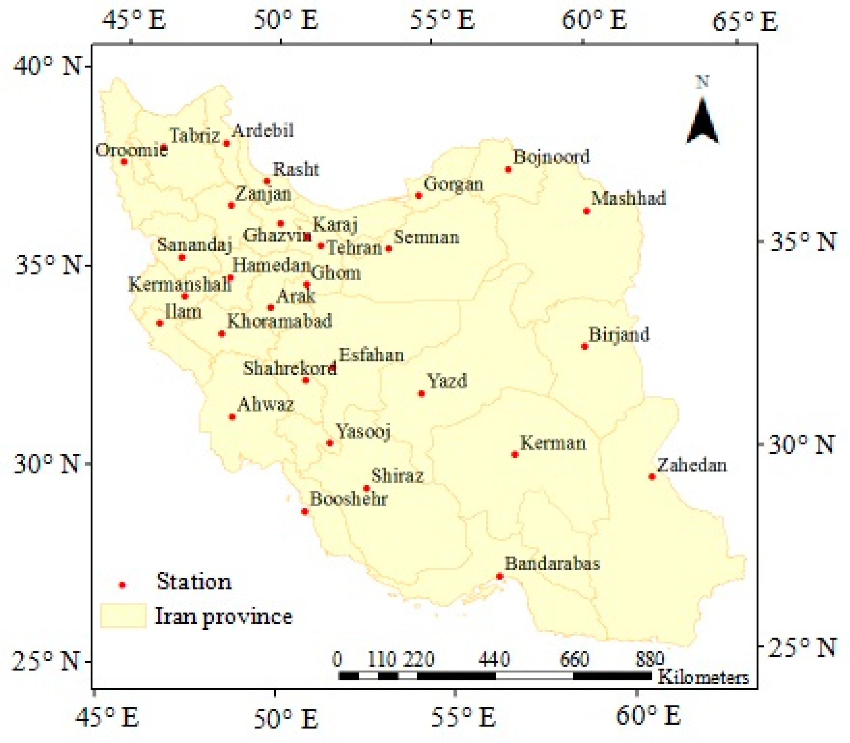
Iran, with an area of more than 1,648,000 km2, is located between 25°00′ N and 38°39′ N latitudes and 44°00′ E and 63°25′ E longitudes. In this study, to assess the effect of climate change on the ET0, daily data records collected from 30 synoptic stations during a period of 30 years (1981–2010) were used. The primary reason for selecting these stations is the suitable quality of data and the same time period. Moreover, the selected stations are mostly located in different climates and represent a very good spatial distribution over the region. The geographical location and distribution of the stations are shown in Figure 1. Due to the weather condition, the north part of Iran is the main agricultural producing region. Regarding this fact, the number of weather stations in this area is more than in other areas.
Since the estimation of ET0 requires the meteorological variables, first of all, weather parameters were calculated for the future period using the LARS-WG model. For this purpose, by considering variables of minimum temperature (Tmin), maximum temperature (Tmax), solar radiation (RS), and precipitation for each station from 1981–2010 (base period), the LARS-WG model was calibrated. In other words, the value of each weather variable including Tmin, Tmax, RS, and precipitation was simulated. Then, the values of observed and simulated variables were compared with each other. Normal root mean square error (NRMSE) and correlation of coefficient (r) were utilized for the comparison of observed and predicted values.
N R M S E = [ 1 n i = 1 n ( X Y ) 2 ] 0.5 X ¯
r = ( i = 1 n ( X X ¯ ) ( Y Y ¯ ) ) 2 i = 1 n ( X X ¯ ) 2 ( Y Y ¯ ) 2
where X and Y are the observed and simulated values, respectively; X ¯ and Y ¯ are the average of X and Y and n is the total number of data.
After making sure of the accuracy of the model, the same parameters were forecasted in the future. For this purpose, three scenarios, A1B, A2, and B1, were considered. The assumption in the scenario of B1 depends on an endurable world, fast changes in economic constructions, development of human rights equality, and a care to protect the environment. Considering this assumption, greenhouse gas circulation (GGC) may be controlled and for industries (e.g., factories), a program for pollutant controlling will be applied. The assumption in the A1B scenario depends on a wealthy world with a fast economic development (3% for each year), a decrease in population (27% for each year), the fast development of technology, cultural, and economic convergence and a fundamental decrement in regional differences. The assumption in the A2 scenario depends on the existence of a separate world. Various cultural identities in different regions of the world increase differences in the world and reduce international cooperation [32]. So the weather parameters were predicted for three 34-year periods, 2011–2045, 2046–2079, and 2080–2113, under different scenarios. Due to the fact that there is a time limitation on LARS-WG in predicting weather variables, for filling gap among defined periods was considered three 34-year periods.
In the second step, the amount of ET0 was calculated by the Hargreaves–Samani (HS) method in the Ref-ET software. Due to the fact that high accuracy and less meteorological data are needed in the application of the HS, previous studies have recommended this method in Iran [32,37,38]. For instance, Raziei and Pereira [39] reported that the HS method is an appropriate alternative in the estimation of ET0 for all climatic regions of Iran. In the absence of sunshine, relative humidity, and wind speed data, ET0 can be estimated by the HG method which uses the minimum and maximum temperatures bearing in mind the effect of latitude as follows:
E T 0 = 0.0023 R a ( T + 17.8 ) T R
where ET0 is the potential evapotranspiration (mm), T is the average temperature (°C), TR is the difference between the minimum and maximum temperatures (°C), and Ra is extraterrestrial radiation (MJm−2day−1). For estimating the ET0, the Ref-ET software was applied. The accuracy of the Ref-ET software in estimating the ET0 is reported in several investigations [40,41]. Finally, considering the weather parameters during the next years, the amount of the ET0 was predicted for the periods of 2011–2045, 2046–2079, and 2080–2113 under each scenario.
The ET0 changes ( Δ E T 0 ) in the future were calculated using Equation (4) to compare with the base period (1981–2010).
Δ E T 0 = E T 0 ( i , j ) E T 0 ( b ) E T 0 ( b ) × 100
where E T 0 ( i , j ) is the ET0 value in the ith period i and the j scenario, E T 0 ( b ) is the ET0 in the base period.
Due to the fact that wheat is the most important cereal grain all over the world, thus after calculating the ET0, the net irrigation requirement of this crop during the future years was estimated. For this purpose, initially with considering the ET0 and the crop coefficient (the FAO table) the wheat evapotranspiration (ETC) was calculated (Equation (5)). Afterward, the wheat net irrigation requirement (IRC) was determined based on the effective rainfall (Re) and the ETC using Equation (7). It is noticeable that the FAO dependable rain method was used for estimating the Re (Equation (6)).
E T C = E T 0 × k C
i f P 70 m m t h e n Re = 0.8 × P 24 , i f P 70 m m t h e n Re = 0.6 × P 10
I R C = E T C Re
where, P is the precipitation value in millimeters, ETC is the wheat evapotranspiration (mm), the Kc is the wheat crop coefficient, which was obtained from the recommended table of the FAO.
Finally, the spatial distribution of the daily ET0 was drawn using the inverse distance weighted (IDW) method in ArcGIS 10.3. The IDW interpolation explicitly assumes that features that are close to one another are more alike than those that are farther apart. The use of the IDW method was recommended for data with short changes in the range [42]. Besides, the IDW has shown better accuracy in comparison to the Kriging method in interpolation when there is a limited number of data [43].
Moreover, it is undeniable that there is uncertainty in each prediction process. Therefore, in this study for the assessment of uncertainty in the prediction of the ET0 under different scenarios, the boxplot charts were applied [44]. For this purpose, the average ET0 predicted during different months under each scenario was assessed.

3. Results

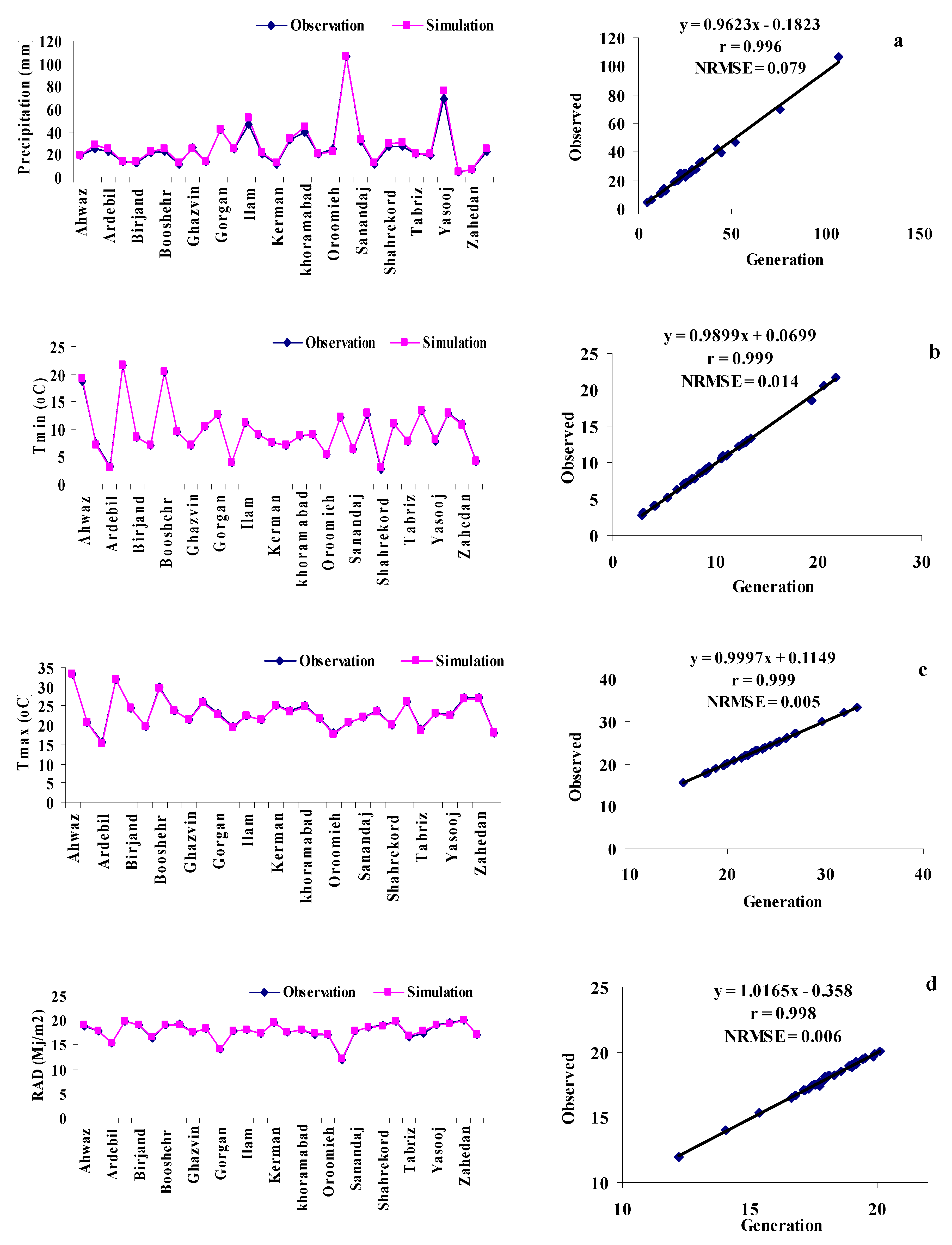
As was mentioned in the material and method, the calibration of the LARS-WG model was done using the weather parameters (Tmin, Tmax, RS, and precipitation) in the base period. Figure 2 shows the results of the model calibration. This figure was prepared based on the values of observed and estimated for each parameter in the base period. It is necessary to be known that the average calibration results were reported for each station in Figure 2.
Based on the results of Figure 2, the evaluation of model accuracy in the prediction of weather parameters indicates that the ability of the model in predicting the Tmax is better than the other parameters. It can be seen from the figure that the accuracy of the model in the calibration step for the Tmax has the lowest NRMSE (0.005) and the highest r (0.999). In contrast, the ability of the model in simulation of the precipitation is worse than the others. The amount of NRMSE and r for the precipitation are 0.014 and 0.999, respectively. Overlay, the comparison of statistical indexes indicates that the performance of the LARS-WG model in the calibration phase was suitable and reasonable.
After achieving confidence from the performance of the LARS-WG, the values of the ET
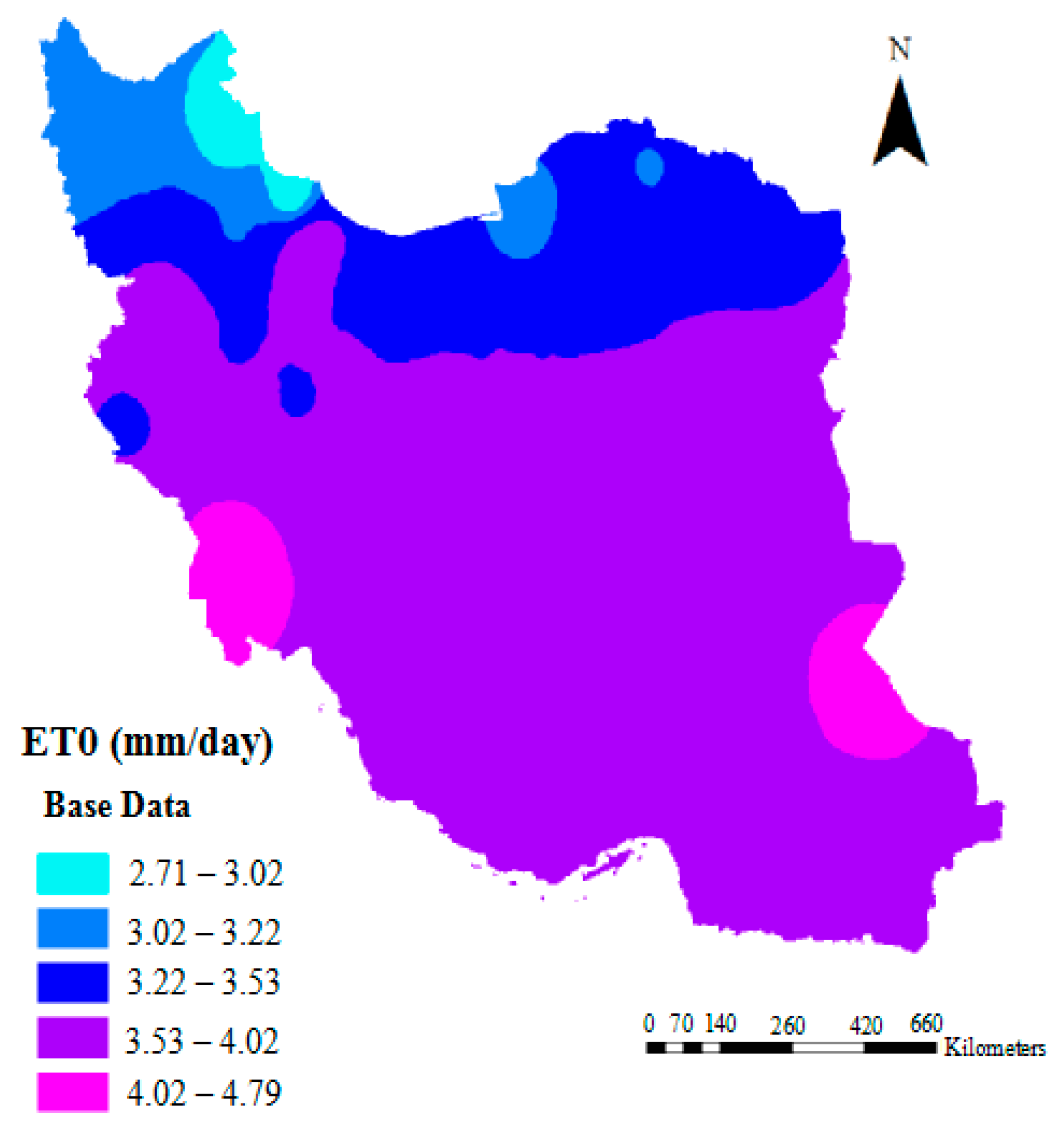
0 were calculated over the base period and then they were predicted for the future. Figure 3 displays the spatial distribution of the daily ET0 in the base period over Iran.
The result of Figure 3 shows that the ET0 values in the northern half of the country are less than the southern half. So that the ET0 ranges from 2.71 to 3.02 in the northern half while in the southern half, it varies from 3.53 to 4.79.
After the calibration stage, weather variables were predicted for the next years from 2011 to 2113 with three categories including 2011–2045, 2046–2079, and 2080–2113 under different scenarios. Table 1, Table 2, Table 3, Table 4, Table 5, Table 6, Table 7 and Table 8 show the percentage of the change of the ET0 values of each period compared to the base period (Equation (4)) for every station in different months. The zero values in some of the cells in the table mean that some changes are insignificant and trivial.
It can be inferred from Table 1 that the highest percentages indicate positive changes, by 77% (278 out of 360). In other words, for most stations, the ET0 amount will increase in most of the months. The same consequences are reported by Dinpashoh et al. [20]. The highest ET0 drop is observed in January and February, while other months will experience ET0 increase. According to Table 1, the maximum decrease will happen in November at the Tabriz station with −34.71% compared to the highest increase which is observed in June at the Kermanshah station with 7.98%.
Based on the results of Table 2, the number of negative changes of the ET0 for the 2011–2045 period under the A1B scenario decreased from 22% to 20% by using the A2 scenario. Similar to the results of scenario A1B, the highest decrease in ET0 belongs to November at the Tabriz station by a narrow margin. In contrast, the maximum increase in ET0 changes in scenario A1B is similar to the scenario A2, about 7.8%. The most noticeable point in Table 2 is that the ET0 changes percentage in August for all stations will rise, compared to August under scenario A1B. In general, the average ET0 change in Table 2 is 0.98% while it is 0.59% in Table 1. In other words, scenario A2 estimates more increases in the ET0.
The number of negative percentages of ET0 changes under the B1 scenario is more than the other scenarios during the same period. As can be seen from Table 3, 25% of ET0 changes are negative. In other words, ET0 changes in a large number of stations will increase in comparison to scenarios A1B and A2. Comparing the ET0 change percentages among stations, the maximum increase is 21.66% in March at the Bojnoord station. The highest decrease is similar to the results from scenarios A1B and A2.
Table 4 gives information about the change percentages of the ET0 from 2046 to 2079 in comparison with the base period under A1B scenario. It can be clearly seen from this table that there is an approximately increasing trend except for September at Semnan and November at Tabriz. Moreover, there are a higher proportion of positive change percentages in 2046–2079 than in the first 34-year period (2011–2045). In other words, the vast majority of changes in the second period is positive than the first period. The average change percentage of the ET0 in Table 4 is 5.34% and is more noticeable than the previous period. Comparing the monthly results of stations, the highest ET0 value is 13.62% and occurs in June at the Kermanshah station during the second 34-year period. However, considering the average of all the months, the maximum average ET0 change percentage is observed in the Oroomieh station.
According to the results of Table 5, it can be inferred that the average ET0 change percentage from 2046 to 2079 under the A2 scenario across all stations is 5.18%. In other words, there is a slight difference between the A2 and A1B scenarios throughout the second 34-year period. The maximum increase in ET0 over the whole period belongs to the Mashhad station with 8.58%. Similar to the previous results, the lowest ET0 change percentage is −32.35% in November at the Tabriz station. Looking in more detail indicates that the ET0 values will go down by 0.83% in the studied stations.
The data given in Table 6 indicate that the ET0 changes percentage under the B1 scenario is more than the other scenarios in the same period from 2046 to 2079. Based on the results of Table 6, the average ET0 change percentage is 4.07% across all stations. The more details of this table state that in 2.5% of the stations, the ET0 values have declined compared to the base period. The maximum and minimum ET0 change percentages are observed in June at Kermanshah and November at the Tabriz station, respectively. As a consequence, during the second 34-year period, the ET0 increase compared with the base period in the A1B scenario is more than the other scenarios and the A2 scenario is more than the B1 scenario.
The results of predicting ET0 from 2080 to 2113 under the A1B1 scenario in Table 7 indicate that the ET0 values will rise significantly compared to the base period. As can be seen from this table, the average ET0 change percentage is about 9.38%. Based on the information given, the highest increase percentage is 22.73% and seen in January at Arak station; however, considering the results of the whole months, the maximum ET0 will be observed in the Ardebil station. The most noticeable point of this table is that the greatest decrease in ET0 will occur in August at the Semnan station.
Examining the ET0 predicted for the 2080–2113 period under the A2 scenario shows that unlike previous periods, the ET0 value increased more than the A1B scenario. As can be seen from Table 8, the average ET0 changes percentage is 12.17%, which is completely different from the previous results. The highest increase is 141.88% and observed in November at the Hamedan station. In other words, there is no constant trend in the prediction of ET0 in the future under different scenarios. Moreover, the lowest ET0 value is 43.72% and will happen in March at the Hamedan station.
Table 9 gives information about the ET0 change during the third 34-year period from 2080 to 2113 by considering the B1 scenario. According to the results of Table 9, it is legalized that the ET0 values in this scenario are less than the previous two scenarios at the same period with a wide margin. In addition to this, the greatest increase in the ET0 is observed in April at the Ilam station, while the lowest growth is in November at the Tabriz station. The average ET0 changes percentage in Table 9 is 6.61%. In general, in this period, the ET0 increase in the A2 scenario will be more than the others. On the other hand, the ET0 value in the A1B will be more than the B1 scenario.
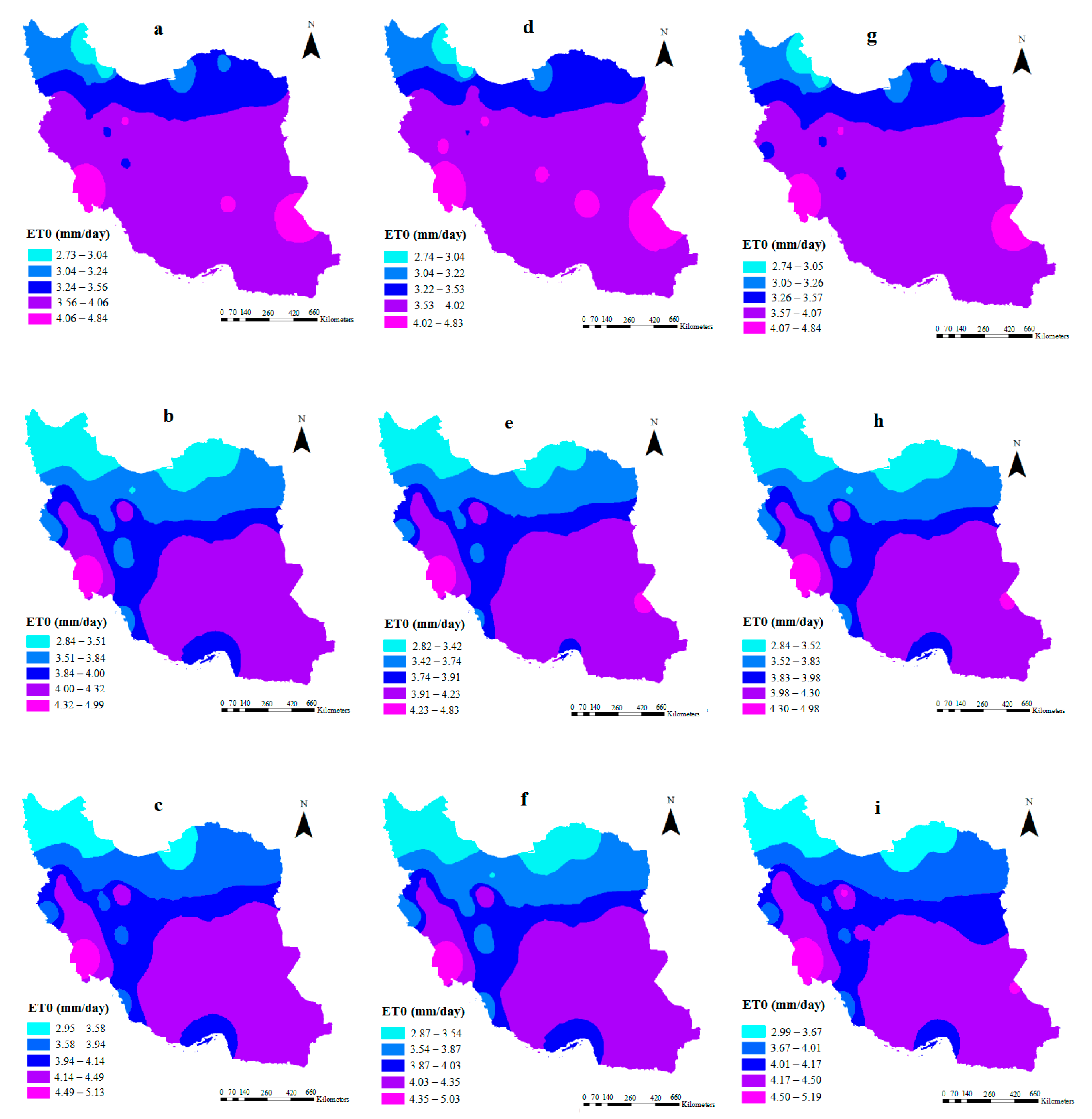
Figure 4 illustrates the spatial distribution of the ET0 predicted under different scenarios in the future. These maps are drawn into five categories. According to Figure 4, the ET0 values in the north half of country are less than the south half. This result is in line with Figure 3 (base period). The changing trend of the ET0 over the country in the first period is similar to the base timescale, however, there is a dramatic difference between the spatial distribution of the ET0 in the base period and the second and third periods. The highest ET0 amount in all maps belongs to the southeast and the west of the studied area. Due to the type of climate in these regions, these predictions seem reasonable.
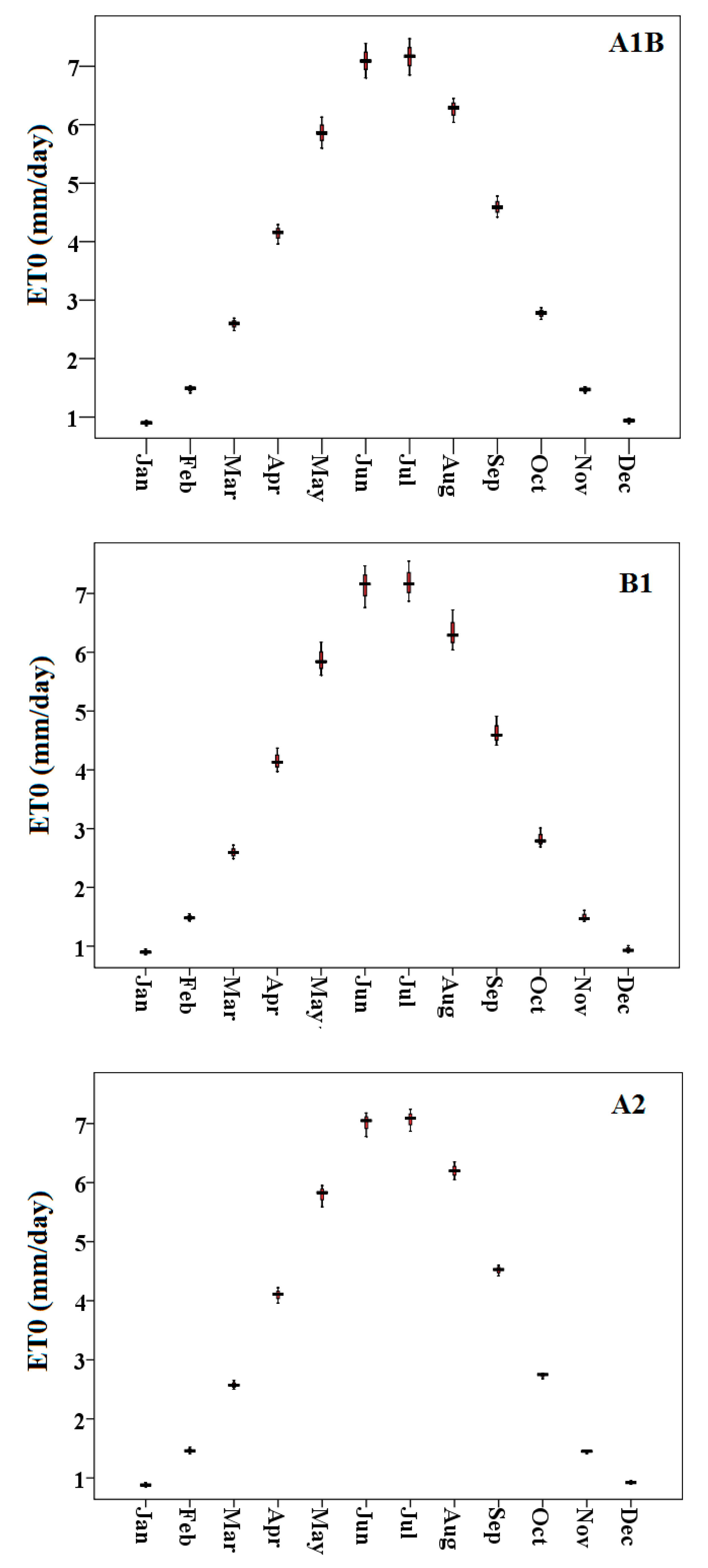
Uncertainty consequences of the ET0 predicted by the LARS-WG model under distinct scenarios are shown in Figure 5. The distance between the first and third quartile (height of boxplots) indicates amounts of uncertainty. For drawing these charts, the average ET0 predicted from 2011 to 2113 was used. As can be seen from Figure 5, the highest uncertainty in each of the three scenarios is observed between April and September, whereas the ET0 values at the beginning and end of the year experience the minimum uncertainty. In other words, the uncertainty in the ET0 of the mid-year is more than others. However, in January and December, there is a high certainty for the prediction of the ET0 in all the study scenarios. Comparing the results of each scenario in Figure 5 demonstrates that the certainty of the ET0 values in the A2 scenario is higher than the other scenarios. It seems to be crystal clear that the height of boxplots in the B1 and A1B scenarios is more than the A2 scenario.
Regarding this finding, the estimated ET0 under the A2 scenario is more reliable, considering the ET
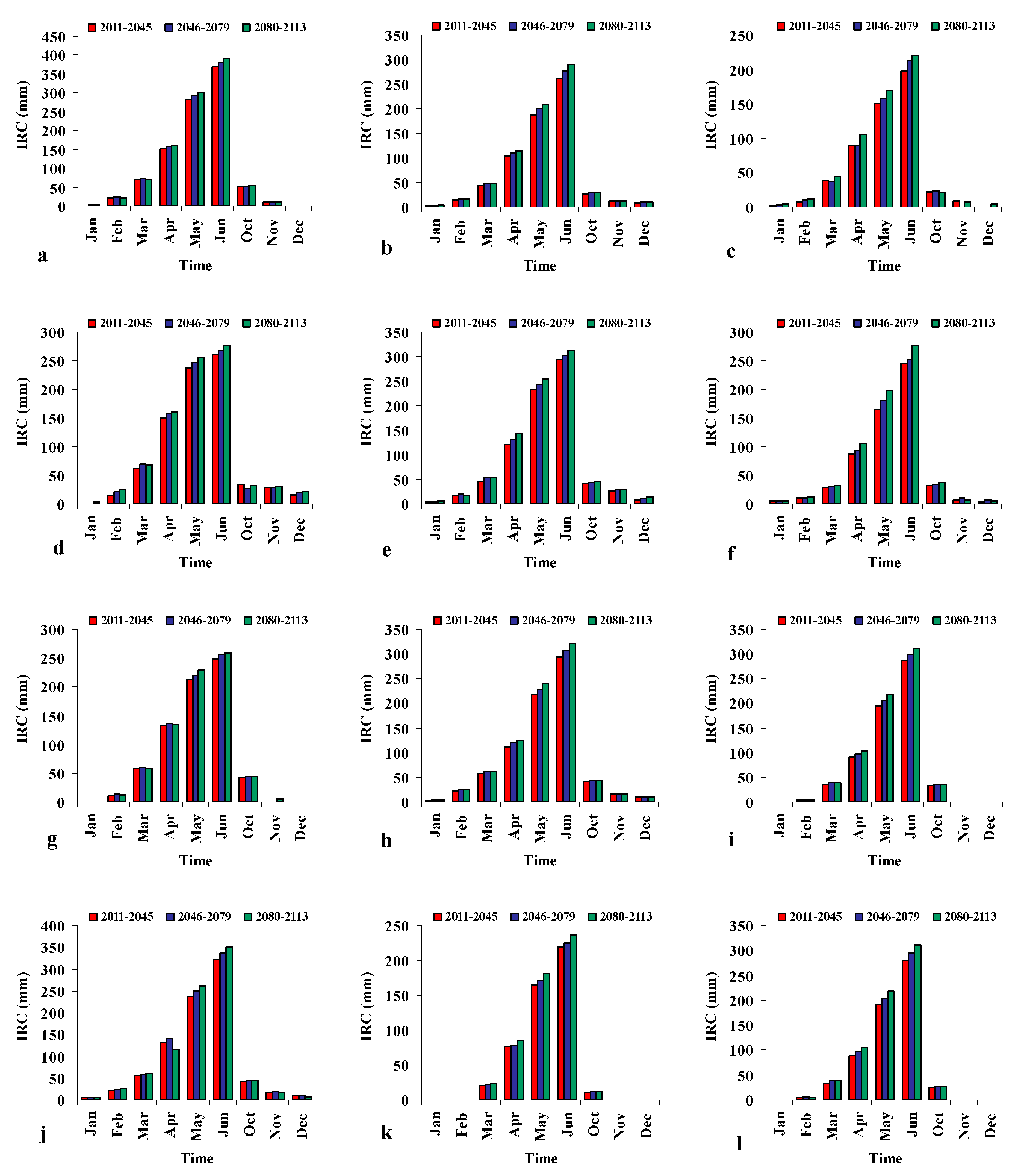
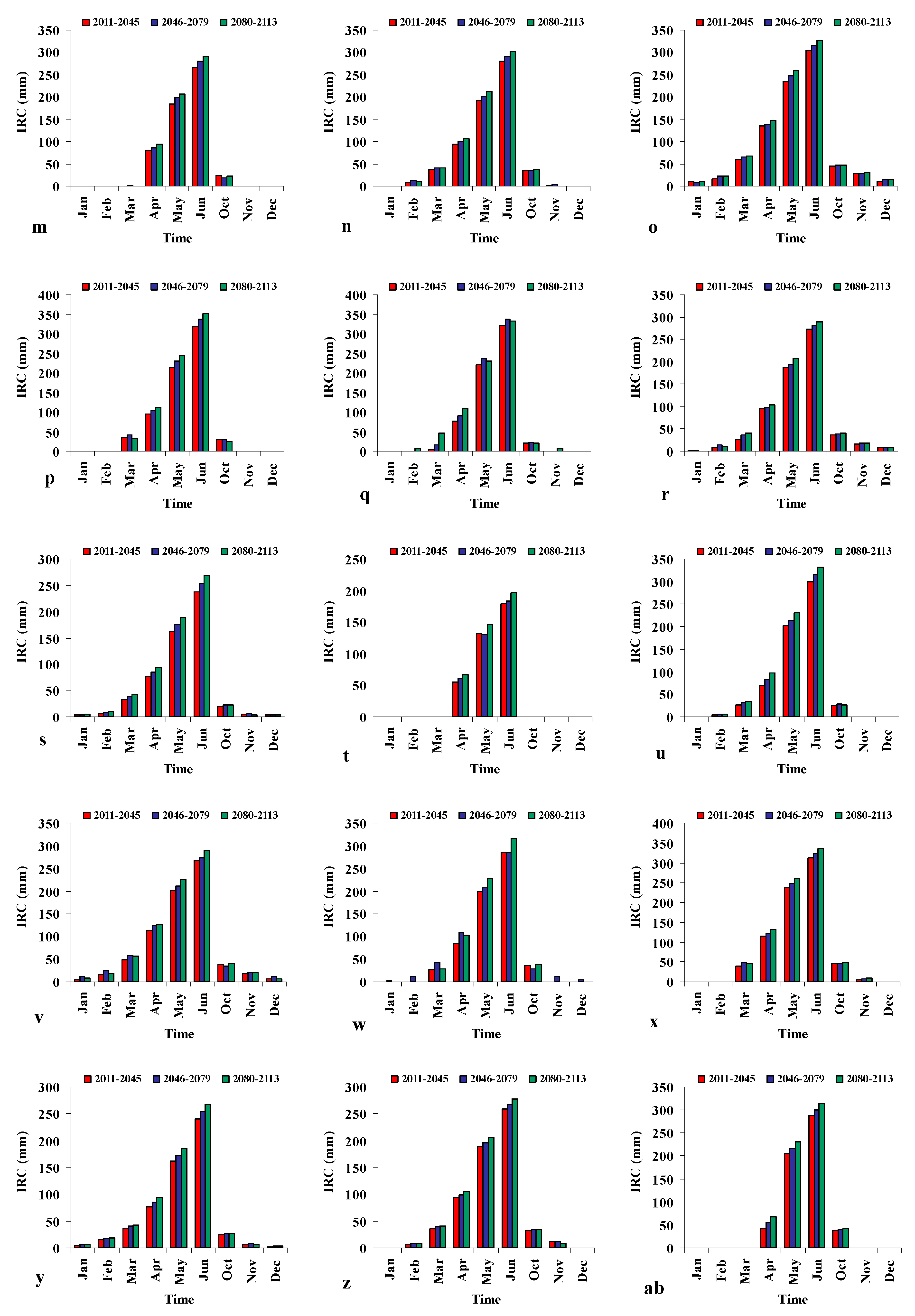
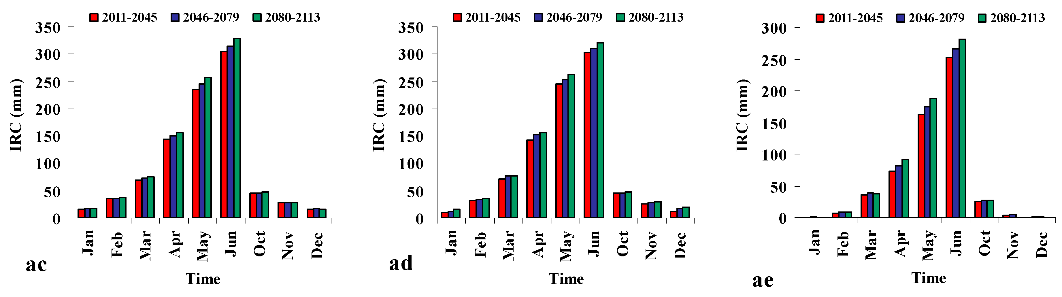
0 predicted under the A2 scenario for the future years and the effective rainfall (Equation (6)), the value of the net irrigation requirement of the wheat (IRC) as a major field crop was calculated (Equation (7)). Due to the fact that most of the wheat in Iran is cultivated in October and harvested in July [45], therefore the net irrigation requirement of the wheat during these months was estimated. Figure 6 indicates the IRC values from 2011 to 2013 under the A2 scenario as a reliable scenario.
As can be seen from Figure 6, there is a fluctuation in the IRC values during the growth period of wheat in all studied stations. However, it is noticeable that the highest amount of the IRC would occur in June in most stations. In other words, there is an upward trend in the amount of the IRC from January to June, compared to a downward trend between October and December. Furthermore, it seems to be crystal clear that the IRC values will increase from 2011 to 2013 in the vast majority of stations. On top of these, the maximum amount of the IR
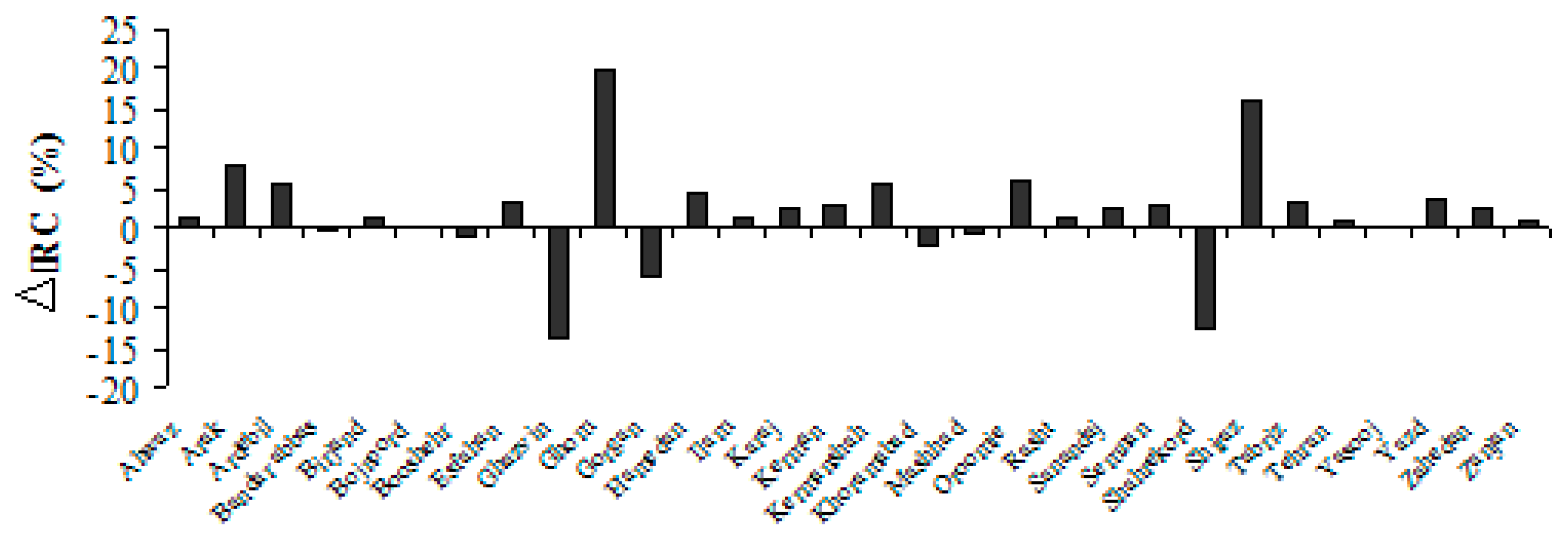
C is observed in Ahwaz, whereas the minimum amount is related to the Rasht station. In general, this figure can be worthwhile in water management of the agriculture sector, which could provide farmers a plan for managing irrigation in cultivating wheat. For comparing the change percentage of the net irrigation requirement of the wheat from the base period to the future, the values of the change percentage of the IRC for each station are shown in Figure 7.
According to the given information in Figure 7, it can be inferred that the vast majority of stations will experience the IRC increase in the next years to the base period. The highest increase would be observed in Ghom station by 19.74%. Whereas, in seven out of 30 studied stations (approximately 23 percent of stations), the amount of IRC might decrease in the future. The maximum drop belongs to Ghazvin by 13.74%.

4. Discussion

Due to the fact that the main purpose of calibration of each model is to find the accuracy and ability of the model in discovering a link between the dependent and independent variables, so the error statistics in this stage can state the trust degree of the model [46]. Following this hypothesis, the results of the calibration of the LARS-WG model illustrated that the highest and lowest accuracies of the model in prediction of weather variables in the base timescale belonged to the Tmax and the precipitation, respectively. In other words, the error statistics such as the correlation coefficient can mention the accuracy of the model in appearing the relation between parameters. For instance, the r-value in the prediction of all variables was more than 0.99, which can confirm that the model results are reliable with 99% probably. In the study of Hassan et al. [18], it is also reported that the LARS-WG fits observed air temperature better than other variables. Nover et al. [47] expressed that the prediction of the Tmax in LARS-WG has the highest accuracy. LARS-WG performance in predicting precipitation was acceptable in the investigation by Agarwal et al. [11], therefore, this is in line with the present study.
The prediction of the ET0 for the next years demonstrated that the ET0 values will go up from 2011 to 2113, approximately, for all stations under all three scenarios. This result is in line with the research by Rajabi and Babakhani [32] in Iran and Tiegang et al. [33] in China. In conclusion, the highest increase of the ET0 in the future over Iran will happen from 2080 to 2113 under the A1B scenario, while the lowest will be observed from 2046 to 2079 under the B1 scenario. Consequently, the most critical condition from the aspect of the ET0 is predicted for the A1B scenario. Rajabi and Babakhani [32] reported the same result. By studying the climate change effect on the ET0 changes in the west of Iran, they stated that the highest ET0 rise will happen in the A1B scenario. Comparing the ET0 predicted among studied stations indicated that in most cases the Tabriz station will experience an ET0 decrease in November. The investigation of Asakereh and Akbarzadeh [46] shows that the temperature changes of this station in November during the next years will decrease. Due to the fact that the ET0 changes depend on the temperature changes directly, the present result is in line with their study. It seems that for tackling the negative effects of the ET0 increase in the future, a change in the cropping pattern and cultivation crops with the lowest irrigation requirement can be a suitable solution for addressing the next issues. As Leng and Huang [48] mentioned that the planting pattern change can remedy the situation of negative impacts of climate change and subsequently increase the ET0.
The assessment of the spatial distribution of the ET0 showed that the rerated value in the northern half of the country is less than the southern half. Due to the fact that the northern areas of Iran are mountainous and the climate of the northern half is cooler than the southern half, these results are acceptable. One of its reasons can be the different temperatures of both regions. In the study of Babaeian et al. [45], it was declared that the air temperature of the southern half is higher than the northern half. Moreover, it can be seen from the ET0 values for the future that the ET0 will increase from 2011 to 2113 under three scenarios. The most noticeable is that the trend of the change of the ET0 in the second and third periods is pretty different from the first period. According to the temperature increase and precipitation decrease in Iran during the next years, which are predicted by Babaeian et al. [45], and the drought increase, predicted by Khazanedari et al. [16], it was found that providing for agricultural water requirements would be a serious crisis in near future. It is noticeable that there is uncertainty in each prediction, which can be because of the quality and quantity of data or the model structure [46]. Regarding this fact, evaluation of uncertainty in the results of each scenario in the prediction of the ET0 indicated that the ET0 predicted by the A2 scenario is more reliable than the others, which is reported in the investigation of Houghton et al. [49]. Following this finding, for evaluating one of the applications of the ET0 prediction in the agriculture sector, the net irrigation requirement of the wheat for the next decades was estimated. For this purpose, the future IRC values under the A2 scenario were compared with the base period. Due to the fact that the IRC is calculated based on the effective rainfall and the ETC (Equation (7)), thus a lot of variables influence the IRC. In other words, if there is a dramatic increase in the amount of precipitation the IRC would decline sharply. While, the increase of the ETC can be in parallel with the rise of the IRC. One of the main reasons for the IRC increase in the future can be the precipitation drop and an increase in air temperature, which has been mentioned in severe surveys [50]. According to the results of the calibration stage, which indicated that the accuracy of temperature predication was more than others, it can be stated that in the present study, the importance of air temperature on the ETC and subsequently the IRC seems to be more than other weather parameters. From the aspect of the decrease of the IRC of wheat during the next years, the same consequence has been reported in some studies [51], which is in line with the present investigation.

5. Conclusions

Applying LARS-WG in the simulation of weather variables showed that the accuracy of the model in the calibration step for the maximum temperature had the lowest error. Inversely, the ability of the model in estimating precipitation was less than the others. Examining the ET0 changes by different scenarios indicated that the ET0 will increase in the future; however, the most noticeable point was that the ET0 increase in the third period was more than the other two periods. The highest ET0 increase will happen from 2080 to 2113 under the A1B scenario, while the lowest will be observed from 2046 to 2079 under the B1 scenario. The spatial distribution of the ET0 illustrated that the ET0 values in the northern half of the country are less than the southern half. The highest ET0 amount in all scenarios was observed in the southeast and the west of the country. On top of these, the evaluation of uncertainty in the obtained results showed that the ET0 predicted under the A2 scenario was more reliable than the others. Moreover, there was a high uncertainty in the ET0 estimated for the warm months of the year. Following this point, the net irrigation requirement of the wheat, as a major crop, for the future years under the A2 scenario was estimated. According to the change’s percentage of the future net irrigation requirement of wheat to the base period, a decrease of the IRC was observed in 23% of the studied stations, compared to the IRC increase in 77% of stations. Consequently, the ability to provide agricultural water requirements could be a serious crisis in the near future in Iran.

Author Contributions

Formal analysis, M.B. and O.K.; methodology, O.K. and X.Y.; writing—original draft, M.B. and R.M.A.; supervision, R.F. and B.Z. All authors have read and agreed to the published version of the manuscript.

Acknowledgments

The authors gratefully acknowledge the financial support received from the Open Fund of the Hubei Provincial Key Laboratory for Operation and Control of Cascaded Hydropower Station in China Three Gorges University (No. 2019KJX02).

Conflicts of Interest

The authors declare no conflict of interest.

References

  1. Lee, C.-H.; Yeh, H.-F. Impact of Climate Change and Human Activities on Streamflow Variations Based on the Budyko Framework. Water 2019, 11, 2001. [Google Scholar] [CrossRef] [Green Version]
  2. Masud, M.B.; Ferdous, J.; Faramarzi, M. Projected Changes in Hydrological Variables in the Agricultural Region of Alberta, Canada. Water 2018, 10, 1810. [Google Scholar] [CrossRef] [Green Version]
  3. Destouni, G.; Prieto, C. Robust Assessment of Uncertain Freshwater Changes: The Case of Greece with Large Irrigation—And Climate-Driven Runoff Decrease. Water 2018, 10, 1645. [Google Scholar] [CrossRef] [Green Version]
  4. Adnan, R.M.; Liang, Z.; El-Shafie, A.; Zounemat-Kermani, M.; Kisi, O. Prediction of Suspended Sediment Load Using Data-Driven Models. Water 2019, 11, 2060. [Google Scholar] [CrossRef] [Green Version]
  5. Arshad, A.; Zhang, Z.; Zhang, W.; Gujree, I. Long-Term Perspective Changes in Crop Irrigation Requirement Caused by Climate and Agriculture Land Use Changes in Rechna Doab, Pakistan. Water 2019, 11, 1567. [Google Scholar] [CrossRef] [Green Version]
  6. Miao, Q.; Pan, B.; Wang, H.; Hsu, K.; Sorooshian, S. Improving Monsoon Precipitation Prediction Using Combined Convolutional and Long Short Term Memory Neural Network. Water 2019, 11, 977. [Google Scholar] [CrossRef] [Green Version]
  7. Dahm, R.; Bhardwaj, A.; Sperna Weiland, F.; Corzo, G.; Bouwer, L.M. A Temperature-Scaling Approach for Projecting Changes in Short Duration Rainfall Extremes from GCM Data. Water 2019, 11, 313. [Google Scholar] [CrossRef] [Green Version]
  8. Adnan, R.M.; Liang, Z.; Yuan, X.; Kisi, O.; Akhlaq, M.; Li, B. Comparison of LSSVR, M5RT, NF-GP, and NF-SC Models for Predictions of Hourly Wind Speed and Wind Power Based on Cross-Validation. Energies 2019, 12, 329. [Google Scholar] [CrossRef] [Green Version]
  9. Semenov, M.A.; Barrow, E.M. LARS-WG: A Stochastic Weather Generator for Use in Climate Impact Studies; Rothamsted Research: Hertfordshire, UK, 2002. [Google Scholar]
  10. Rajabi, A.; Sedghi, H.; Eslamian, S.; Musavi, H. Comparison of LARS-WG and SDSM downscaling models in Kermanshah (Iran). Ecol. Environ. Conserv. 2010, 16, 1–7. [Google Scholar]
  11. Adnan, R.M.; Liang, Z.; Trajkovic, S.; Zounemat-Kermani, M.; Li, B.; Kisi, O. Daily streamflow prediction using optimally pruned extreme learning machine. J. Hydrol. 2019, 577, 123981. [Google Scholar] [CrossRef]
  12. Karimi, S.; Karimi, S.; Yavari, A.R.; Niksokhan, M.H. Prediction of temperature and precipitation in Damavand Catchment in Iran by using LARS-WG in future. Earth Sci. 2015, 4, 95–100. [Google Scholar] [CrossRef] [Green Version]
  13. Awal, R.; Bayabil, H.; Fares, A. Analysis of potential future climate and climate Extremes in the Brazos Headwaters basin, Texas. Water 2016, 8, 603. [Google Scholar] [CrossRef] [Green Version]
  14. Agarwal, A.; Babel, M.S.; Maskey, S. Analysis of future precipitation in the Koshi river basin, Nepal. J. Hydrol. 2014, 513, 422–434. [Google Scholar] [CrossRef]
  15. Khazanedari, L.; Zabol Abbasi, F.; Ghandhari, S.; Kouhi, M.; Malbousi, S. Drought prediction in Iran during next 30 Years. In Proceedings of the 9th EMS Annual Meeting, 9th European Conference on Applications of Meteorology (ECAM), Toulouse, France, 28 September–2 October 2009. [Google Scholar]
  16. Qi, W.; Zhang, C.; Fu, G.; Zhou, H.; Liu, J. Quantifying uncertainties in extreme flood predictions under climate change for a medium-sized basin in Northeastern China. J. Hydrometeorol. 2016, 17, 3099–3112. [Google Scholar] [CrossRef]
  17. Adnan, R.M.; Liang, Z.; Heddam, S.; Zounemat-Kermani, M.; Kisi, O.; Li, B. Least square support vector machine and multivariate adaptive regression splines for streamflow prediction in mountainous basin using hydro-meteorological data as inputs. J. Hydrol. 2019, 124371. [Google Scholar] [CrossRef]
  18. Hassan, Z.; Shamsudin, S.; Harun, S. Application of SDSM and LARS-WG for simulating and downscaling of rainfall and temperature. Theor. Appl. Climatol. 2014, 116, 243–257. [Google Scholar] [CrossRef]
  19. Duan, K.; Mei, Y. A comparison study of three statistical downscaling methods and their model-averaging ensemble for precipitation downscaling in China. Theor. Appl. Climatol. 2014, 116, 707–719. [Google Scholar] [CrossRef]
  20. Chen, H.; Guo, J.; Zhang, Z.; Xu, C.Y. Prediction of temperature and precipitation in Sudan and South Sudan by using LARS-WG in future. Theor. Appl. Climatol. 2013, 113, 363–375. [Google Scholar] [CrossRef]
  21. Hashmi, M.Z.; Shamseldin, A.Y.; Melville, B.W. Comparison of SDSM and LARS-WG for simulation and downscaling of extreme precipitation events in a watershed. Stoch. Environ. Res. Risk Assess. 2011, 25, 475–484. [Google Scholar] [CrossRef]
  22. Etemadi, H.; Samadi, S.; Sharifikia, M. Uncertainty analysis of statistical downscaling models using general circulation model over an international wetland. Clim. Dyn. 2014, 42, 2899–2920. [Google Scholar] [CrossRef]
  23. Moses, O.; Hambira, W.L. Effects of climate change on evapotranspiration over the Okavango Delta water resources. Phys. Chem. Earth Parts A/B/C 2018, 105, 98–103. [Google Scholar] [CrossRef]
  24. Dinpashoh, Y.; Jahanbakhsh-Asl, S.; Rasouli, A.A.; Foroughi, M.; Singh, V.P. Impact of climate change on potential evapotranspiration (case study: West and NW of Iran). Theor. Appl. Climatol. 2019, 136, 185–201. [Google Scholar] [CrossRef]
  25. Adnan, R.M.; Malik, A.; Kumar, A.; Parmar, K.S.; Kisi, O. Pan evaporation modeling by three different neuro-fuzzy intelligent systems using climatic inputs. Arab. J. Geosci. 2019, 12, 606. [Google Scholar] [CrossRef]
  26. Harmsen, E.W.; Miller, N.L.; Schlegel, N.J.; Gonzalez, J.E. Seasonal climate change impacts on evapotranspiration, precipitation deficit and crop yield in Puerto Rico. Agric. Water Manag. 2009, 96, 1085–1095. [Google Scholar] [CrossRef]
  27. Guo, R.; Lin, Z.; Mo, X.; Yang, C. Responses of crop yield and water use efficiency to climate change in the North China Plain. Agric. Water Manag. 2010, 97, 1185–1194. [Google Scholar] [CrossRef]
  28. Bannayan, M.; Rezaei, E.E. Future production of rainfed wheat in Iran (Khorasan province): Climate change scenario analysis. Mitig. Adapt. Strateg. Glob. Chang. 2014, 19, 211–227. [Google Scholar] [CrossRef]
  29. Remrová, M.; Císlerová, M. Analysis of climate change effects on evapotranspiration in the watershed uhlířská in the Jizera mountains. Soil Water Res. 2010, 5, 28–38. [Google Scholar] [CrossRef] [Green Version]
  30. Nepal, S. Impacts of climate change on the hydrological regime of the Koshi river basin in the Himalayan region. J. Hydro-Environ. Res. 2016, 10, 76–89. [Google Scholar] [CrossRef] [Green Version]
  31. Abdolhosseini, M.; Eslamian, S.; Mousavi, S.F. Effect of climate change on potential evapotranspiration: A case study on Gharehsoo sub-basin, Iran. Int. J. Hydrol. Sci. Technol. 2013, 2, 362–372. [Google Scholar]
  32. Rajabi, A.; Babakhani, Z. The study of potential evapotranspiration in future periods due to climate change in west of Iran. Int. J. Clim. Chang. Strateg. Manag. 2018, 10, 161–177. [Google Scholar] [CrossRef]
  33. Liu, T.; Li, L.; Lai, J.; Liu, C.; Zhuang, W. Reference evapotranspiration change and its sensitivity to climate variables in southwest China. Theor. Appl. Climatol. 2016, 125, 499–508. [Google Scholar] [CrossRef]
  34. Abbaspour, K.C.; Faramarzi, M.; Ghasemi, S.S.; Yang, H. Assessing the impact of climate change on water resources in Iran. Water Resour. Res. 2009, 45, W10434. [Google Scholar] [CrossRef] [Green Version]
  35. Zarghami, M.; Abdi, A.; Babaeian, I.; Hassanzadeh, Y.; Kanani, R. Impacts of climate change on runoffs in East Azerbaijan, Iran. Glob. Planet. Chang. 2011, 78, 137–146. [Google Scholar] [CrossRef]
  36. Danesh, A.S.; Ahadi, M.S.; Fahmi, H.; Nokhandan, M.H.; Eshraghi, H. Climate change impact assessment on water resources in Iran: Applying dynamic and statistical downscaling methods. J. Water Clim. Chang. 2016, 7, 551–577. [Google Scholar] [CrossRef]
  37. Moroozeh, A.D.; Bansouleh, B.F. Assessment of Hargreaves Equation for Estimating Monthly Reference Evapotranspiration in the South of Iran. Int. J. Environ. Chem. Ecol. Geol. Geophys. Eng. 2015, 9, 837–840. [Google Scholar]
  38. Zarraty, A.R.; Esmaeili, Y.; Jafarzadeh, M.; Ghandi, A.; Heydari, M. Evaluation of Hargreaves equations for estimating of reference evapotranspiration in semiarid and arid regions. Int. J. Adv. Appl. Sci. 2015, 2, 12–21. [Google Scholar]
  39. Raziei, T.; Pereira, L.S. Estimation of ET0 with Hargreaves–Samani and FAO-PM temperature methods for a wide range of climates in Iran. Agric. Water Manag. 2013, 121, 1–18. [Google Scholar] [CrossRef]
  40. Oliveira, J.B.; Arraes, F.D.D.; Viana, P.C. Methodology for the spatialisation of a reference evapotranspiration from SRTM data. Rev. Ciênc. Agron. 2013, 44, 445–454. [Google Scholar] [CrossRef] [Green Version]
  41. Allen, R.G. REF-ET: Reference Evapotranspiration Calculation Software for FAO and ASCE Standardized Equations; University of Idaho: Moscow, ID, USA, 2000. [Google Scholar]
  42. Cooke, R.A.; Mostaghimi, S.; Campbell, J.B. Assessment of methods for interpolating steady-state infiltrability. Trans. ASAE 1993, 36, 1333–1341. [Google Scholar] [CrossRef]
  43. Whelan, B.M.; McBratney, A.B.; Viscarra Rossel, R.A. Spatial prediction for precision agriculture. In Proceedings of the 3rd International Conference on Precision Agriculture, Minneapolis, MN, USA, 23–26 June 1996. [Google Scholar]
  44. Fenta Mekonnen, D.; Disse, M. Analyzing the future climate change of Upper Blue Nile River basin using statistical downscaling techniques. Hydrol. Earth Syst. Sci. 2018, 22, 2391–2408. [Google Scholar] [CrossRef] [Green Version]
  45. Moghimi, M.M.; Sepaskhah, A.; Kamgar-Haghighi, A.A. Irrigation scheduling and winter wheat grain yield estimation under precipitation uncertainty—A case study in Badjgah area (Fars Province, Iran). Iran Agric. Res. 2015, 34, 21–30. [Google Scholar]
  46. Turley, M.C.; Ford, E.D. Definition and calculation of uncertainty in ecological process models. Ecol. Model. 2009, 220, 1968–1983. [Google Scholar] [CrossRef]
  47. Nover, D.M.; Witt, J.W.; Butcher, J.B.; Johnson, T.E.; Weaver, C.P. The effects of downscaling method on the variability of simulated watershed response to climate change in five US basins. Earth Interact. 2016, 20, 1–27. [Google Scholar] [CrossRef] [PubMed]
  48. Leng, G.; Huang, M. Crop yield response to climate change varies with crop spatial distribution pattern. Sci. Rep. 2017, 7, 1463. [Google Scholar] [CrossRef]
  49. Houghton, J.T.; Ding, Y.; Griggs, D.J.; Noguer, M.; van der Linden, P.J.; Dai, X.; Maskell, K.; Johnson, C.A. (Eds.) Climate Change 2001: The Scientific Basis; Contribution of Working Group I to the Third Assessment Report of the Intergovernmental Panel on Climate Change (IPCC); Cambridge University Press: Cambridge, UK; New York, NY, USA, 2001; p. 84. [Google Scholar]
  50. Gohari, A.; Eslamian, S.; Abedi-Koupaei, J.; Massah Bavani, A.; Wang, D.; Madani, K. Climate change impacts on crop production in Iran’s Zayandeh-Rud River Basin. Sci. Total Environ. 2013, 442, 405–419. [Google Scholar] [CrossRef]
  51. Xing, W.; Wang, W.; Shao, Q.; Ding, Y. Estimating Net Irrigation Requirements of Winter Wheat across Central-Eastern China under Present and Future Climate Scenarios. J. Irrig. Drain. Eng. 2018, 144, 05018005. [Google Scholar] [CrossRef]
Figure 1. Geographical location of the selected stations in Iran.
Water 12 00666 g001
Figure 2. The results of LARS-WG calibration in the prediction of weather variables in the base period. (a = precipitation, b = Tmin, c = Tmax, d = Radiation).
Water 12 00666 g002
Figure 3. Spatial distribution of the daily reference evapotranspiration (ET0) in the base period.
Water 12 00666 g003
Figure 4. The spatial distribution of the ET0 predicted from 2011 to 2113 under different scenarios. (a = 2011–2045-A1B, b = 2046–2079-A1B, c = 2080–2113-A1B, d = 2011–2045-B1, e = 2046–2079-B1, f = 2080–2113-B1, g = 2011–2045-A2, h = 2046–2079-A2, i = 2080–2113-A2).
Water 12 00666 g004
Figure 5. The box plot charts for evaluating model prediction uncertainties.
Water 12 00666 g005
Figure 6. The net irrigation requirement of the wheat predicted from 2011 to 2113 under the A2 scenario. (a = Ahwaz, b = Arak, c = Ardebil, d = Bandarabbas, e = Birjand, f = Bojnoord, g = Booshehr, h = Esfahan, I = Ghazvin, j = Ghom, k = Gorgan, l = Hamedan, m = Ilam, n = Karaj, o = Kerman, p = Kermanshah, q = Khoramabad, r = Mashhad, s = Oroomie, t = Rasht, u = Sanandaj, v = Semnan, w = Shahrekord, x = Shiraz, y = Tabriz, z = Tehran, ab = Ysooj, ac = Yazd, ad = Zahedan, ae = Zanjan).
Water 12 00666 g006aWater 12 00666 g006bWater 12 00666 g006c
Figure 7. The change percentage of IRC predicted for the future to the base period.
Water 12 00666 g007
Table 1. Change percentages of the ET0 predicted for the period from 2011 to 2045 under the A1B scenario.
StationJanFebMarAprMayJunJulAugSepOctNovDec
Ahwaz−0.85−1.021.810.380.530.561.481.772.412.54.370
Arak−3.03−2.423.081.911.51.181.912.110.416.841.39
Ardebil−3.28−0.99−2.065.7−0.461.210.6−0.452.182.450.951.54
Bandarabbas0−0.460−0.81−0.630.64−0.553.020.730.650.510.69
Birjand1.010.620.72−1.121.290.141.90.821.511.041.860.97
Bojnoord−4.11−0.83−1.382.83−0.620.6600.362.840.433.39−2.67
Booshehr−1.741.70.7−1.13−1.750.3300.570.940.341.790
Esfagan01.32601.921.262.090.642.430.731.434.49
Qazvin0−3.10.422.671.470.861.120.481.811.550.811.32
Ghom0−1.82−0.692.181.251.152.050.431.40.672.680
Gorgan−4.12−1.4−1.79−1.14−2.1700.181.230.27−1.222.922.15
Hamedan−1.64−5.363.723.173.341.182.51.722.480.42.561.43
Ilam00−0.461.441.170.622.131.712.172.442.360
Karaj−2.78−3.20.442.22.851.331.891.192.412.074.272.78
Kerman01.140.341.311.58−0.272.070.941.471.016.632.68
Kermanshah−1.19−2.111.212.031.537.98−9.71.412.832.12.84−3.37
Khoramabad−1.050−0.38−0.490.820.642.61.262.361.342.03−1.06
Mashahd−2.5−3.790.431.050.931.830.450.871.46−0.83.941.19
Oroomieh−1.64−1.83−1−0.30.641.030.830.561.583.654.673.08
Rasht0−7.2−1.521.9701.67−0.60.683.294.02−3.360
Sanandaj−2.7−3.081.270.791.790.822.511.921.681.832.332.5
Semnan1.3−2.92−1.6301.480.9200.53−15.310.412.4−1.27
Shahrekord4.35−1.59−1.3402.811.163.130.982.281.941.572.56
Shiraz−2.91−1.76−0.72−0.451.281.062.540.461.450.6600.95
Tabriz0−1.8902.482.161.020.490.732.342.6834.710
Tehran−3.9−3.08−0.880.822.170.161.090.181.7903.450
Yasooj−1.18−1.430.84−1.571.2412.130.971.121.842.860
Yazd−1.89−1.6501.080.960.132.870.622.5301.890
Zahedan01.60.97−1.621.560.951.521.561.25−0.331.141.71
Zanjan0−0.97−2.491.510.830.82.340.692.720.432.750
Table 2. Change percentages of the ET0 predicted for the period from 2011 to 2045 under the A2 scenario.
StationJanFebMarAprMayJunJulAugSepOctNovDec
Ahwaz0−0.512.410.760.80.561.481.391.91.943.83−0.88
Arak−3.03−1.613.962.181.691.041.60.832.111.237.692.78
Ardebil−1.641.98−1.554.75−1.161.820.80.893.122.453.813.08
Bandarabbas0.67−0.460−1.01−0.630.64−0.373.020.981.312.042.07
Birjand2.021.851.08−0.91.13−0.281.460.491.731.743.111.94
Bojnoord−2.740−0.922.55−0.820.5−0.490.183.361.75.08−1.33
Booshehr−0.870.570.35−0.91−1.570.500.571.180.682.380.88
Esfagan01.996.80.491.920.841.670.162.211.092.864.49
Qazvin0−2.331.272.941.650.861.120.482.032.332.422.63
Ghom0−1.21−0.352.611.411.281.790.141.81.684.031.1
Gorgan−3.09−0.7−1.34−1.14−2.170.180.181.230.54−0.414.384.3
Hamedan0−4.464.653.753.541.042.361.572.480.793.421.43
Ilam000.461.441.56−12.891.521.372.412.852.36−2.38
Karaj−1.39−1.60.892.482.851.481.891.192.653.325.982.78
Kerman−0.921.711.720.871.58−0.541.241.11.682.034.222.68
Kermanshah0−1.412.022.541.877.982.611.272.632.453.55−3.37
Khoramabad00.651.530.241.150.512.471.122.362.012.70
Mashahd−1.25−3.031.290.790.741.520.150.871.70.45.513.57
Oroomieh00−0.500.861.0310.561.854.575.613.08
Rasht−1.2−1.62.033.280.241.2610.681.641.01−2.520
Sanandaj−2.7−2.312.121.321.970.822.371.771.682.563.12.5
Semnan2.6−2.19−1.220.511.480.62−0.310.18−15.310.8140
Shahrekord4.35−0.79−0.450.5530.732.710.652.282.713.152.56
Shiraz−1.94−1.18−0.36−0.231.61.062.540.461.4511.241.9
Tabriz1.6900.512.482.811.020.490.732.63.5734.121.59
Tehran−3.9−2.3101.12.360.321.090.182.050.864.311.35
Yasooj−1.18−0.711.69−1.311.240.711.990.811.122.213.571.1
Yazd−1.89−1.10.671.520.64−0.272.320.312.530.683.140.95
Zahedan0.862.141.29−1.621.250.541.251.411.4602.292.56
Zanjan00.97−0.52.111.040.642.650.872.971.733.671.54
Table 3. Change percentages of the ET0 predicted for the period from 2011 to 2045 under B1 scenario.
StationJanFebMarAprMayJunJulAugSepOctNovDec
Ahwaz−0.85−1.021.810.570.530.331.481.391.91.673.28−0.88
Arak−3.03−2.423.521.911.130.741.61.172.340.826.841.39
Ardebil−1.640−1.555.7−0.931.621.20.672.492.451.91.54
Bandarabbas0−0.92−0.3−1.22−1.10.32−0.552.810.730.981.021.38
Birjand1.010.620.36−1.120.81−0.421.460.661.731.041.240.97
Bojnoord−4.11−0.8321.663.12−0.820.33−0.320.543.360.853.39−2.67
Booshehr−1.740.570.35−1.13−1.920.17−0.170.380.7101.190
Esfagan01.326−0.491.220.421.810.642.210.732.144.49
Qazvin0−3.10.852.411.470.581.120.82.261.941.611.32
Ghom−1.05−1.82−0.692.40.940.91.920.5821.342.680
Gorgan−4.12−1.4−1.79−1.14−2.37−0.1801.230.27−1.222.922.15
Hamedan−1.64−5.364.193.463.140.742.221.882.710.42.560
Ilam00.7801.721.170.471.981.542.172.852.36−1.19
Karaj−2.78−2.40.892.482.661.041.891.532.892.494.272.78
Kerman−2.751.141.380.441.1−0.81.11.11.681.353.011.79
Kermanshah−1.19−2.111.612.281.537.72.491.412.832.12.84−4.49
Khoramabad−1.0500−0.240.820.252.351.262.361.682.03−1.06
Mashahd−3.75−5.30.43−0.790.371.220.151.391.22−0.84.724.76
Oroomieh−1.64−1.83−0.50.31.281.381.171.112.114.114.673.08
Rasht1.2−4.83.051.640.731.880.81.35−0.991.01−0.841.2
Sanandaj−2.7−2.311.691.321.610.552.372.071.682.22.331.25
Semnan1.3−2.92−2.03−0.250.930.31−0.310.35−15.310.412.4−1.27
Shahrekord2.9−1.59−1.34−0.282.060.442.850.982.281.941.572.56
Shiraz−2.91−1.76−0.72−0.451.120.662.270.311.240.3300.95
Tabriz0−1.890.513.12.811.190.821.282.863.1234.711.59
Tehran−3.9−3.08−0.441.11.9701.090.362.303.450
Yasooj−2.35−1.431.27−1.840.710.431.990.811.121.842.860
Yazd−2.83−1.6500.870.16−0.542.460.622.5301.890
Zahedan−0.861.60.65−2.030.780.411.251.561.46−0.651.141.71
Zanjan00−1.492.111.040.642.341.213.221.33.670
Table 4. Change percentages of ET0 predicted for the period from 2046 to 2079 under the A1B scenario.
StationJanFebMarAprMayJunJulAugSepOctNovDec
Ahwaz2.562.035.424.1644.014.654.5554.727.12.63
Arak3.033.238.817.366.756.216.855.846.324.9211.978.33
Ardebil4.926.934.1210.136.947.886.44.75.618.338.579.23
Bandarabbas4.032.753.612.642.683.832.766.263.93.594.594.83
Birjand7.076.175.783.815.663.365.124.275.44.866.216.8
Bojnoord2.743.331.848.55.974.83.723.975.944.2610.175.33
Booshehr1.743.413.151.811.053.172.783.443.773.385.364.42
Esfagan4.45.9611.25.176.795.626.45.096.184.366.438.99
Qazvin5.332.335.517.495.885.045.64.965.875.045.657.89
Ghom4.212.423.826.975.485.56.524.895.794.77.385.49
Gorgan1.032.11.792.281.192.853.124.523.261.637.37.53
Hamedan4.9209.779.229.437.18.187.057.225.168.557.14
Ilam4.885.474.116.036.456.2175.816.756.17.873.57
Karaj2.7810.45.336.896.845.186.15.596.515.819.48.33
Kerman3.676.296.215.465.993.484.974.875.475.747.838.04
Kermanshah4.762.826.858.127.313.627.716.067.096.648.512.25
Khoramabad4.213.94.965.356.385.67.295.726.55.77.434.26
Mashahd2.50.764.725.763.725.183.635.035.62.819.4510.71
Oroomieh8.25.55.55.496.427.0676.316.868.6810.2810.77
Rasht2.41−0.82.547.874.374.64.794.975.924.523.366.02
Sanandaj2.72.317.26.887.536.297.656.946.116.597.757.5
Semnan6.491.463.255.096.35.244.174.56−12.244.077.23.8
Shahrekord10.143.976.255.528.446.538.125.77.066.28.6610.26
Shiraz1.942.944.34.315.594.766.013.994.984.324.976.67
Tabriz8.475.666.128.367.786.446.046.027.037.14−31.187.94
Tehran1.30.773.515.225.913.85.144.185.6337.765.41
Yasooj3.534.296.753.676.015.296.2555.135.887.865.49
Yazd1.892.754.685.644.983.646.424.336.113.756.294.76
Zahedan4.316.954.522.645.153.44.854.545.432.935.147.69
Zanjan8.475.833.487.556.425.947.86.077.434.768.267.69
Table 5. Changes percentages of the ET0 predicted for the period from 2046 to 2079 under the A2 scenario.
StationJanFebMarAprMayJunJulAugSepOctNovDec
Ahwaz2.562.034.823.593.473.234.314.34.834.726.562.63
Arak3.032.427.936.816.385.926.565.516.324.9211.116.94
Ardebil3.285.943.098.234.638.486.45.826.859.317.627.69
Bandarabbas4.73.213.922.842.523.832.766.484.394.95.16.21
Birjand8.086.796.144.045.53.364.984.115.835.216.216.8
Bojnoord1.374.173.697.653.74.83.724.337.245.118.472.67
Booshehr1.743.413.151.810.8732.63.253.773.384.763.54
Esfagan4.45.310.84.436.455.486.264.936.44.736.438.99
Qazvin5.331.555.087.225.885.185.64.966.095.815.656.58
Ghom4.212.423.136.545.485.636.394.65.795.036.714.4
Gorgan1.032.82.232.561.193.563.674.723.82.447.36.45
Hamedan4.92−0.898.848.368.646.517.776.747.224.766.845.71
Ilam3.663.913.656.035.665.1275.816.028.547.873.57
Karaj2.781.64.896.617.035.476.15.596.756.647.696.94
Kerman4.597.436.96.116.313.484.975.186.116.087.838.04
Kermanshah3.572.116.057.116.4513.27.465.926.886.297.090
Khoramabad4.213.94.24.385.735.096.925.446.55.76.083.19
Mashahd2.5−0.765.154.453.9150.843.635.035.63.619.459.52
Oroomieh6.564.5944.2767.237.176.126.68.229.357.69
Rasht4.82−0.85.584.924.375.444.396.093.954.522.523.61
Sanandaj1.351.545.935.826.635.887.396.655.896.236.26.25
Semnan6.491.462.444.585.935.083.864.39−12.044.077.23.8
Shahrekord8.73.175.364.77.886.247.835.547.296.27.878.97
Shiraz1.942.944.34.315.594.635.613.235.394.654.976.67
Tabriz6.783.774.597.126.76.955.876.026.256.7−32.354.76
Tehran00.773.514.956.1−7.445.34.185.883.867.764.05
Yasooj4.714.296.333.676.015.146.114.845.136.257.145.49
Yazd2.832.754.685.644.823.646.424.336.534.16.294.76
Zahedan6.97.496.132.845.34.084.575.165.644.236.297.69
Zanjan5.084.853.485.745.86.267.026.596.936.066.426.15
Table 6. Change percentages of the ET0 predicted for the period from 2046 to 2079 under the B1 scenario.
StationJanFebMarAprMayJunJulAugSepOctNovDec
Ahwaz−0.85−1.021.810.380.530.331.481.391.91.673.28−0.88
Arak01.617.496.546.575.475.393.844.683.6911.115.56
Ardebil3.284.953.617.595.328.2852.685.38.825.717.69
Bandarabbas2.011.832.712.232.363.191.845.182.933.273.573.45
Birjand4.043.74.332.694.853.364.693.284.14.175.594.85
Bojnoord01.672.767.084.944.143.243.614.914.269.324
Booshehr0.872.272.10.910.352.331.912.292.832.364.172.65
Esfagan2.23.97104.436.795.345.293.184.643.645.717.87
Qazvin40.784.666.955.74.64.343.24.515.045.655.26
Ghom3.161.212.436.325.324.864.992.733.994.036.713.3
Gorgan−1.031.41.341.990.792.672.393.492.721.636.576.45
Hamedan3.28−1.798.378.369.046.516.85.025.423.576.844.29
Ilam2.443.912.745.175.665.125.634.275.064.476.31.19
Karaj1.390.846.346.654.734.643.95.065.818.556.94
Kerman0.9244.484.595.522.954.283.774.214.396.635.36
Kermanshah2.381.415.657.116.6212.796.344.375.474.96.380
Khoramabad2.112.63.824.385.734.715.934.044.924.365.412.13
Mashahd1.25−0.763.864.454.845.183.483.474.142.817.875.95
Oroomieh4.923.674.54.275.576.025.54.455.017.319.357.69
Rasht3.61−42.546.233.885.232.593.616.257.0403.61
Sanandaj00.775.935.826.995.476.335.024.425.136.26.25
Semnan3.902.034.586.114.932.932.81−13.472.856.42.53
Shahrekord5.81.594.464.78.265.956.73.755.245.047.097.69
Shiraz07.062.873.45.114.15.212.923.733.323.734.76
Tabriz6.783.774.597.126.76.955.876.026.256.7−32.354.76
Tehran2.602.634.675.713.163.742.364.0936.94.05
Yasooj1.182.145.062.895.654.715.113.553.574.786.433.3
Yazd0.941.13.344.994.823.55.63.094.633.075.662.86
Zahedan2.594.283.551.014.213.544.023.913.762.614.575.13
Zanjan5.084.853.486.956.215.626.864.165.944.337.344.62
Table 7. Change percentages of the ET0 predicted for the period from 2080 to 2113 under the A1B1 scenario.
StationJanFebMarAprMayJunJulAugSepOctNovDec
Ahwaz5.985.088.437.377.26.697.266.957.416.949.296.14
Arak22.738.0613.6611.9912.211.0911.3710.5211.019.0216.2412.5
Ardebil11.4811.888.7615.5112.513.5411.610.0710.2812.7513.3315.38
Bandarabbas7.385.966.636.096.617.666.259.57.327.197.658.28
Birjand6.067.4111.559.879.876.8510.19.6910.5810.4210.5612.62
Bojnoord8.229.178.2915.312.9612.4211.4911.7312.411.9116.9510.67
Booshehr6.094.553.852.045.594.54.867.076.375.077.746.19
Esfagan8.798.6114.49.1112.0210.6711.49.8611.0489.2913.48
Qazvin10.675.439.7512.0310.669.59.949.4410.168.919.6811.84
Ghom8.425.456.25−12.210.339.8510.619.649.787.7210.079.89
Gorgan4.125.595.366.274.556.417.349.037.615.2810.2210.75
Hamedan11.484.4614.4214.715.7212.8713.1811.7611.748.7311.9711.43
Ilam8.548.599.1312.0711.529.9410.969.579.649.7611.819.52
Karaj6.945.68.8911.0211.419.4710.4510.1710.69.5412.8212.5
Kerman8.269.711010.0410.887.639.259.8910.749.812.0512.5
Kermanshah9.527.049.2712.9413.5818.8411.6910.311.138.0412.776.74
Khoramabad8.427.799.169.9811.6210.1811.379.7610.438.7210.148.51
Mashahd52.279.449.957.458.228.3210.4211.198.4313.3914.29
Oroomieh14.7513.761211.2813.0613.9412.1711.1311.6113.2414.9513.85
Rasht7.233.27.1110.828.58.798.589.0311.847.047.568.43
Sanandaj8.116.9212.2912.1713.4411.3512.0111.0810.119.8910.8512.5
Semnan11.693.657.729.9211.489.248.33−53.86−8.787.3211.27.59
Shahrekord14.497.149.8210.514.4512.0513.2511.0712.310.4712.614.1
Shiraz5.835.887.538.6210.228.869.757.838.927.648.079.52
Tabriz15.2511.3211.2213.3113.3912.0311.0910.411.210.71−28.8212.7
Tehran3.93.857.029.0710.047.759.198.369.466.4411.219.46
Yasooj8.247.1410.138.411.311010.659.529.389.567.149.89
Yazd5.665.497.699.769.477.9510.799.4310.747.519.438.57
Zahedan8.6210.77.746.098.897.078.598.9210.237.8210.2912.82
Zanjan13.5610.689.4511.7812.0111.8812.3211.4411.399.9611.9313.85
Table 8. Change percentages of the ET0 predicted for the period from 2080 to 2113 under the A2 scenario.
StationJanFebMarAprMayJunJulAugSepOctNovDec
Ahwaz6.846.69.948.78.47.928.637.968.628.8911.487.89
Arak10.618.8715.4214.7115.214.0513.712.3512.8811.8920.5115.28
Ardebil13.1116.8313.9218.6714.8117.1715.212.9813.0816.6716.1916.92
Bandarabbas8.727.88.437.517.48.296.9910.588.548.8210.210.34
Birjand4.047.4110.116.286.314.27.176.086.265.566.218.74
Bojnoord8.229.178.2933.1412.9612.4211.4911.7312.411.9116.9510.67
Booshehr6.966.254.94.546.475.55.98.037.556.769.527.96
Esfagan10.9911.2617.611.8214.6313.0613.2111.7612.811.2713.5715.73
Qazvin128.5311.4414.1713.4212.3712.3211.3612.1911.6312.914.47
Ghom10.538.488.6811.5512.9912.412.7911.5111.9810.7414.0912.09
Gorgan5.157.696.77.416.729.078.9910.478.977.7213.8711.83
Hamedan31.15−38.39−43.72−27.09−20.24−9.919.0231.0364.11101.19141.8892.86
Ilam12.212.510.9613.7914.0612.7312.7911.2812.2912.614.969.52
Karaj9.72811.1112.9513.8812.1312.4812.0312.5312.4516.2415.28
Kerman10.0913.1412.7611.5711.838.8410.3610.6811.5812.1616.2715.18
Kermanshah11.99.1512.115.9916.4721.7313.8112.2713.5611.1916.318.99
Khoramabad10.5310.3911.4512.914.412.7213.4711.4412.411.7413.5110.64
Mashahd106.8211.1610.9911.1711.269.8311.1111.6810.0417.3214.29
Oroomieh16.3914.6812.513.1115.8516.521513.3613.7215.5317.7616.92
Rasht8.436.49.1413.779.4711.09−1.434.319.218.047.567.23
Sanandaj9.461014.8315.0816.6714.2314.3813.1512.6313.1914.7315
Semnan12.997.38.9411.9613.712.0210.1910.53−7.1410.1614.410.13
Shahrekord17.3910.3213.3913.8117.4514.5115.2412.714.3513.9516.5417.95
Shiraz7.778.8210.3910.6611.6610.0511.088.919.969.9711.813.33
Tabriz16.9513.2113.2715.4816.4115.0813.5412.5913.5413.84−27.0615.87
Tehran6.496.928.7710.7112.29.9711.211011.259.0113.7910.81
Yasooj10.591013.510.7613.0711.5711.9311.1310.9412.51512.09
Yazd8.498.2410.0311.511.089.712.1610.2129.913.8411.43
Zahedan10.3412.839.687.519.838.169.79.5510.869.7713.7117.09
Zanjan16.9513.5935.8215.4115.5314.9315.61314.612.1216.5115.38
Table 9. Change percentages of the ET0 predicted for the period from 2080 to 2113 under the B1 scenario.
StationJanFebMarAprMayJunJulAugSepOctNovDec
Ahwaz−4.275.587.234.734.674.465.335.185.3457.13.51
Arak4.555.6510.138.177.887.548.026.686.794.9212.829.72
Ardebil9.8410.895.6714.246.948.6988.288.417.359.5212.31
Bandarabbas5.375.055.123.653.314.313.136.914.393.924.596.21
Birjand4.047.4110.116.286.314.27.176.086.265.566.218.74
Bojnoord5.488.335.999.355.356.465.346.148.014.689.325.33
Booshehr14.783.412.11.593.52.52.955.164.723.385.954.42
Esfagan6.597.28125.917.676.747.656.366.844.366.4310.11
Qazvin9.335.437.28.827.726.767.146.46.775.436.457.89
Ghom6.325.455.217.846.896.917.676.046.194.367.386.59
Gorgan3.095.594.463.992.374.634.776.164.622.447.38.6
Hamedan9.842.6811.1610.6611.28.739.578.317.674.377.698.57
Ilam7.327.0320.0927.5922.2710.564.87−5.64−8.92−5.287.874.76
Karaj5.564.87.118.268.566.957.557.127.236.229.49.72
Kerman5.58.577.936.336.474.286.086.286.535.417.838.04
Kermanshah7.144.938.479.148.8315.278.967.197.496.297.82.25
Khoramabad6.326.496.496.337.536.748.416.696.895.376.765.32
Mashahd6.253.797.736.816.336.855.66.66.082.818.669.52
Oroomieh11.4810.0976.718.359.128.57.427.398.6811.2112.31
Rasht7.230.85.085.577.775.653.995.429.214.024.29.64
Sanandaj5.415.388.98.29.327.939.17.986.746.236.988.75
Semnan9.092.925.696.627.415.554.945.79−11.844.0785.06
Shahrekord11.597.948.486.639.577.699.2677.746.28.6610.26
Shiraz3.884.715.735.226.395.426.814.925.64.655.597.62
Tabriz11.869.438.169.69.728.477.57.127.817.14−31.189.52
Tehran2.63.855.266.327.285.226.395.456.393.437.765.41
Yasooj5.885.718.024.726.8967.246.138.046.257.866.59
Yazd3.774.46.026.515.624.727.515.726.743.756.295.71
Zahedan6.039.095.813.255.624.495.965.796.263.586.299.4
Zanjan10.179.716.477.858.498.518.747.977.676.068.269.23

