Article

Hydrodynamic Modeling and Simulation of Water Residence Time in the Estuary of the Lower Amazon River

by
Carlos Henrique M. de Abreu
1,2,*,
Maria de Lourdes Cavalcanti Barros
3,4,
Daímio Chaves Brito
5,
Marcelo Rassy Teixeira
6 and
Alan Cavalcanti da Cunha
7,*
1
Post-Graduate Program Bionorte, Federal University of Amapá (UNIFAP), Macapá 68903-419, Brazil
2
Environmental Engineering School (CEAM), Amapá State University (UEAP), Macapá 68900-070, Brazil
3
Post-Graduate Course in Environmental Sciences-CPGCA/TEDPLAN project (Municipal Basic Sanitation Plans), Federal University of Amapá (UNIFAP), Macapá 68903-419, Brazil
4
Post-Graduate Program in Natural Resources Engineering in the Amazon, PRODERNA/ ITEC, Federal University of Pará (UFPA), Belém 66075-110, Brazil
5
Department of Environment and Development, Federal University of Amapá (UNIFAP), Macapá 68903-419, Brazil
6
Faculty of Civil and Environmental Engineering Federal University of Pará (UFPA), Tucuruí 68464-000, Brazil
7
Department of Civil Engineering, University of Amapá (UNIFAP), Macapá 68903-419, Brazil
*
Authors to whom correspondence should be addressed.
Water 2020, 12(3), 660; https://doi.org/10.3390/w12030660
Submission received: 30 January 2020 / Revised: 23 February 2020 / Accepted: 26 February 2020 / Published: 29 February 2020
(This article belongs to the Section Urban Water Management)

Abstract

:
Studies about the hydrodynamic behavior in the lower Amazon River remain scarce, despite their relevance and complexity, and the Water Residence Time (Rt) of this Amazonian estuary remains poorly unknown. Therefore, the present study aims to numerically simulate three seasonal Rt scenarios based on a calibrated hydrodynamic numerical model (SisbaHiA) applied to a representative stretch of the lower Amazon River. The following methodological steps were performed: (a) establishing experimental water flow in natural channels; (b) statistically test numerical predictions (tidal range cycles for different hydrologic periods); and (c) simulating velocity fields and water discharge associated with Rt numerical outputs of the hydrodynamic model varied from 14 ≤ Rt ≤ 22 days among different seasonal periods. This change has shown the significant influence of hydrologic period and geomorphological features on Rt. Rt, in its turn, has shown significant spatial heterogeneity, depending on location and stretch of the channels. Comparative analyses between simulated and experimental parameters evidenced statistical correlations higher than 0.9. We conclude that the generated Rt scenarios were consistent with other similar studies in the literature. Therefore, they depicted the applicability of the hydrodynamics to the conservation of the Amazonian aquatic ecosystem, as well as its relevance for biochemical and pollutant dispersion studies, which still remain scarce in the literature.

1. Introduction

The Amazon basin is the biggest and most important tropical watershed in the world. It presents a vast plane encompassing a complex system of rivers, channels, lagoons and islands that heiconstantly change due to sedimentation processes and to the transportation of dissolved and particulate matter. Estimates have shown that this basin discharges ≈ 20% of fresh water into the oceans; its plume extends up to 1.39 × 10⁶ km2 inwards of the North Atlantic Ocean. Moreover, it also accounts for transporting nutrients, organic matter and approximately 1.2 × 10⁹ tons of suspended sediments into the ocean [1].
The coastal area of Amapá State/Brazil is 750 km long; it is considered the most preserved and the least densely populated coastal area in the country. Amapá State coast is subdivided into two sectors: estuarine coast (Amazonian) and oceanic coast (Atlantic). The coastal zone is mainly covered by muddy sediments that, in their turn, are divided into four areas: erosion, accumulation (including the formation and migration of sandy banks and islands, and coastline progradation), muddy addition and ephemeral deposition. Coastline seasonal and annual changes result from strong meso and macro-tidal currents conditions, coastal hydrological balance, fluvial erosion and sedimentation processes. Accumulation prevails (65%) over erosion (35%) in the oceanic coastal sector. However, erosion and accumulation rates estuarine coastal sector reach 55% and 45%, respectively [2].
The Lower Amazon River is defined as tidal river due to its interaction with the meso-macro tidal environments influenced by the Atlantic Ocean. This river forms a highly complex and energetic system that does not allow saline intrusion in its channels and in large extensions of its mouth, due to its huge water discharge capacity [3,4]. Such interaction plays a relevant role in the river’s ecosystems and influences water flow direction through hundreds of kilometers upstream of the Amazon River. These processes make this river essential to control and transport sediments and nutrients into the ocean and influence water mass exchanges in the land-water-atmosphere interface [5,6,7,8,9]. Moreover, they basically depend on the water cycle, which presents influence over the hydrodynamic behavior of the whole Amazonian estuary [10,11].
Knowing about Amazon River’s hydrodynamic behavior is essential because its ecological-environmental importance, and helps to understand about matter and energy transport processes, as well as the main physical mechanisms that occur in the natural channels within the water column [10,11,12,13]. Studies on these processes are determining to quantify nutrients flux and to make them available, as well as to quantify greenhouse gas emissions [10,14], oxygen balance [15], breathing mechanisms and the primary production [12,13]. Moreover, they subsidize research on the degradation of terrestrial-origin organic matter [16]. For instance, the interactions among organic matter, turbulence processes, primary production performed by algae (adapted to these turbid environments) [17], and sediment deposition and resuspension processes [18] influences light and food availability in these Amazonian ecosystems.
But the estuary’s geographical dimensions turn the Amazonian estuarine complex into a hard-scientific treatment. Hydrodynamic parameters of interest, such as water residence time (Rt), are often connected to complex experimental methodologies applied to qualify water discharge; however, these parameters can significantly change throughout semidiurnal tidal cycles (12.5 h). Accordingly, recent studies carried out in lower Amazon River provided new experimental data that have added to consolidated data in the literature, mainly those from strategical water stations. Hydrologic information gathered in Óbidos (located 900 km away from the mouth of the Amazon River) is a good example of data provided by the aforementioned studies. Hydrologic information for Óbidos shows distinct features, but it does not reflect the complex hydrodynamic phenomena observed in the lower Amazon River [15], especially at the stretch set in front of Macapá City-Amapá State.
The mean water discharge in Óbidos hydrometric station accounts for 80% of the total water flow in the Amazonian basin. Therefore, 20% of this total is often not taken into consideration for river mouth flow. These differences result from the rainfall contribution to 13% of the total downstream the basin and Tapajós, Rio Xingu, Jari rivers, among other smaller rivers [16,19]. Thus, the water discharge away from the river mouth significantly are different from the behavior observed in rivers close to the ocean or in the stretch in front of Macapá City-AP, which is the last stretch considered to be a full fluvial. This difference also derives from obvious contributions from those aforementioned downstream rivers, as well as from the tidal propagation influenced by Atlantic Ocean to the upstream river (Óbidos) [20].
The North Channel (CNM) is located North Marajó Island (Coast of Amapá State) and Santana Channel (CSA) is close to Macapá and Santana cities (Figure 1). These two channels stand out in the current study; together, they hold approximately 40% of the total water flow in the lower Amazon River and transport great water masses into the ocean [21]. Moreover, they play an essential role in any Rt analysis applied to this estuarine sector.
Santana channel and a significant stretch of the North Amazon River channel were the regions selected for the present study. Both regions are located close to Macapá City. These regions are of prominent ecological-environmental interest, since their challenges demand knowledge about the extremely complex hydrodynamics in these environments [10,13,22], which are influenced by high water discharges that depend on the meso-tidal phases [23].
Based on estimates, water exchange rate (Rt) between an estuary and the open sea can play a relevant role in controlling processes composing the internal ecological aspects of the lower Amazonian basin estuary; therefore, this parameter is of notable ecological-environmental interest [24]. Furthermore, the estuarine ecosystem in the Amazon River is also controlled by different and complex physical, chemical and biological processes that take place in the water column.
Rt can be a good primary hydrodynamic indicator; it is linked to nutrient or agents’ exchange (passive to the discharge), dilution, mix, and transportation [25]. This parameter is also closely related to other ecosystem features, among them: dilution, self-depuration and biogeochemical processes (Carbon, Sulfur, Nitrogen, Phosphor, Oxygen, among others) in charge of controlling variations in the quality of water bodies. These features are essential to maintain superior aquatic lives and the quality of the water nurturing and controlling the local microbiota [25,26,27,28,29,30,31].
The primary, but essential, information about Hyporheic Zones (HZs) is another example about the need of knowledge on Rt. Although these zones are little assessed in large basins, such as the Amazonian basin, they depend on variations in flow direction and in the water charge volume in the waterbody. The dynamics of these aquatic ecosystems is often influenced by the biogeochemical processes and nutrient cycles in HZs. These aquatic ecosystems depend on diffusive and dispersive processes associated with local hydrodynamics [32,33,34,35].
However, nowadays, experimental water mass exchange balance quantifications (including the plume behavior of the Amazon River in the Atlantic Ocean) are limited [11] because they are often associated with necessary and demanding water discharge measurements taken in the field. These limitations get even worse in some stretches of the Amazon River where volume control and monitoring—during different seasonal hydrologic and tidal phases—do not have reference hydrodynamic data, such as bathymetric data (depth), roughness, or data from tide stations [36].
The geomorphological complexity and connectivity among small and mid-sized channels, lagoons and the main rivers are other factors to be taken into consideration [10,23,37]. These water bodies significantly contribute to worsening the logistical difficulties and Rt quantifications of the complex Amazonian estuarine. Therefore, the afore mentioned limitations have been imposed on theoretical studies; researchers aim at understanding the functioning of outflow-dynamics mechanisms observed in this region.
Thus, alternative Rt quantification methods and the simulation of hydrodynamic behaviors can, and must be used in regions presenting high complexity, such as the Amazonian basin. Modeling systems and numerical simulations are excellent options to overcome experimental methodological limitations, because they allow approaching the complexity of these ecosystems, based on the necessary quality and accuracy [38].
The program Base System for Environmental Hydrodynamics (Sistema Base Hidrodinâmico e Ambiental-SisBaHiA) was used in the present investigation; it is a promising and appropriate tool to approach shallow water hydrodynamics in Amazonian estuarine environments [39,40]. This approach enables relating hydrodynamic behaviors and patterns to ecological-environmental processes. Rt studies give a vital contribution to tropical aquatic biodiversity conservation. Besides, they are references to other topics of interest, such as ecological, sanitation and environmental engineering.
The following experimental hydrodynamic parameters and the application of numerical tools such as water discharge determination, tidal range variation monitoring (water blade) and bathymetric data collection (topobathymetric maps and physical roughness of the channels were taken into account. Numerical data generated in the numerical tool (SisBaHiA) were properly tested through adequate statistical methods in order to assess numerical outputs generated from simulated hydrodynamic scenarios, with emphasis on Rt.
A reasonable amount of information about the physical forcing of the Amazonian estuarine system in lower Amazon River (tidal variations and river flow) was also investigated through modern experimental acoustic techniques (Acoustic Doppler Current Profiler—ADCP). These techniques were subsequently integrated into numerical and statistical analyses to predict tides and to determine Rt.
Overall, the present research aimed to fulfill a relevant scientific gap in the herein addressed subject by providing analyses of great ecological-environmental interest, including the potential urban anthropic impacts on the assessed stretch of the Amazon River. For instance, sewage is discharged (in natura) into Macapá and Santana’s stretches of the river. These two cities account for the worst basic sanitation ranking in Brazil, when they are compared to other cities with less than 100 thousand inhabitants [41,42,43]. The conflict of interest between pollution issues and the need for conserving Amazonian aquatic ecosystems justifies the current study and the Rt quantification [44,45].
Hydrodynamics behavior simulation through the application of a numerical model added to studies previously carried out in the region, was a way to test the following research hypotheses: (a) there is coherence and reliability between the experimental and simulated outflows, whose maximal statistical errors is less than 10%, (b) Rt variation lies within a time interval close to the ones observed in large natural water bodies, ranging between 10 days ≤ Rt ≤ 100 days.
Based on these hypotheses, this research aimed to simulate three Rt scenarios through experimentally calibrated numerical models by (a) assessing Rt under the influence of rainy, intermediate and dry seasonal hydrologic periods on the Amazon River basin, (b) using the outflow dependence of channels based on their spatial variation within the focal computer domain by taking into consideration the physical aspects of the coastal Amazonian ecosystems, (c) interpreting the Rt behavior through the geomorphology of large channels and the seasonal hydrology (bathymetry, water discharge, and velocity).

2. Materials and Methods

The present study followed three main steps: (a) experimental campaign to determine water flow in Santana (CSA) and North Amazon River channels, close to Macapá (CNM) in March 2019; (b) statistical analysis to test the tidal range behavior observed and simulated for the Santana Docks Company (Companhia das Docas de Santana-CDSA); and (c) computer simulation of hydrodynamics observed in March, May, August and November (flow, tidal elevation and, current velocity), and of water residence time (Rt) in May, August and November 2019.

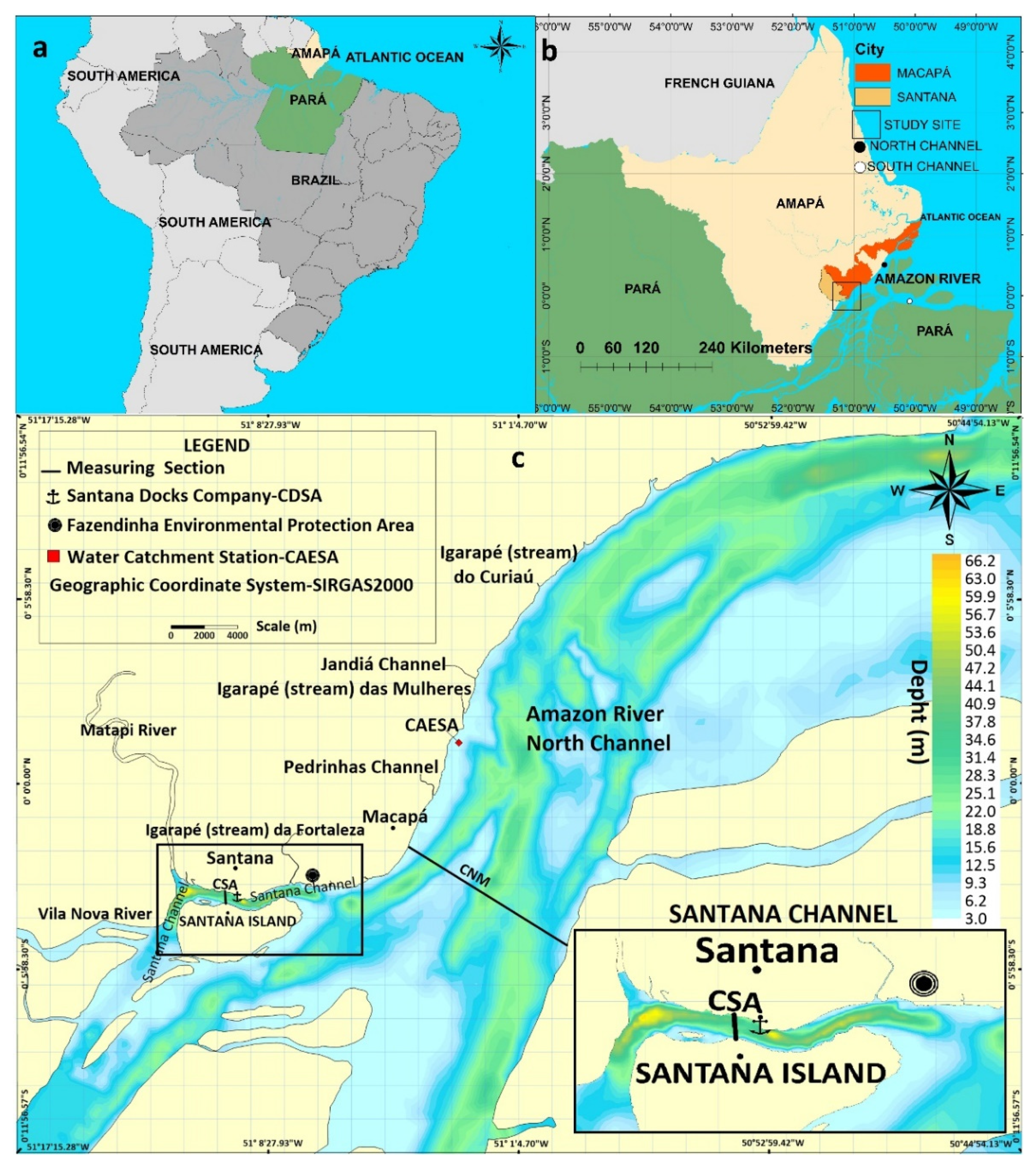
2.1. Characterizationof Study Site
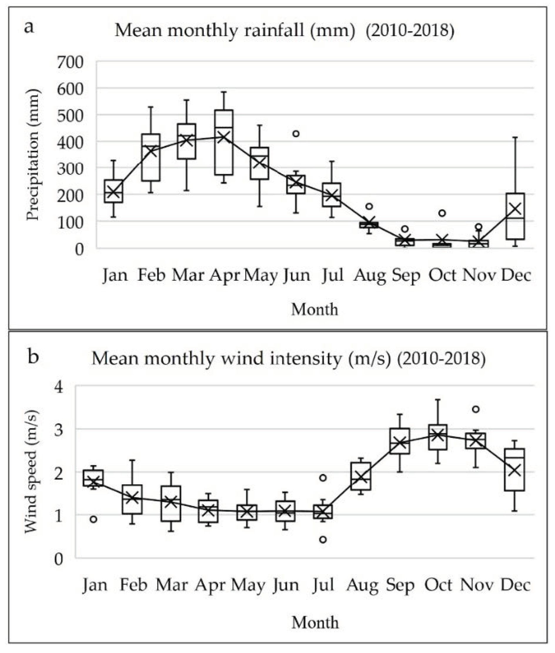
The research was carried out in a significant area of the North Amazon River Channel, which hosts the Santana Channel. Both channels are located in the coastal-estuarine zone of Amapá State/Brazil, Legal Amazon [2]. The selected estuarine stretch lies between Vila Nova River and Jandiá Channel (it is approximately 40 km long, and heads Southeast-Northwest Amapá’s estuarine coast). The CNM and CSA were the hydrodynamic and geographic references for the present study; they are located between Santana Island and Santana County (Figure 1).
The site where both channels are inserted in is 350 km long; it is flat, very low and unstable, as well as suffers strong influence of fluvial (North Channel of the Amazon River) and coastal (flood tide) processes that lead to erosion and deposition. These processes are responsible for the development of flooded plains at the mouth of the channel. There are numerous paleochannels in this stretch, which are evolutionary witness of a fluvial-lake plain. According to [46], the geomorphological types of lowland estuaries are relatively shallow and are rarely deeper than 30 m, with a high width/depth ratio and a cross-sectional area that increases the estuary below. Sometimes this growth is exponential and V-shaped.
This estuarine coastal zone is divided into three sectors: high, medium and low [2]. The high estuarine coastal sector is characterized as a stretch of Macapá Bay; the plain in this bay is often interrupted by tertiary formations (sediments from Barreiras Group) that look like cliffs. Abandoned meanders, residual lakes and “undertows” are observed in the coastal plain. The term ‘undertow’ is related to coastal wetlands, which consist of lagoons and lakes (influenced or not by the tide) exclusively seen in urban areas of Macapá and Santana counties, influenced or not by the tide, besides the presence of mangroves, in the edge of Macapá Bay [2].
This region also presents outstanding ecological-environmental importance because it is under constant anthropic stress caused by its proximity to Santana City and Macapá (the State capital). According to estimates from 2019 by the Brazilian Institute of Geography and Statistics (Instituto Brasileiro de Geografia e Estatistica-IBGE), these cities house 121,364 and 503,327 inhabitants, respectively; moreover, they are urban zones that present very low indices of basic sanitation and high urbanization-disorder degree. According to the 2019 sanitation ranking of the Trata Brazil Institute (Instituto TrataBrasil), Macapá City ranks 95 among the 100 biggest analyzed counties [41,42,43].
Santana County is the location of the Santana Docks Company (Companhia das Docas de Santana—CDSA), which is a strategic harbor for commodities’ dispatch (Manganese, wood, eucalyptus and cellulose) in Amapá State. This harbor constantly receives and dispatches cargo coming from, and going to, other Amazonian regions; therefore, it is a mandatory navigation route within North Amazon River Channel (Figure 1) [45].
Macapá and Santana counties are located 250 km away from North Atlantic Ocean. Only the purely fluvial behavior of the Amazon River is taken into consideration in this region [47]; in other words, it does not suffer with saline influence due to intrusion, but it keeps its hydrodynamic behavior due to typical estuarine tidal variations. The observations from experimental campaigns and data from CDSA’s tide station have shown that local tide in this region has energy enough to rise the water blade by approximately 3m and to twist the outflow direction in the channels.

2.2. Climatic Data

Due to the climatic characteristics of the study region, with high rainfall, high temperatures (never lower than 18 °C) and a very sharp dry season (August to November), the classification climate according to Köppen’s methodology is Am (Monsoon climate) [48]; in this region it is possible to split the climatic variation into two main periods: the Amazonian rainy period, which takes place in the first half of the year (from Jan–Aug), with higher intensity between March and May; and the lesser rainy Amazonian period (Sep–Dec), which is more intense in the second half of the year, between September and November [49,50,51].
Similar to rainfall, variations in wind intensity are seasonal. Wind velocity is lower in the rainiest period and the opposite is observed in the lesser rainy period (higher intensity). Meteorological data in the current study (rainfall and wind intensity) are shown in the graphs depicted in Figure 2a,b, whose historical series was based on an 8-year time interval (2010–2018). Data were collected at Macapá’s meteorological station (MACAPA-AP-OMM: 82098), which is located close to Fazendinha Environmental Protection Area. Data were provided by the Meteorological Database for Education and Research (Banco de Dados Meteorológicos para Ensino e Pesquisa-BDMEP) of the National Institute of Meteorology of Brazil (Instituto Nacional de Meteorologia-INMET).

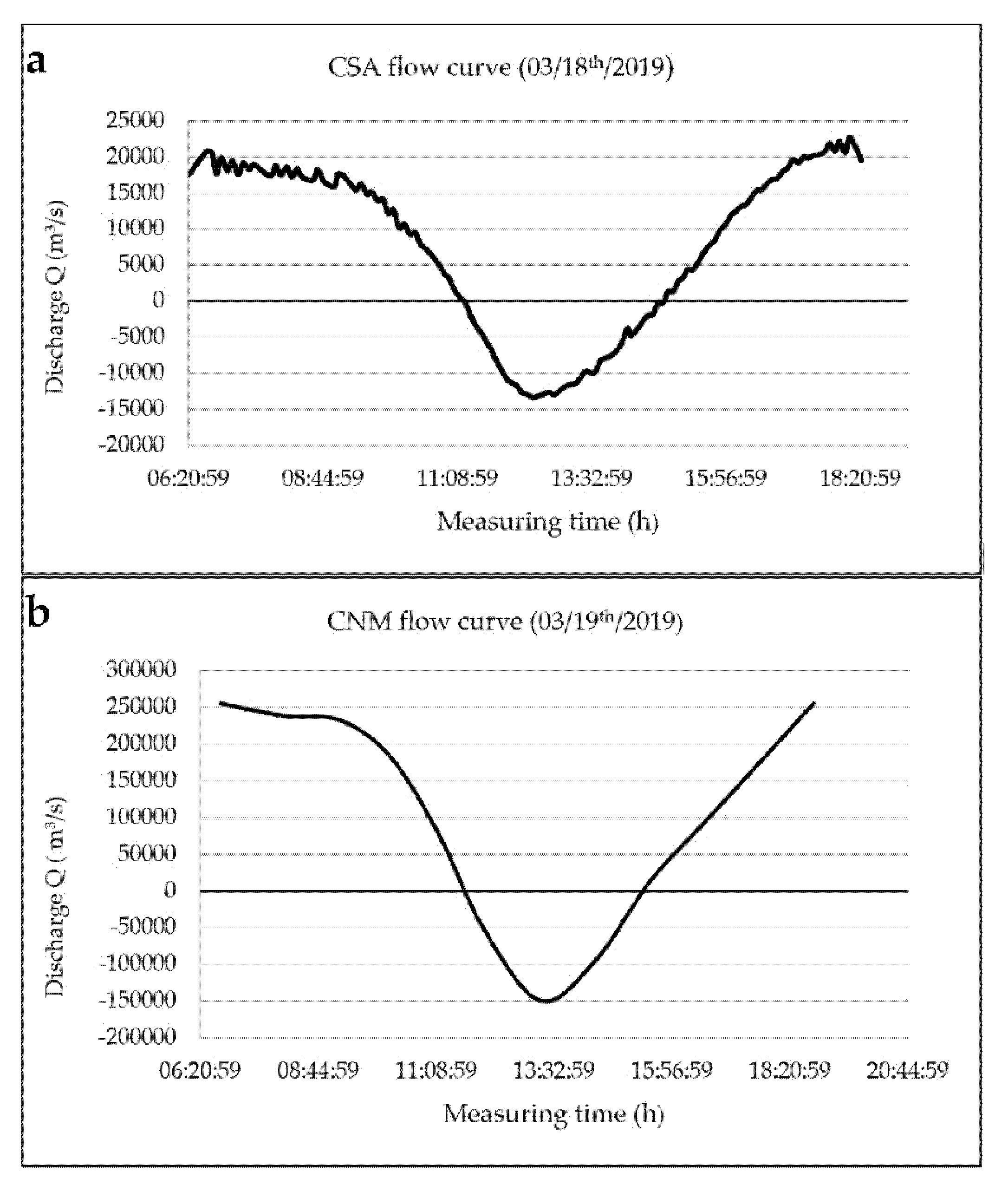
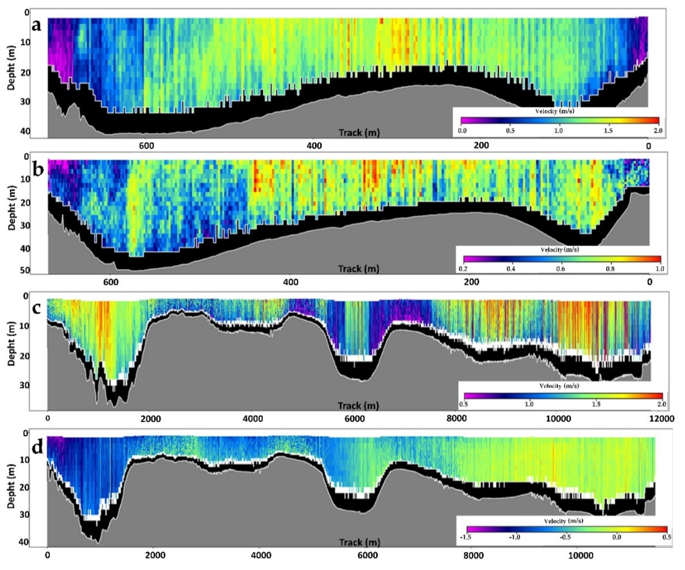
2.3. Experimental Campaign to Determine WaterDischarge Using ADCP: Santana-CSA Channel and North Amazon River Channel-CNM

The CSA and CNM channels were strategically selected to assess the natural outflow behavior of two large waterbodies affected by the same boundary conditions observed in opened channels; although their geometric and geomorphological features were different. The experimental campaigns were carried out in CSA (18 March 2019) and CNM of the Amazon River (19 March 2019). This was an essential stage, because there are no detailed data about water discharge in CSA to evidence a complete tidal cycle (12.5 h). Thus, unique experimental information necessary for model calibration and the simulation of hydrodynamic scenarios were herein generated. However, outflow measurements taken in CNM were added to a series of outflow data from similar studies previously conducted in this region [52] and Óbidos’ water station.
Both campaigns took approximately 13 h (tidal semi-daytime cycle) and were carried out through the Doppler acoustic method (Acoustic Doppler Current Profiler—ADCP) utilizing the model River Surveyor M9 of SonTek from Laboratory of Chemistry, Sanitation and Modeling Environmental Systems (LQSMSA/UNIFAP). The ADCP was installed at the side of a 22-m ship. Its transductors were immersed 1.0m down the water surface and connected to a notebook that was used to send commands and to control the data collection process and also GPS compass calibration in the analysis session.
The collection of data about flow in the CSA was carried out between the quadrature and syzygy periods, on the 18th of March 2019 from 6:00 am to 6:30 pm—this time interval covered a complete semi-daytime tidal cycle. In total, 133 crossings were performed in the cross-sectional section, whose mean extension was close to 650 m—each crossing took approximately 5 minutes (Figure 1). The referred estuarine stretch was chosen based on the following selection criteria: navigation safety; adequate depth; lack of sand or rock banks, or of Islands presenting outflow physical features adequate to reliable hydrodynamic measurements through ADCP.
The collection of data about flow in the CNM was conducted on the 19th of March 2019 from 6:45 am to 6:50 pm based on the same criteria applied to the CSA. The measurement process in the CNM only counted on 12 crossings through the cross-sectional section because the CNM is approximately 12 km wide (Figure 1); therefore, each crossing takes approximately 1 hour.

2.4. Hydrodynamic Simulation Process Development—Water Residence Time (Rt)

The program SisBaHiA was used to carried out the hydrodynamic simulations, the tidal prediction analyses and the seasonal Rt estimates (May, August and November) for the CSA and CNM. This software used the three-dimensional (3D) or the optimized 2DH (two-dimensional horizontal computational model vertically integrated) model of hydrodynamic circulation applied to natural waterbodies, as well as Eurelian and Lagrangian models (water residence time) applied to transportation phenomena [39]. However, due to the aims of the present study, the 2DH model (Equations (1)–(3)) were as used to represent the hydrodynamic behavior; the Lagrangian model (Equation (4)) was adopted to simulate Rt.
U t + U U U x + V U y = g ζ x g H 2 ρ o ρ r x + 1 H ρ o ( ( H τ ˆ x x ) x + ( H τ ˆ x y ) y ) + 1 H ρ o ( τ x S τ x B ) 1 H ρ o ( S x x x + S x y y + 2 Φ s e n θ V U H q
V t + U V U x + V V y = g ζ y g H 2 ρ o ρ r x + 1 H ρ o ( ( H τ ˆ x y ) x + ( H τ ˆ x y ) y ) + 1 H ρ o ( τ y S τ y B ) 1 H ρ o ( S y y y + S x y x 2 Φ s e n θ U V H q
ζ t + U H U x + V H y = q
Wherein, U ( in both equations) is defined as the velocity in axis x (m/s); V is the velocity in axis y (m/s); ζ represents the free surface elevation (m); H is the water-column depth (m); ρo is the mean water density (kg/m3); ρr is a reference water density (kg/m3); g is gravity acceleration (m/s2); τij is the turbulent stress tensor, and (i, j) represent the indexes in the horizontal (x; y) plane; τ i S and τ i B are the wind stress on the water surface and the bottom friction stress, respectively (kg/ms2); 2ΦsenθU and 2ΦθsenV represents the Coriolis accelerations, Φ is the angular velocity of earth rotation (rad/s); θ is the angle of latitude, and ∑q represent the flux balance of rainfall, infiltration, and evaporation; and Sij represent the radiation stresses effect [39,53].
The model considers the uncompressible outflow, such as that of shallow waters; i.e., density within a moving flow-control volume is considered constant. This definition is necessary to make it possible performing the numerical calculations for the current analysis.
Based on the traditional concept, Rt is calculated through the ratio between compartment volume (m³) and the residual water flow (m³/s) through the compartment. However, there is great spatial complexity and heterogeneity in the stretches of the natural channels, such as that in the present research, once the several flow conditions in the space, in a certain instant in time, as well as throughout time are predictably known. Thus, this heterogeneity is seen as a function of water residence time in the model; it can spatially vary due to flow conditions characteristic of different water hydrometeorological forcing throughout time [39].
Transporting constituents in the Lagrangian model was performed on the SisBaHiA, which are represented by a number of immaterial particles transported by currents counted through the hydrodynamic model. The position of any particle in the following instant (Pn+1) is determined by a second-order expansion in Taylor’s series based on the known previous position (Pn). The governing equation for particles tracking is expressed as (Equation (4)):
P n + 1 = P n + Δ t d P n d t + Δ t 2 2 ! d 2 P n d t 2 + O 3
In the model it is assumed that the velocity field promotes the transport of particles that corresponds to the velocities calculated by hydrodynamics. After calculating the position of the particle, the effects of the diffusive velocity field can be included, by means of random deviation from its position. This calculation of the random deviation is performed according to the spatial derivatives of the turbulent diffusivities [39].
In the SisBaHiA, two groups of boundary conditions are possible through closed boundary nodes for imposing water discharges values and open boundary nodes for free surface elevations values [54]. In the open boundary a water surface elevation series was imposed to represent the waves. In this context, the model was parameterized with the six main tidal components (M2, S2, N2, K1, O1 and M4), which were imposed in nodes of the mesh of the open boundary (Figure 3). In the closed boundary water discharged from the Amazon River was imposed (collected in Óbidos station and experimental data in CNM) and two of its main tributaries (Xingu and Tapajós rivers). In the lateral and bottom boundaries impermeable and no slip conditions were imposed. As the initial condition, constant values for elevation and velocity were used [52,53].
Initial contour data for the simulations were collected and inserted in the model (flow, tidal range, wind velocity intensity and direction; bathymetry, roughness, and rainfall). Flow-related data were inserted in it based on the measurement campaign carried out in the CSA and CNM between18–19 March 2019 and on other similar research conducted in the region available in the literature [52,55]. Moreover, ANA data were collected in Óbidos’ station (code 00155001). Data about rainfall, wind direction and intensity were collected in Macapá’s meteorological station, which were provided bytheMeteorological Database for Education and Research(Banco de Dados Meteorológicos para Ensino e Pesquisa—BDMEP)of the National Institute of Meteorology of Brazil(Instituto Nacional de Meteorologia—INMET).

2.4.1. Computational Mesh

Computer domain mesh covers an area of approximately 3 × 10⁷ km2. In total, 2,238 elements were distributed in this area, thus totaling 10,627 nodes. This region is the biggest computer domain, it is located West, between Araguari River (AP) and South in Almeirim (PA). It was delimited to include the CNA and CSA stretches in the present research. So, the hydrodynamic simulation and Rt outputs were analyzed (Figure 3).
Bathymetric data (depth) were collected from the Brazilian Nautical Charts of the Brazilian Navy (Diretoria de Hidrografia da Marinha (DHN)/Centro de Hidrografia da Marinha (CHM)) [56]. These data were inserted in the computer domain of the study site, which counted on approximately 17 thousand points distributed to define the depth profile between the Araguari river and Almerim city (Figure 3). After these data were inserted in the bathymetric model, they were “leveled” to the same altitude to correct the tidal fluctuation behavior of each sub-region of the computational domain. The corrected levels were subsequently subjected to the Kriging-type interpolation process in the Surfer software, version 9 (Golden Software, LCC). The 30/30 spacing was adopted to find the most accurate interpolated depths possible for the model. This same method was applied to the spatial distribution of rough attributes in the computer domain shown in Figure 3 [57].
Tide generation in the boundary of the model’s spatial domain is an important phase of the hydrodynamic model’s parametrization process, which used the most relevant harmonic constant for the study site (M2, S2, N2, K1, O1, and M4). These constants were selected due to their relative influence on tidal wave generation in the mouth of the Amazon River; mainly in harmonic M2, which represented up to 70% of the tidal physical behavior influence on the region [58,59,60].

2.4.2. Model Calibration and Evaluation Process for the Water Residence Time Analysis (Rt)

The strategy used to calibrate the hydrodynamic model was to match the simulated results and field measurements as closely as possible within acceptable ranges by adjusting the parameters requiring calibration [61]. There is in the specialized literature a variety of analyses able to be applied in calibration processes [62,63].
For evaluating the model robustness, we have considered a comparison between observed and modeled time series of water level-height of stations within the computational domain. In this understanding, [63] reported that a satisfactory comparison with field data serves as verification for the model properly simulates all the forcing combined.
As before mentioned, in the calibration, we performed the model with six of the main harmonic constituents (here, M2, S2, N2, K1, O1, and M4) at the open boundary. The value of the constituents was imposed in the nodes of the open boundary using adjustment of coefficients (in amplitude and phase) for each harmonic constituent. A similar methodology was used in [35,63,64].
The harmonic analysis was performed on the time series of the model simulated for water surface elevation. In Figure 6, for example, the series of predicted and computed water levels for the analyzed period were compared. The predicted and modeled tidal data show the correct and satisfactory representation of results explained by the coefficients of correlation set between the observed and simulated results (r2 > 75%) (Table 1 and Table 2).
The strong influence of bottom roughness on the wave propagation in the CSA and CNM channels was not detected, due to the large variability of the depth. Furthermore, a correction of the bathymetry located in the open boundary was carried out to obtain the best reproduction of the data of currents measured in the field. The numerical parameter used in the eddy viscosity model was 0.25, and the width of the Gaussian filter for direction x and y was of 0.5 (parameters in the momentum equations (Equations (1) and (2)). The SisBaHiA adopted turbulence model consists of filtering techniques in a way similar that the large-eddy simulations approach of Gaussian filtering functions.
However, tide elevation data from 2016 collected in CDSA were used in the analysis, once that is done the maintenance of the quality and consistency of numerical outputs are optimized. Such analysis aimed at reproducing the same tidal harmonic components in the study site to be projected on another period (2019) at the lowest error possible. The series was considered consistent with the tidal projections set for 2017; 2018 after the procedure and the analysis of statistical results was performed in the prediction stage. Similarly, it was also possible comparing modeled data from the referred periods to predictions made to 2019. This procedure was done by observing their respective statistical significance.

2.5. Statistical Analysis

Statistical analysis was used as a security tool to assess the results of tidal predictions generated in SisBaHiA, by comparing them to tidal behavior recorded in March and November 2017 and in May and August 2018. The statistical analysis applied to the modeled results from May, August and November of 2019 was compared to tidal predictions for 2019. The flow behavior in the tidal cycles experimentally observed in the field was checked. This procedure was followed by new comparisons to results simulated by the model for March 2019.
Classical tests were adopted to quantify the efficiency of mathematical models: Nash–Sutcliffe Efficiency (NSE) (Equation (5)), Person’s correlation, r2 and Index of Agreement (d) (Equation (6)). These tests were selected given their different practical applications in hydrodynamic modeling for water studies, i.e., to test the accuracy and capacity of the models to represent the physical reality [65,66,67,68].
E NS = 1 i = 1 n ( O i P i ) 2 i = 1 n ( O i O ¯ ) 2
d = 1 | P O | 2 ( | P O ¯ | + | O O ¯ | ) 2
Wherein, Oi and O represent the observed tide elevations; Pi and P values represent values predicted by the model. Model efficiency results can range between 1 and −∞ in Equation (4) (Nash–Sutcliffe’s Efficiency), wherein 1 indicates the model that perfectly represents the observed data. Values higher than 0.75 indicate the model capable of well representing what was experimentally observed [69].
Similar to the NSE efficiency test, the Index of Agreement test (d) compares data generated by the model (P) to the observed data (O): if d = 1, the model is considered perfectly coherent; if d = 0, the model shows lack of ability to represent the reality of the observed data set. The minimal acceptable value for “d” would be 0.75.

3. Results

3.1. Overall Results Recorded for the Experimental Data: Santana and North-Macapá Channels

Results of field campaigns carried out in Santana (CSA) and North-Macapá (CNM) channels are represented by semidiurnal flow curves (Figure 4a,b). The maximum ebb and flood outflow values recorded for CSA in the field were of 22,729 m3/s and −13,381 m3/s, respectively. Once the climatic event that took place when the measurements were taken, some data captured by ADCP in the CNM were not properly continuously stored. Thus, it was necessary to interpolate the last measurement series. However, it was possible observing that the maximal outflow value was at the order of 254,944 m3/s; this value was −149,653 m3/s at flood (Figure 4b).
Figure 4a,b suggests that the behavior of the CSA and CNM flow curves is directly influenced by the tide coming from the Atlantic Ocean. The reversion period (flood) was significantly shorter in both channels between 3 h and 20 minutes and 3 h and 40 minutes than in the ebb outflow period, between 8 h and 20 minutes and 8 h and 40 minutes.
The two measurements selected for each one of the channels show details of the punctual velocity variation behavior and of the bathymetric profile in the measurement section conducted in the CSA and CNM, taking into account the ebb outflow and flood peaks. Data were extracted from the River Surveyor software and depicted in Figure 5a,b (CSA) and Figure 5c,d (CNM).
The greatest velocity intensities in CSA (Figure 5a,b) were closer to the center of the channel than to its edges (it was highlighted by the contrast between light and dark colors) in the section where measurements were taken with ADPC during the ebb outflow and flood periods. Velocity in some points during CSA’s tide flow (22,729 m3/s) can reach 2 m/s, whereas velocity range was limited to the maximal value of −1 m/s during the flow (−13,381m3/s).
Velocity significantly changed in CNM in comparison to CSA. It is possible observing that velocities were higher in the sides of the river (by taking into account the natural ebb outflow direction) than in the center of the channel—it presented maximal punctual values up to 2 m/s (ebb outflow) and 1.5 m/s (flood). It is important pointing out the significant spatial asymmetry in outflow rates during water discharge measurements taken in CNM. Such asymmetry has caused significant velocity and flow variation throughout the sub-sections during the experimental measures.
The bathymetric profile of the study site showed that depth variations throughout the CNM’s measurement stretch highlighted at least three “sub-channels” or “secondary channels” (Figure 5c,d). Depth in the first sub-channel (from the left to the right side of the channel) reached ≈ 29–35 m, whereas the central part of the channel had ≈ 20 m and the right side of it could reach 25 m. However, by analyzing data collected through measurements taken with ADCP, it was possible finding depths up to ≈ 38 m. However, CSA showed two sub-channels and smaller variations in the depth than in CNM, because its measurement section was smaller.

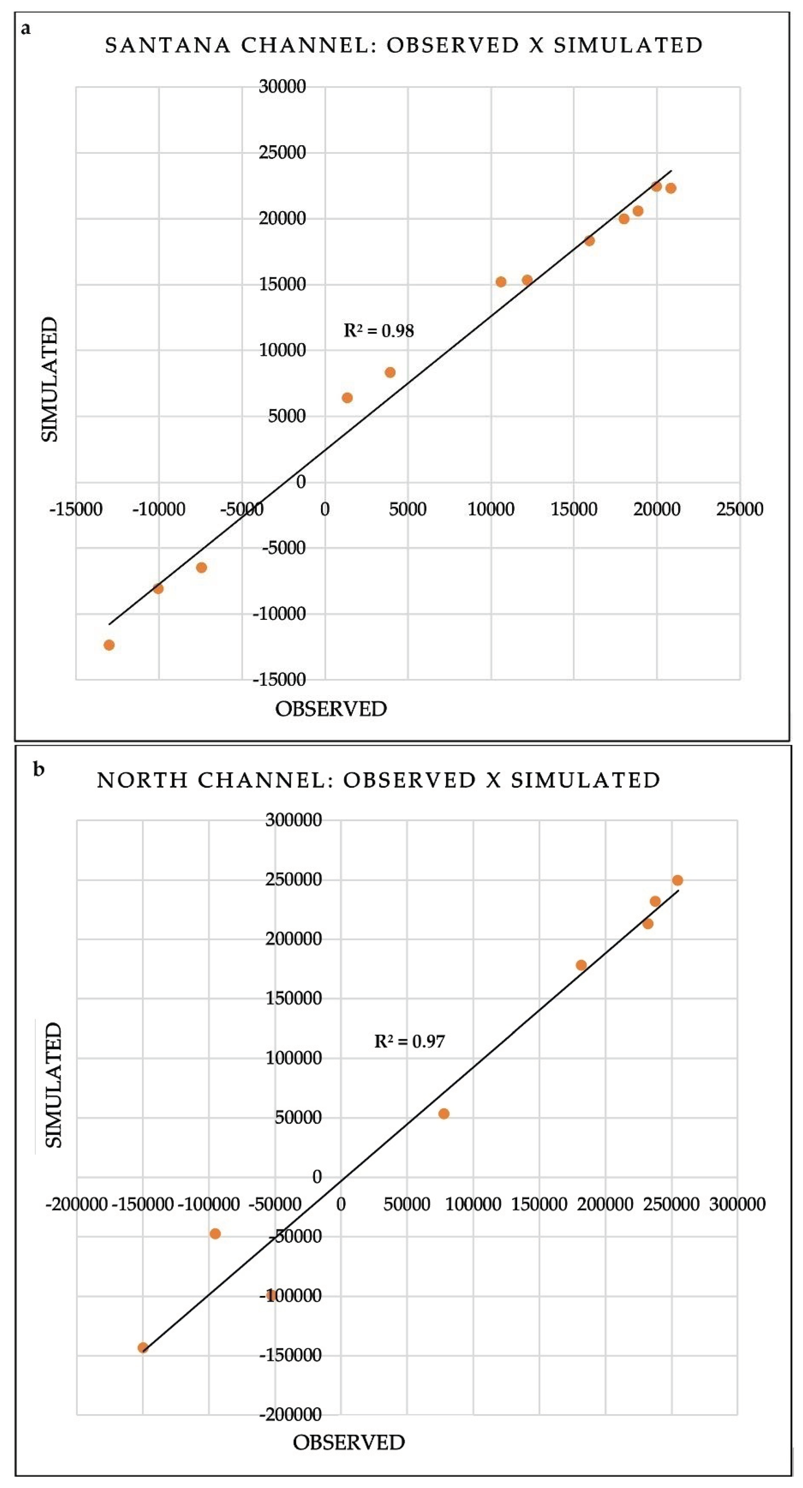
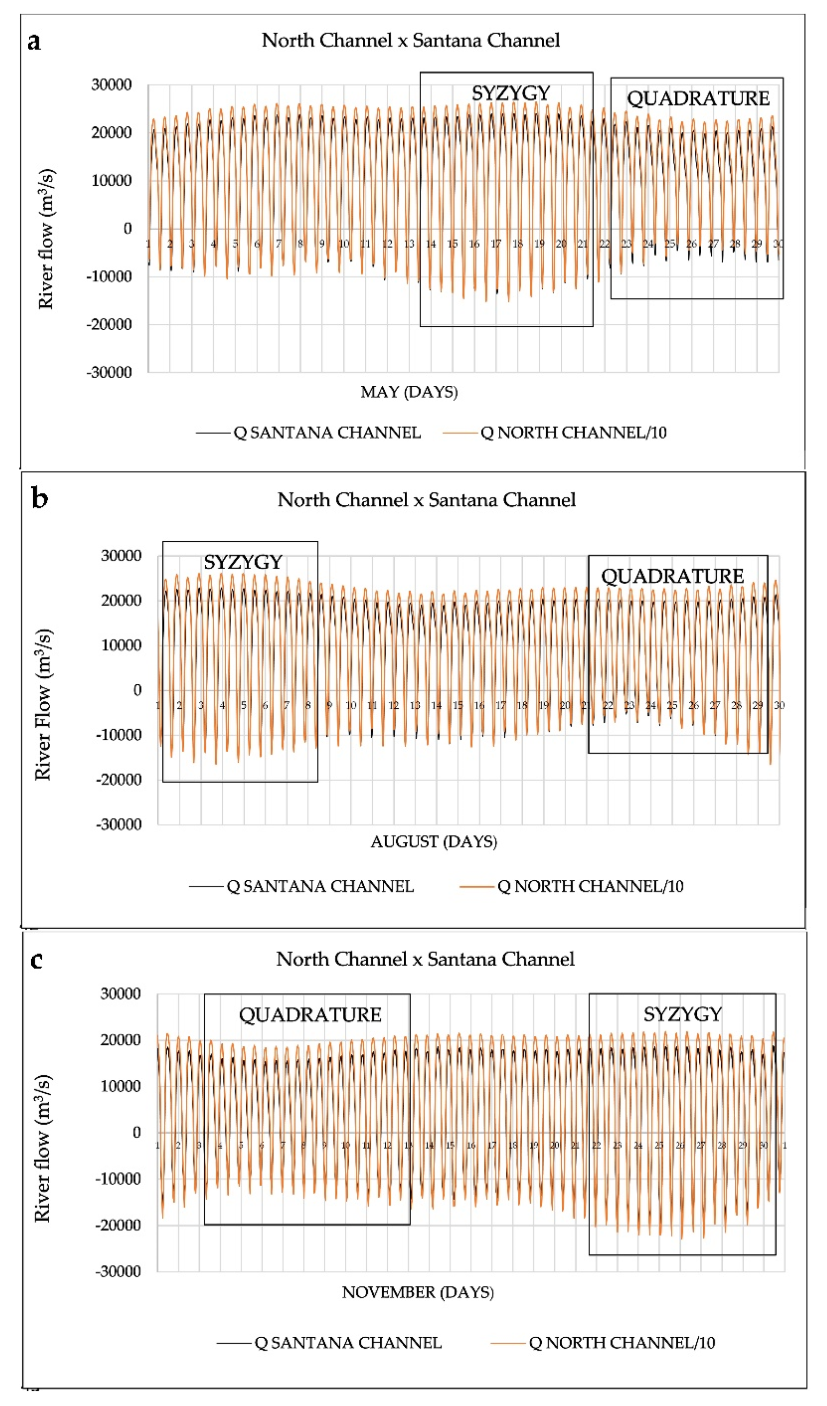
3.2. Statistical Analysis and Model’s Response to Tidal Predictions

The hydrodynamic model was calibrated with the aid of harmonic constants generated by the analysis of data from the CDSA station in 2016. This stage is extremely dependent on monitored data from the station in charge of measuring tide level in Santana. Comparisons between tidal output data predicted by the model—compared to data provided by the CDSA tide station—were carried out to assess the consistency of prediction data generated in SisBaHiA for 2019. This process was applied in March and November 2017, and in May and October 2018.
Results were forced to reference level (zero); the graphic comparison between predicted and observed tidal variations in the CDSA tide station are presented in Figure 6a–d (orange curves point out the model’s prediction and blue dots indicate observational data of the same period).
Based on the predicted and observed results shown in the graphs (Figure 6a,b) and in Table 1, it is possible observing that the model satisfactorily predicted the behavior of CDSA station’s tidal phases for the specified periods (2017/2018, respectively).
Table 1 shows that tide behaviors predicted by the model in 2017 and 2018 are quite satisfactory and all statistical tests recorded values higher than 0.95. Thus, the statistical analyses allowed considering that these values are good enough to be the reference in comparison to other modeled results (tidal predictions) recorded for March, May, August and November 2019. These results are shown in Table 2.
As shown in Table 2, values recorded for all applied statistical methods also presented values higher than 0.95; therefore, the comparison between simulated data and the model’s predictions in SisBaHiA well represent the hydrodynamic behavior of the study site—it can also be safely applied to calculate Rt.

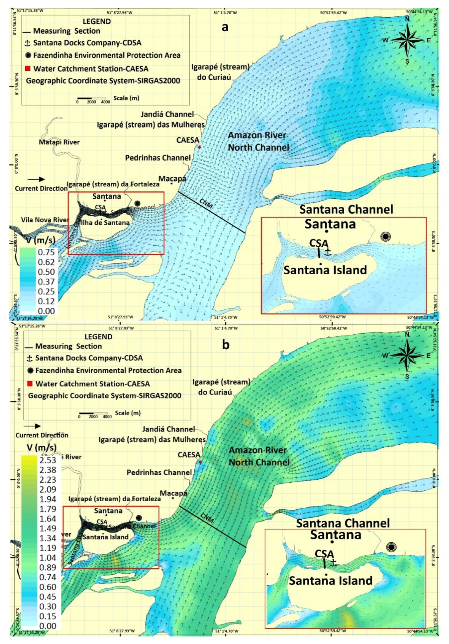
3.3. Hydrodynamic Behavior Analysis: Experimental (ADCP) and Simulated (SiBaHiA)

The present topic concerns the analysis of data simulated and compared to flow data (Figure 7a,b) measured in CSA and CNM (Table 2 and Table 3). Data generated in SisBaHiA produced full hours values (07:00; 08:00, etc.), whereas data measured in the field were recorded in fractioned hours (07:22; 08:35, etc.). Thus, a correction of the real hour approximation for the comparisons to the simulated hours was applied.
Figure 7a,b shows that the adjustment of r2 values to flow were higher than 0.95 in both channels. Moreover, the statistical analysis of tidal variation between 18 March and 19 March 2019 predictions carried out in SisBaHiA have also indicated values higher than 0.9 in the other statistical parameters: Person’s correlation, “d” and NSE.
Table 3 and Table 4 describe ebb and flood flows and velocity values in comparison to values simulated and measured in the field (in Santana and North-Macapá channels) by taking into consideration the semidiurnal cycle.
Relative errors between flows observed through ADCP measurements hada straight reflex on velocity values recorded in the field. However, as shown in Figure 5a, the greatest velocity magnitudes are observed in the center of the channel, whereas the smallest ones were observed in the sides of it. This behavior was expected and captured by the hydrodynamic model. The comparison between these values in CNM was carried out based on the same procedures adopted for CSA; however, the need for adjustments was lower because measurements taken in CNM took place within a longer time interval. Velocity and flow result analyses applied to data collected through the model or the ADPC measurements are shown in Table 4.
Figure 8a,b shows the CNM and CSA velocity behavior in the field during high-tide and low-tide periods on the 18th of March, 2019. Velocity’s in the low tides tend to be higher than in the high tides.
Figure 9a–c shows the ebb flow and flood flow behavior during the quadrature and syzygy periods in May (rainy period), August (transition period) and November (lesser rainy period) 2019. Table 5 presents the maximum values of ebb flow and flood flow rate observed in the relate simulated months.

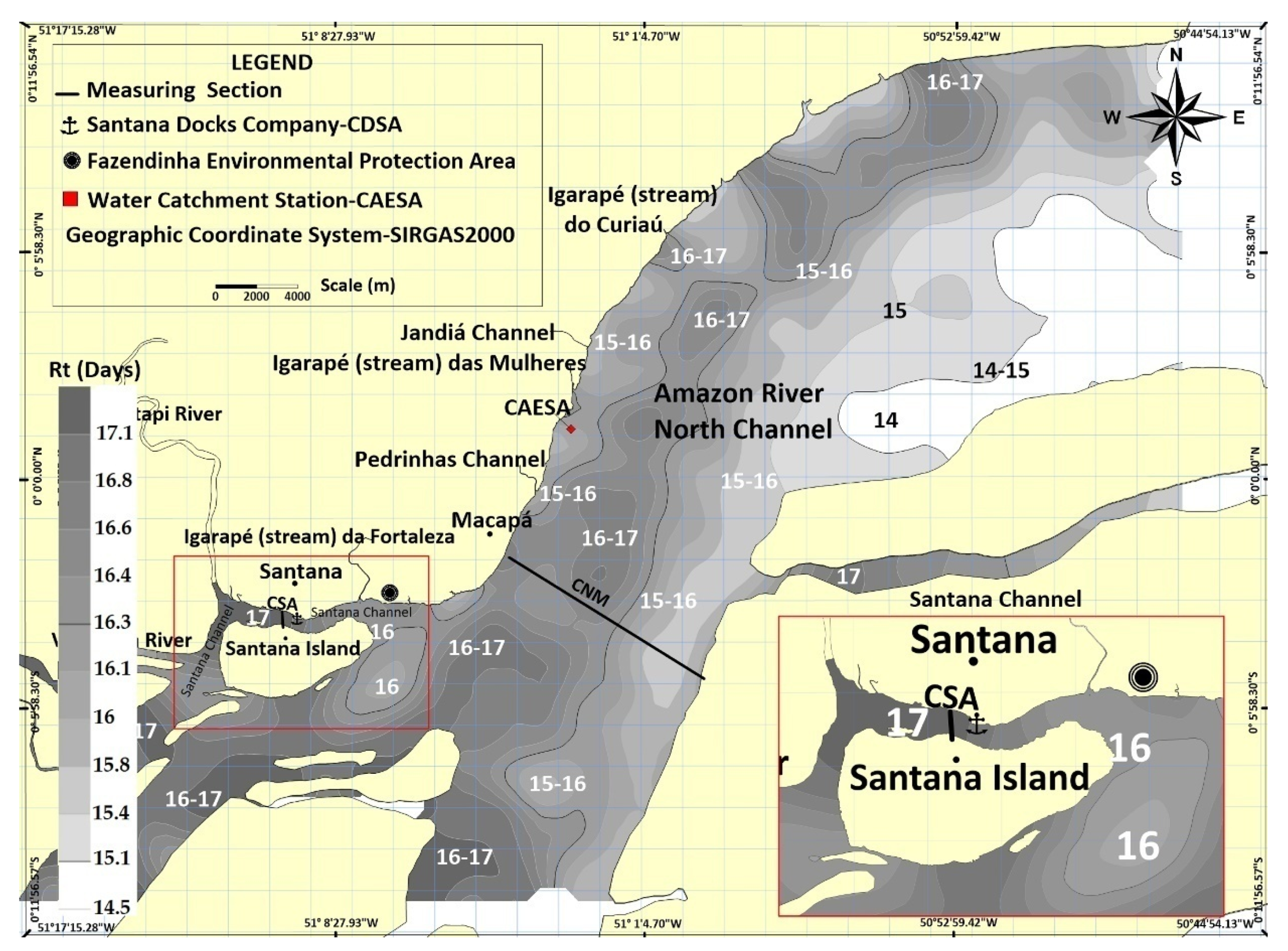
3.4. Water Residence Time (Rt) Simulated with the SisBaHia

Rt average in CNM recorded in May 2019 was approximately 16 days long (Figure 10); it changed within confidence interval ranging from 14.5 to 17 days. The analysis section was didactically divided into three “sub-channels” throughout the experimental and simulated measurement sections, which showed the likelihood of the right margin of the channelto record the shortest residence time (between 14 and 16 days) in comparison to the center of the channel (sub-channel of the medium). The center of the channel tended to record values higher than 16 days. Values in CSA also stayed higher than 16 days, and this outcome indicates a lower water renovation rate in this stretch. The mean flow value was observed in the period facing the highest rainfall in comparison to August (transition) and November (dry period) (Figure 2a). On the other hand, wind velocity intensity in this period was lower than in August and November (Figure 2b).
August was the transition period between the rainy (May) and the lesser rainy periods (November) in the study site. Figure 11 shows that August showed a small Rt increase from 14.6 to 17.7 days. However, despite the little variation in Rt between May and August, the mean ebb flow in August was 110,113 m3/s (14.7 % lower than the average recorded in May) in CNM and 8745 m3/s (19.2% lower than in May) in CSA. Such reduction resulted from the natural seasonal rainfall reduction typical of the Amazon basin (Figure 2a), which, consequently, diminished the ebb flow and, indirectly, increased Rt.
The highest Rt in May was concentrated in CSA and along the left side of CNM; its variation was close to 8 days. Furthermore, the central region and the right side of CNM presented relatively lower Rt values ranging from 15 to 16 days.
November is the dry period in lower Amazon River region, when one can observe the lowest monthly rainfall means (Figure 2a). But it is also the month recording the highest wind intensity (Figure 2b). The hydrodynamic model responded with mean ebb flow of ≈ 63,829 m3/s in CNM and of ≈ 4823 m3/s in CSA in this period. Thus, CNM and CSA values were ≈ 55% lower than in May; consequently, November presented even higher Rt values, as expected. So, the Rt values ranged from 15.5 to 22.4 days (Figure 12).

4. Discussions

Results of statistical comparisons among the observed, predicted and simulated data referring to water level variations in the CDSA station in May, August and November 2019 were excellent (Table 1 and Table 2). These results allowed concluding that the simulated water mass exchange in the study site was coherent with a plausible behavioral pattern. They presented approximately the same order of magnitude when they were compared to similar studies about the application of modeling processes in estuarine systems under tidal influence [64,66,67,68,69,70].
Results in the current study have also shown that the geomorphological features of the channels (variation and evenness in the channels’ depth and width) have caused asymmetries in velocity and in flow distribution either in CNM or CSA, as also observed in the field. However, these asymmetries were experimentally more perceptible during the longer crossings in CNM, when it was necessary almost one hour to cross the cross-sectional section of the natural outflow, as well as during the significant spatial and time variations (which seemed to be non-linear) in outflow hydrodynamic features, namely: change in tidal pattern (ebb-flood) and spatial changes in velocity direction along astretch and during the tidal cycle. This outcome suggests the clear secondary currents and circulations in the longitudinal and lateral directions of the outflow.
This typical behavior was also observed by [22] in Araguari River estuary, close to the mouth of the Amazon River. Another important result was also observed in the present study; it indicated similar behavior, namely: tide influence observed by [6] in Yangtze River, China, where tidal intensity changed the water flow patterns in the estuaries and produced bidirectional currents, as experimentally observed in the estuary of the Amazon River (Figure 9a–c) and in the model’s results (Figure 8a,b). Thus, based on the current results, when the experimental CSA and CNM flow curves were compared to similar behaviors described in other studies, it was possible stating that the numerical simulations well-represented the mean natural hydrodynamic behaviors (Figure 7a,b).
Regarding the water discharge measurements experimentally observed in CNM [50], it was possible seeing that ebb values have the same magnitude order, or order close to 176,681 m3/s, and 134,102 m3/s in the flood period at the lesser rainy period (October). On the other hand, this behavior was 255,625 m3/s in the ebb flow and −170,808 m3/s in the flood period at the rainiest period (March), respectively.
Thus, similar to the flow observed in CNM, it was also possible making a good adjustment between simulated water discharge values and values measured in the field (Figure 7a) in CSA. Similar behavior was observed in November (dry season) by [55], when the referred author recorded an experimental flow value of ≈ 18,385 m3/s in the ebb period and of ≈ −16,360 m3/s at the flood period. On the other hand, although simulations have presented tide value variations and water discharge close to the observed experimental data, current velocity has shown a trend to values higher than the experimental ones—indicated by ADCP in the field (CNM and CSA). Estimates have shown that such differences resulted from differences in the bathymetric features inserted in the model (based on navigation charts by the Brazilian Navy). In other words, the bathymetric methodology used by the Brazilian Navy to generate navigation charts used in the model can lead to different results in the assessment of CNM and CSA made through ADCP due to the interpolation process.
However, based on the chart of sea currents generated by the Brazilian Navy for this region, it is important to highlight that velocity variations at low and high tides were closer to the simulated results (Figure 8a,b) [71]. Figure 8a shows the slack tide behavior observed at high tide, when one can see that the magnitude of the current is smaller—values were close to zero; whereas, the currents were more intense at low tide, reaching values higher than 2 m/s.
Current behavior, tide elevation and water discharge results (May, August and November) of simulations ran in the model showed the bases for Rt studies and simulation in the study site. As expected, and observed in similar studies in the literature, Rt is a physical parameter directly dependent on, and sensitive to, the physical features of waterbodies and of their seasonal variations. Therefore, it has been used as important primary indicator in studies related to the quality of the water [25,26,27,28,72,73,74,75,76,77,78].
Rt values found in the simulations set for CSA and CNM have presented significant seasonal and spatial changes, which ranged at values a little higher than 14 days and a little lower than 25 days. Rt in CNM, for example, ranged between 14 days ≤ Rt ≤ 22 days, and showed different behavior and spatial variations throughout the computer domain (Figure 10, Figure 11 and Figure 12).
In this case, it was possible assuming that the spatial variation in Rt happened due to the bathymetric differences that have influenced the variation in water mass volume (distribution), which was unevenly distributed in the spatial domain. These differences were observed in ADCP data, as well as in navigation charts inserted in the model (Figure 1); they evidenced “sub-channels” in the CNM monitoring sections, such as the sub-channels located at the left and right sides of CNM, which have presented different water volume.
As previously mentioned, Rt spatial variations can be associated with biogeochemical processes that depend on seasonal variations in the tidal cycle of the Amazonian estuary [12,13,15,23], on complex interactions between channels’ geomorphology and roughness and, mainly, on interactions and exchanges of different water masses in different simulated control volumes and in the computer domain volumes [79].
Physical gradients controlling the water masses entering, leaving or accumulating in each unit volume are interesting highlights in these interactions -they show the dependence between currents and tidal phases (Figure 10, Figure 11 and Figure 12). These tidal phases get more intense as the flood period and the maximal annual water pulse approach [10,22,23]. On the other hand, some of these factors have not been taken into account in the water balance of great water bodies, such as the estuary of the Amazon River, once there is a series of the experimental barriers and high complexity of hydrodynamic modeling processes. However, actually, as these hydrodynamic parameters are inserted in the analysis, they add more complexity to the numerical analyses, mainly, to Rt estimates.
Rt values in the rainy (May 2019) and transition (August 2019) periods in CSA and Santana Island surroundings (Figure 10) remained close to 17 days (Figure 10, Figure 11 and Figure 12). This value was higher than 20 days in the lesser rainy period (November 2019); i.e., the volume of exchangeable water in the rainy months tends to be effectively higher, and the water mass is apparently more distributed in the spatial domain. The greater likelihood of maintaining the concentration of passive agents in the water in time (nutrients, chlorophyll, pollutant, among others) is an important ecological consequence of it [74].
It is possible seeing lower Rt values by comparing the hydrodynamic behavior of CNM and CSA to other lentic systems (great lakes and slow rivers). This outcome results from the fact that, despite its huge water volumes, this ecosystem is highly capable of renewing its water masses due to its corresponding and proportion flows. The high river flow in CNM, for instance, presents an average higher than 1.0 × 10⁵m3/s, velocity’s higher than 0.5 m/s and maximal velocity up to 2.0 m/s in this stretch of the Amazon River. These features point towards a lower likelihood of passive or cumulative agents’ permanence in the outflow (nutrients, or less pollutants); it would also allow greater ability to avoid eutrophication processes (algae blooming), even in case of severe environmental degradation [75,80,81]. In other words, the longer the water remains in the control volume, the greater the likelihood of passive flow agents remaining in the body of water. However, depending on the passive agent in the flow, this characteristic can be positive, for example, nutrients to feed the aquatic biota, or negative, to disperse pollutants [18,22,23,35,43,44,45].
Water renovation processes in lentic eutrophic estuaries can last weeks or months; in these cases, the water masses would present a higher likelihood to consume more dissolved oxygen [76]. However, such high oxygen consumption has not been observed in similar studies carried out in Macapá and Santana regions [43,82]. Thus, a more detailed local analysis could suggest the occurrence of two processes unfavorable to dissolved oxygen depletion, both linked to Rt: (a) pollutant load is not significant in comparison to the exchange capacity or to water dilution volume, which has almost no significant influence on degradation levels; (b) oxygen consumption rates would be much lower than self-depuration rates due to atmospheric reaeration (turbulence), which is bond to Rt. There is a third assumption, according to which, water biogeochemical features (the presence of high or low organic load in the water column) could favor certain kinetic processes (HZ, for example) and avoid more critical dissolved-oxygen consumption (sediment, for example).
However, Rt determination has been frequently focused on estuarine systems located close to the river mouth to assess saline plume and pollutant dynamics. This parameter is little assessed in strictly fluvial systems (or only in the presence of drinking water) [83]. For instance, a study carried out in an estuarine system of Santos Basin (SP), showed the presence of saline plume. The referred author simulated Rt behavior [84] and estimated a value close to 30 days; therefore, when Rt value was compared to results in the present research, such value was relatively close to that of the estuarine system in Santos Basin at the dry period (November); of the period presenting lower rainfall and of the period when there was greater oceanic tide influence over upstream Amazonian estuary. In other words, saltwater is potentially more influential in the estuary at this period [10].
But, even by taking into account that Rt values relatively lower in CNM and CSA, in comparison to eutrophic estuaries and lentic bodies addressed in the literature, this value seems to be even higher than the expected for waterbodies presenting high river discharge. Assumingly, this finding regards the fact that water flow direction reverse in large dimension rivers tends to induce greater water mass permanence in the control volume than similar rivers, at smaller scale—without tidal influence [79].
Therefore, understanding Rt spatial and seasonal in lower Amazon River helps improving knowledge about the physical mechanisms of these aquatic ecosystems, being essential for the analysis about the exchange dynamics applied to nutrients and particulate, and even dissolved materials in the Hyporheic Zones (HZ) (C, N, P). The HZ zones are directly affected by variations in the physical features of the water quality, which has straight control over water reactions and biogeochemistry [32,33,34,85,86,87,88]. Although the literature presents the relevance of Rt and hydrodynamics for many waterbodies by highlighting their roles in HZs and the biogeochemical cycles of aquatic ecosystems, there are considerable gaps in knowledge about how these factors vary in the estuary of the Amazon River.
These gaps have been mentioned in other approaches concerning the Amazon River, the atmosphere and the Atlantic Ocean [10,11,22,23]. Because Rt depends on annual and seasonal water pulse and shows variations in the semidiurnal tides, it becomes even more relevant to assess how Rt influences the behavior of passive agents in the outflow, in other processes in water masses and, consequently, in the quality of these water masses in these Amazonian estuarine ecosystems [23].
Although the present contribution helps better understanding the mechanisms involved in Rt quantification, new scientific efforts must be made to provide information about the functioning of these aquatic ecosystems in the Amazonian estuarine complex. It is still necessary to deepen the subject, asthe ecological relevance of its aquatic biodiversity richness are still potentially unknown [18], because studies carried out in HZs in lower Amazon River are very rare, but these processes still continue and are naturally dependent on Rt.
Despite the experimental and numerical barriers found in the present research, it is essential taking the first step towards assessing how Rt influences biogeochemical processes dependent on its own interactions in tropical aquatic ecosystems. In this case, it is essential understanding Rt’s variations in space and time based on the complex characteristics of these channels [20,21,22,23,35].
Thus, the physical basis addressed in the present study about Rt, although yet little explored in the overall literature, shows its potential to future complex analyses on the hydrodynamics of the Lower Amazon River [13,47,89]. This is a necessary approach for coastal studies carried out in this region. To the best of our knowledge, studies presenting such in-depth analysis about Rt in the estuary of the Amazon River were never conducted before.

5. Conclusions

The hydrodynamic scenarios generated with SisBaHiA have shown that hydrologic and spatial variations have significant influence on river water renovation rates (Rt). Below, find the most relevant conclusions observed in the current study:
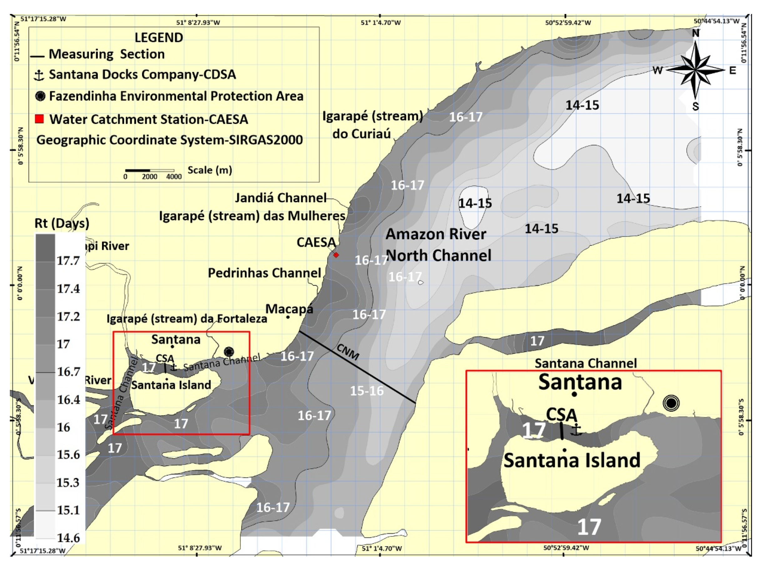
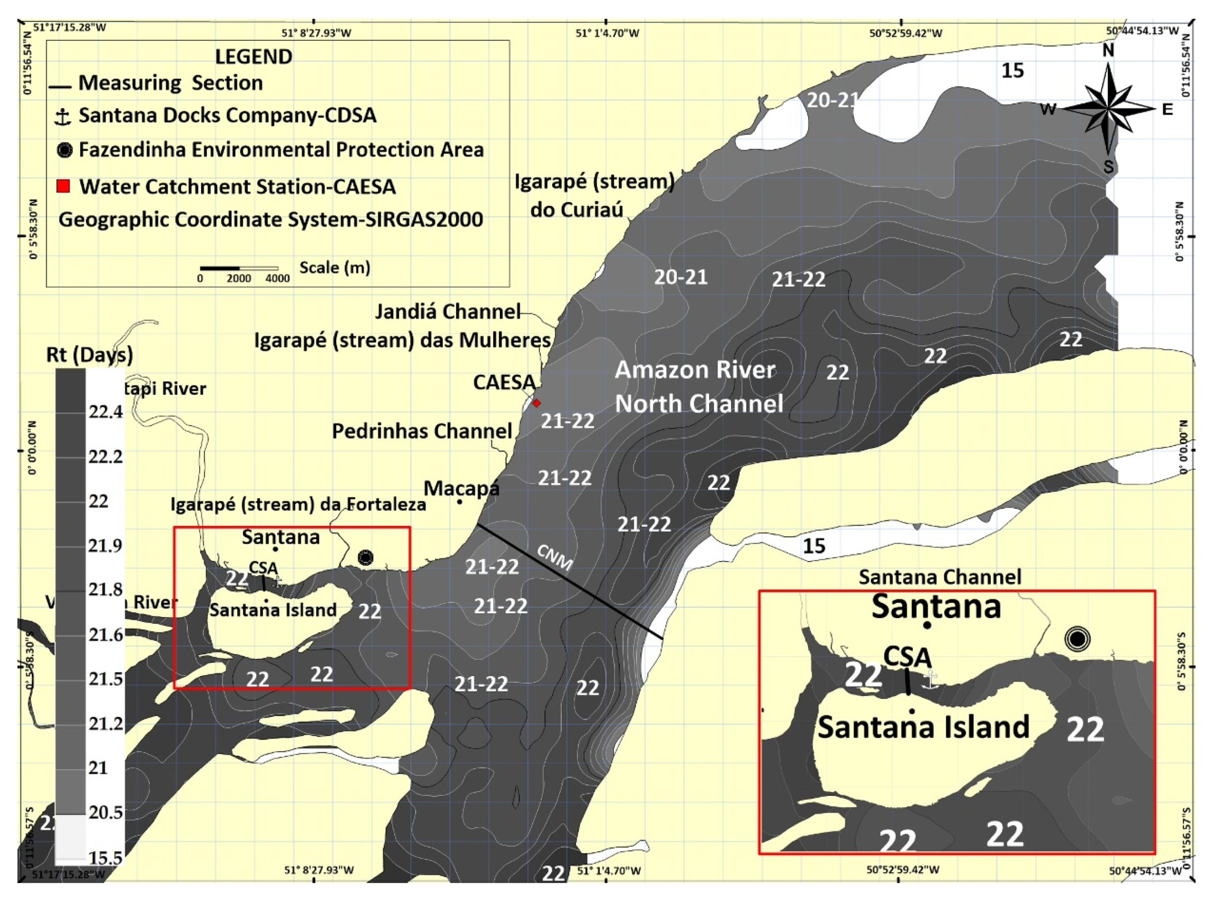
  • The simulated scenarios have confirmed the hypothesis that Rt presents values within a relatively restrict interval in the assessed period, between 14 days ≤ Rt ≤ 22 days. Therefore, time variations in water level predicted in the hydrodynamic model of the SisBaHiA software were adequate and satisfactorily calibrated. So, it was possible estimating variations in the Rt parameter in at least three seasonal water scenarios—Rt values were higher at the rainy period.
  • A second hypothesis was also confirmed. There are Rt spatial variations even in stretches representative of the computer domain. These variations are more homogeneous in the Santana Channel (CSA), and this outcome suggests that the channel is more regular geomorphology (CSA has lower aspect ratio (width/depth) than CNM). It seems to be a determining factor for such hydrodynamic behavior in the channel. And this factor tends to be more homogeneous in this channel (CSA) than in the North Channel (CNM), since the latter it is wider and has more complex geometries.
  • Thus, Rt at the rainy and transition periods was more heterogeneous than in the dry period. Besides, it tends to be more heterogeneous on the left side of CNM. This feature made Rt less favorable for self-depuration phenomena in environments more impacted, for instance, by the urbanized systems of Macapá and Santana than the right side of the channels, which did not show any environmental impact. This outcome results from morphological features of these channels (shallower waters on the banks than in the center of the channel), which tend to disfavor the potential dilution and self-depuration of waste disposed in natura close to Macapá and Santana’s coast.
  • In statistical terms, the observational behavior shown by tidal variations was correlated to variations in outcomes predicted in the SisBaHiA in 2016, 2017 and 2018. Thus, there was consistence between observed and simulated results (r > 0.95), which indicates very good reliability level of the hydrodynamic model to predict variations in 2019 tidal ranges (CDSA).
  • Water discharge measurements and bathymetric profile in the defined sections aimed at accurately quantifying variations in the channels’ velocity intensity, whose maximal values reached up to 2 m/s in the rainy period, mainly during the ebb tide. The correlations between the experimental water discharge behavior and results presented by model’s outputs (18 March 2019 and 19 March 2019) were really quite satisfactory (r > 0.95)—it is an unprecedented contribution to studies on the estuary of lower Amazon River.
  • The herein presented methodology can be extrapolated to other similar studies, including other coastal areas of the Amazon estuary, with emphasis on water bodies’ self-depuration ability, on the dilution capacity of passive agents in water and, consequently, on the behavioral analysis of the biogeochemical dynamics of quality of water parameters and the overall pollutants’ dispersion in water.
Among the main relevant applications of Rt estimates, one finds the generation of basic data about nutrient transportation mechanisms in water columns of these unknown Amazonian ecosystems, which work as important subsidies to decision-making in water resource management and the recovery of degraded estuarine aquatic ecosystems. The analysis of final sewage disposal in natura applied to water bodies close to Macapá and Santana, or of ballast water disposal, in Santanas’ harbor zone, for instance, is a great challenge to the application of the Rt parameter.

Author Contributions

Conceptualization, C.H.M.d.A. and A.C.d.C.; investigation, C.H.M.d.A. and A.C.d.C.; methodology, C.H.M.d.A., M.R.T., A.C.d.C. and M.d.L.C.B.; formal analysis, C.H.M.d.A. and A.C.d.C.; simulation, C.H.M.d.A. and M.d.L.C.B.; writing—original draft preparation, C.H.M.d.A., D.C.B. and A.C.d.C.; writing—review and editing, C.H.M.d.A., A.C.d.C.and M.d.L.C.B. All authors have read and agreed to the published version of the manuscript.

Funding

This research was funded by National Council for Scientific and Technological Development (CNPq). Grant Number: 309684/2018-8. Research Project: Subfluvial outfalls as an alternative to the design of the Macapá and Santana-AP sewage system.

Conflicts of Interest

The authors declare no conflict of interest. Funders played no role in study design; in data collection, analyses or interpretation; in manuscript writing or in the decision to publish the results.

References

  1. Chong, L.S.; Berelson, W.M.; Hammond, D.E.; Fleisher, M.Q.; Anderson, R.F.; Rollins, N.E.; Lund, S. Biogenic sedimentation and geochemical properties of deep-sea sediments of the Demerara Slope/Abyssal Plain: Influence of the Amazon River Plume. Mar. Geol. 2016, 379, 124–139. [Google Scholar] [CrossRef] [Green Version]
  2. Torres, A.M.; El-Robrini, M.; Costa, W.J.P. Panorama da erosão costeira—Amapá. In Panorama da Erosão Costeira no Brasil; Muehe, D., Ed.; Ministério do Meio Ambiente: Macapá, Brasil, 2018; p. 761. [Google Scholar]
  3. Hoitink, A.J.F.; Jay, D.A. Tidal river dynamics: Implications for deltas. Rev. Geophys. 2016, 54, 240–272. [Google Scholar] [CrossRef]
  4. Molinas, E.; Vinzon, S.B.; Vilela, C.; Gallo, M.N. Structure and position of the bottom salinity front in the Amazon Estuary. Ocean Dyn. 2014, 64, 1583–1599. [Google Scholar] [CrossRef]
  5. Sassi, M.G.; Hoitink, A.J.F. River flow controls on tides and tide-mean water level profiles in a tidal freshwater river. J. Geophys. Res. Oceans 2013, 118, 4139–4151. [Google Scholar] [CrossRef]
  6. Zhang, F.; Sun, J.; Lin, B.; Huang, G. Seasonal hydrodynamic interactions between tidal waves and river flows in the Yangtze Estuary. J. Mar. Syst. 2018, 186, 17–28. [Google Scholar] [CrossRef]
  7. Zhang, M.; Townend, I.; Zhou, Y.X.; Cai, H.Y. Seasonal variation of river and tide energy in the Yangtze estuary, China. Earth Surf. Process.Landforms 2016, 41, 98–116. [Google Scholar] [CrossRef]
  8. Guo, L.; Van der Wegen, M.; Roelvink, J.A.; He, Q. The role of river flow and tidal asymmetry on 1-D estuarine morphodynamics. J. Geophys.Res. Earth Surf. 2014, 119, 2315–2334. [Google Scholar] [CrossRef] [Green Version]
  9. Bolla Pittaluga, M.; Tambroni, N.; Canestrelli, A.; Slingerland, R.; Lanzoni, S.; Seminara, G. Where river and tide meet: The morphodynamic equilibrium of alluvial estuaries. J. Geophys. Res. Earth Surf. 2015, 120, 75–94. [Google Scholar] [CrossRef]
  10. Valerio, A.M.; Kampel, M.; Vantrepotte, V.; Ward, N.D.; Sawakuchi, H.O.; Less, D.F.S.; Neu, V.; Cunha, A.; Richey, J. Using CDOM optical properties for estimating DOC concentrations and pCO in the Lower Amazon River. Opt. Express 2018, 26, 657–677. [Google Scholar] [CrossRef] [Green Version]
  11. Less, D.F.S.; Cunha, A.C.; Sawakuchi, H.O.; Neu, V.; Valério, A.M.; Ward, N.D.; Brito, D.C.; Diniz, J.E.M.; Gagne-Maynard, W.; Abreu, C.M.; et al. The Role Of Hydrodynamic And Biogeochemistry On Co2 Flux And pCO2At The Amazon River Mouth. Biogeosciences 2018, 1, 1–26. [Google Scholar] [CrossRef] [Green Version]
  12. Braunschweig, F.; Martins, F.; Neves, R.; Pina, P.; Santos, M.; Saraiva, S. A importância dos Processos Físicos no controlo da Eutrofização em Estuários. INAG-Instituto da Água 2003. [Google Scholar]
  13. Ward, N.D.; Bianchi, T.S.; Sawakuchi, H.O.; Gagne-Maynard, W.; Cunha, A.C.; Brito, D.C.; Neu, V.; de Matos, V.A.; Da Silva, R.K.; Alex, V.; et al. The reactivity of plant-derived organic matter and the potential importance of priming effects along the lower Amazon River. J. Geophys. Res. Biogeosci. 2016, 121, 1522–1539. [Google Scholar] [CrossRef]
  14. Sawakuchi, H.O.; Neu, V.; Ward, N.D.; Barros, M.L.C.; Valerio, A.M.; Gagne-Maynard, W.; Cunha, A.C.; Less, D.F.S.; Diniz, J.E.M.; Brito, D.C.; et al. Carbon Dioxide Emissions Along The Lower Amazon River. Front. Mar. Sci. 2017, 4, 1–12. [Google Scholar] [CrossRef] [Green Version]
  15. Gagne-Maynard, W.; Ward, N.D.; Keil, R.G.; Sawakuchi, H.O.; Cunha, A.C.; Neu, V.; Brito, D.C.; Less, D.F.S.; Diniz, J.E.; Matos, A.; et al. Evaluation Of Primary Production In The Lower Amazon River Based On A Dissolved Oxygen Stable Isotopic Mass Balance. Front. Mar. Sci. 2017, 4, 1–12. [Google Scholar] [CrossRef] [Green Version]
  16. Ward, N.D.; Sawakuchi, H.O.; Neu, V.; Less, D.F.S.; Valerio, A.M.; Cunha, A.C.; Kampel, M.; Bianchi, T.S.; Krusche, A.V.; Richey, J.E.; et al. Velocity-Amplified Microbial Respiration Rates In The Lower Amazon River. Limnol. Oceanogr. Lett. 2018, 3, 265–274. [Google Scholar] [CrossRef]
  17. Ward, N.D.; Krusche, A.V.; Sawakuchi, H.O.; Brito, D.C.; Cunha, A.C.; Moura, J.M.S.; da Silva, R.; Yager, P.L.; Keil, R.G.; Richey, J.E. The compositional evolution of dissolved and particulate organic matter along the lower Amazon River-Óbidos to the ocean. Mar. Chem 2015, 177, 244–256. [Google Scholar] [CrossRef]
  18. de Oliveira, E.D.C.; Da Cunha, A.C.; Da Silva, N.B.; Castelo-Branco, R.; Morais, J.; Schneider, M.P.C.; Faustino, S.M.M.; Ramos, V.; Vasconcelos, V. Morphological And Molecular Characterization Of Cyanobacterial Isolates From The Mouth Of The Amazon River. Phytotaxa 2019, 387, 269–288. [Google Scholar] [CrossRef] [Green Version]
  19. Eom, J.; Seo, K.W.; Ryu, D. Estimation of Amazon River discharge based on EOF analysis of GRACE gravity data. Remote Sens. Environ. 2017, 191, 55–66. [Google Scholar] [CrossRef]
  20. Cunha, A.C.; Brito, D.C.; BrasilJr, A.C.; Pinheiro, L.A.R.; Cunha, H.F.A.; Krusche, A.V. Challenges and solutions for hydrodynamic and water quality in rivers in the Amazon Basin. In Hydrodinamics: Natural Water Bodies, 1st ed.; IntechOpen: Rijeka, Croatia, 2012; Volume 3, pp. 67–88. [Google Scholar] [CrossRef] [Green Version]
  21. Pinheiro, L.A.R.; Cunha, A.C.; Cunha, H.F.A.; Souza, L.R.; Saraiva, J.B.; Brito, D.C.; Brasil, A.C.P., Jr. Aplicação de Simulação computacional à dispersão de poluentes no baixo rio Amazonas: Potenciais riscos à captação de água na orla de Macapá-AP. Amazônia(BancodaAmazônia) 2008, 4, 27–44. [Google Scholar]
  22. DosSantos, E.S.; Lopes, P.P.P.; Nascimento, O.O.; Pereira, H.H.S.; Collin, R.; Sternberg, L.S.L.; Cunha, A.C. The impact of channel capture on estuarine hydro-morphodynamics and water quality in the Amazon delta. Sci. Total Environ. 2018, 624, 887–899. [Google Scholar] [CrossRef]
  23. DaCunha, A.C.; Sternberg, L.S.L. Using stable isotopes 18O and 2H of lake water and biogeochemical analysis to identify factors affecting water quality in four estuarine Amazonian shallow lakes. Hydrol. Process. 2018, 32, 1188–1201. [Google Scholar] [CrossRef]
  24. Wan, Y.; Qiu, C.; Doering, P.; Ashton, M.; Sun, D.; Coley, T. Modeling residence time with a three-dimensional hydrodynamic model: Linkage with chlorophyll a in a subtropical estuary. Ecol. Model. 2013, 268, 93–102. [Google Scholar] [CrossRef]
  25. Rueda, F.; Moreno-Ostos, E.; Armengol, J. Theresidencetimeofriverwaterinreservoirs. Ecol. Model. 2006, 191, 260–274. [Google Scholar] [CrossRef]
  26. Qi, H.; Lu, J.; Chen, X.; Sauvage, S.; Sanchez-Pérez, J.M. Water age prediction and its potential impacts on water quality using a hydrodynamic model for Poyang Lake, China. Environ. Sci. Pollut. Res. 2016, 23, 13327–13341. [Google Scholar] [CrossRef]
  27. Shen, J.; Wang, Y.; Sisson, M. Development of the hydrodynamic model for long-term simulation of water quality processes of the tidal James River, Virginia. J. Mar. Sci. Eng. 2016, 4, 82. [Google Scholar] [CrossRef] [Green Version]
  28. Bacher, C.; Filgueira, R.; Guyondet, T. Probabilistic approach of water residence time and connectivity using Markov chains with application to tidal embayments. J. Mar. Syst. 2016, 153, 25–41. [Google Scholar] [CrossRef] [Green Version]
  29. Du, J.; Shen, J. Water residence time in Chesapeake Bay for 1980–2012. J. Mar. Syst. 2016, 164, 101–111. [Google Scholar] [CrossRef] [Green Version]
  30. Kenov, I.A.; Garcia, A.C.; Neves, R. Residence time of water in the Mondego Estuary (Portugal). Estuar. Coast. Shelf Sci. 2012, 106, 13–22. [Google Scholar] [CrossRef]
  31. Webb, B.M.; Marr, C. Spatial Variability of Hydrodynamic Timescales in a Broadand Shallow Estuary: MobileBay, Alabama. J. Coast. Res. 2016, 322, 1374–1388. [Google Scholar] [CrossRef]
  32. Banks, V.J.; Palumbo-Roe, B.; Russell, C.E. Hyporheic Zone; IntechOpen Limited: London, UK, 2019. [Google Scholar] [CrossRef] [Green Version]
  33. Singh, T.; Wu, L.; Gomez-Velez, J.D.; Lewandowski, J.; Hannah, D.M.; Krause, S. Dynamic Hyporheic Zones: Exploring the Role of Peak-Flow Events on Bedform-induced Hyporheic Exchange. Water Resour. Res. 2018, 55, 218–235. [Google Scholar] [CrossRef]
  34. Peralta-Maraver, I.; Reiss, J.; Robertson, A.L. Interplay of hydrology, community ecology and pollutant attenuation in the hyporheic zone. Sci. Total Environ. 2018, 610–611, 267–275. [Google Scholar] [CrossRef] [PubMed] [Green Version]
  35. Oliveira, E.D.C.; Castelo-Branco, R.; Silva, L.; Silva, N.; Azevedo, J.; Vasconcelos, V.; Cunha, A. First Detection of Microcystin-LR in the Amazon River at the Drinking Water Treatment Plant of the Municipality of Macapá, Brazil. Toxins 2019, 11, 669. [Google Scholar] [CrossRef] [PubMed] [Green Version]
  36. Fernandes, R.D.; Vinzon, S.B.; de Oliveira, F.A.M. Navigation at the Amazon River Mouth: Sand Bank Migration and Depth Surveying. In Proceedings of the 11th Triennial International Conference on Ports, San Diego, CA, USA, 25–28 March 2007. [Google Scholar] [CrossRef]
  37. Gallo, M.N.; Vinzon, S.B. Estudo numérico do escoamento em planícies de marés do channel Norte (estuário do rio Amazonas). Ribagua 2015, 2, 38–50. [Google Scholar] [CrossRef] [Green Version]
  38. Zhu, Z.; Oberg, N.; Morales, V.M.; Quijano, J.C.; Landry, B.J.; Garcia, M.H. Integrated urban hydrologic and hydraulic modelling in Chicago, Illinois. Environ. Model. Softw. 2016, 77, 63–70. [Google Scholar] [CrossRef]
  39. Rosman, P.C.C. Referência Técnica Do Sisbahia-Sistema Base De Hidrodinâmica Ambiental, Programa COPPE; Engenharia Oceânica: Área De Engenharia Costeira E Oceanográfica, Rio De Janeiro, Brasil, 2018. [Google Scholar]
  40. Da Cunha, A.C.; Mustin, K.; Dos Santos, E.S.; Dos Santos, É.W.G.; Guedes, M.C.; Cunha, H.F.A.; Rosman, P.C.C.; Sternberg, L.L. Hydrodynamics and Seed Dispersal in The Lower Amazon. Freshw. Biol. 2017, 62, 1721–1729. [Google Scholar] [CrossRef]
  41. Perdas e Serviços Ambientais do Recurso água para uso Doméstico. Available online: http://ppe.ipea.gov.br/index.php/ppe/article/viewFile/810/749 (accessed on 10 April 2019).
  42. IBGE Censo 2010. Available online: www.censo2010.ibge.gov.br. (accessed on 20 December 2019).
  43. Cunha, A.C. Emissários subfluviais Como Alternativa à Concepção do Sistema de Esgotamento Sanitário de Macapá e Santana. Projeto de Pesquisa CNPq – Produtividade em Pesquisa (PQ-2); Unifap: Macapá, Brazil, 2018; p. 50, Process Number: 309684/2018-8 Conselho Nacional de Desenvolvimento Científico e Tecnológico (CNPq). Grant Number: 303715/2015-4 and 475614/2012-7Th. [Google Scholar]
  44. Cunha, A.; Cunha, H.F.A.; Júnior, A.C.P.B.; Daniel, L.A.; Schulz, H.E. Qualidade microbiológica da água em rios de áreas urbanas e periurbanas no baixo Amazonas: O caso do Amapá. Eng. Sanit. Ambient. 2004, 9, 322–328. [Google Scholar] [CrossRef]
  45. Pereira, N.N.; Botter, R.C.; Folena, R.D.; Pereira, J.P.F.N.; Cunha, A.C. Ballast water: A threat to the Amazon Basin. Mar. Pollut. Bull 2014, 84, 330–338. [Google Scholar] [CrossRef]
  46. Miranda, L.B.; Castro, B.M.; Kjierfve, B. Princípio de Oceanografia de Estuários; Editora Universidade de São Paulo: Sao Paulo, Brazil, 2002. [Google Scholar]
  47. Ward, N.D.; Keil, R.G.; Medeiros, P.M.; Brito, D.C.; Cunha, A.C.; Dittmar, T.; Yager, P.L.; Krusche, A.V.; Richey, J.E. Degradation of terrestrially derived macromolecules in the Amazon River. Nat. Geosci. 2013, 6, 530–533. [Google Scholar] [CrossRef]
  48. Köppen, W. Das geographische System der Klimate. In Handbuch der Klimatologie; Köppen, W., Geiger, R., Eds.; Gerbrüder Borntraeger: Berlin, Germany, 1936; Volume 1, p. 44. [Google Scholar]
  49. Limberger, L.; Silva, M.E.S. Precipitação Na Bacia Amazônica E Sua Associação à Variabilidade Da TemperaturaDa Superfície Dos Oceanos Pacífico E Atlântico:Uma Revisão. GeouspEspaço E Tempo 2016, 20, 657–675. [Google Scholar] [CrossRef]
  50. Marengo, J.A.; Espinoza, J.C. Extreme seasonal droughts and floods in Amazonia: Causes, trends and impacts. Int. J. Climatol 2016, 36, 1033–1050. [Google Scholar] [CrossRef]
  51. De Souza, E.B.; Da Silva Ferreira, D.B.; Guimarães, J.T.F.; Dos Santos Franco, V.; De Azevedo, F.T.M.; De Moraes, B.C. Padrões climatológicos e tendências da precipitação nos regimes chuvoso e seco da Amazônia oriental. Rev. Bras. de Climatol. 2017, 21, 81–93. [Google Scholar] [CrossRef]
  52. Silva, I.O. Distribuição da Vazão Fluvial no Estuário do Rio Amazonas. Master’s Thesis, Universidade Federal do Rio de Janeiro, Rio de Janeiro, Brazil, 2009. [Google Scholar]
  53. Cunha, C.d.L.N.; Rosman, P.C.C.; Ferreira, A.P.; Carlos do Nascimento Monteiro, T. Hydrodynamics and water quality models applied to Sepetiba Bay. Cont. Shelf Res. 2006, 26, 1940–1953. [Google Scholar] [CrossRef]
  54. Barros, M.D.L.C.; Rosman, P.C.C. A study on fish eggs and larvae drifting in the Jirau reservoir, Brazilian Amazon. J. Braz. Soc. Mech. Sci. Eng. 2018, 40, 62. [Google Scholar] [CrossRef]
  55. Silva, M.S. Relatório da Campanha de Medições de vazões Realizadas no Estado do Amapá (Foz do rio Amazonas), período: 04– 16/09/2001; IEPA/GERCO: Macapá, Brazil, 2002. [Google Scholar]
  56. Ministry of Defense of Brazil. Nautical charts of the Brazilian Navy. Available online: https://www.marinha.mil.br/chm/chm/dados-do-segnav-cartas-nauticas/cartas-nauticas (accessed on 10 July 2019).
  57. Vilela, C.P.X. Influência da Hidrodinâmica Sobre os Processos de Acumulação de Sedimentos Finos no Estuário do rio Amazonas. Ph.D. Thesis, Federal University of Rio de Janeiro, Rio de Janeiro, Brazil, 2011. [Google Scholar]
  58. Beardsley, R.C.; Candela, J.; Limeburner, R.; Geyer, W.R.; Lentz, S.J.; Castro, B.M.; Cacchione, D.; Carneiro, N. The M2 tide on the Amazon Shelf. J. Geophys.Res. 1995, 100, 2283–2319. [Google Scholar] [CrossRef]
  59. Gallo, M.N. A Influência da Vazão Fluvial Sobre a Propagação da Maré no Estuário do Rio Amazonas. Ph.D. Thesis, Universidade Federal do Rio de Janeiro, Rio de Janeiro, Brazil, 2004. [Google Scholar]
  60. Gallo, M.N.; Vinzon, S.B. Generation of overtides and compound tides in Amazon estuary. Ocean Dyn. 2005, 55, 441–448. [Google Scholar] [CrossRef]
  61. Fossati, M.; Piedra-Cueva, I. A 3D hydrodynamic numerical model of the Río de la Plata and Montevideo’s coastal zone. Appl. Math. Model. 2013, 37, 1310–1332. [Google Scholar] [CrossRef]
  62. Hsu, M.H.; Kuo, A.Y.; Kuo, J.T.; Liu, W.C. Procedure to Calibrate and Verify Numerical Models of Estuarine Hydrodynamics. J. Hydraul. Eng. 1999, 125, 166–182. [Google Scholar] [CrossRef]
  63. Liu, W.C.; Chen, W.B.; Cheng, R.T.; Hsu, M.H. Modelling the impact of wind stress and river discharge on Danshuei River plume. Appl. Math. Model. 2008, 32, 1255–1280. [Google Scholar] [CrossRef]
  64. Nzualo, T.N.M.; Gallo, M.N.; Vinzon, S.B. Short-term tidal asymmetry inversion in a macrotidal estuary (Beira, Mozambique). Geomorphology 2018, 308, 107–117. [Google Scholar] [CrossRef]
  65. Bakken, T.H.; King, T.; Alfredsen, K. Simulation of river water temperatures during various hydropeaking regimes. J. Appl. Water Eng. Res. 2016, 4, 31–43. [Google Scholar] [CrossRef]
  66. Haddout, S.; Maslouhi, A. Testing Analytical Tidal Propagation models of the One-Dimensional Hydrodynamic Equations in Morocco’s Estuaries. Int. J. River Basin Manag. 2018, 17, 353–366. [Google Scholar] [CrossRef]
  67. Skhakhfa, I.D.; Ouerdachi, L. Hydrological modelling of wadi Ressoul watershed, Algeria, by HECHMS model. J. Water Land Dev. 2016, 31, 139–147. [Google Scholar] [CrossRef]
  68. Devkota, J.; Fang, X. Numerical simulation of flow dynamics in a tidal river under various upstream hydrologic conditions. Hydrolog. Sci. J. 2015, 60, 1666–1689. [Google Scholar] [CrossRef]
  69. Al-Asadi, K.; Duan, J.G. Three-Dimensional Hydrodynamic Simulation of Tidal Flow through a Vegetated Marsh Area. J. Hydraul. Eng. 2015, 141. [Google Scholar] [CrossRef]
  70. Morozov, E.G. Oceanic Internal Tides: Observations, Analysis and Modeling; Springer International Publishing: Basel, Switzerland, 2018. [Google Scholar] [CrossRef]
  71. DHN, Marinha do Brasil. Carta de Correntes de Maré—Porto de Santana, 2nd ed.; Diretoria de Hidrografia e Navegação Niterói: Niterói, Brazil, 2009. [Google Scholar]
  72. Defne, Z.; Ganju, N.K. Quantifying the residence time and flushing characteristics of a shallow, back-barrier estuary: Application of hydrodynamic and particle tracking models. Estuaries Coasts 2015, 38, 1719–1734. [Google Scholar] [CrossRef]
  73. Baranyi, C.; Hein, T.; Holarek, C.; Keckeis, S.; Schiemer, F. Zooplankton biomass and community structure in a Danube River floodplain system: Effects of hydrology. Freshw. Biol. 2002, 47, 473–482. [Google Scholar] [CrossRef]
  74. Mari, X.; Rochelle-Newall, E.; Torréton, J.P.; Pringault, O.; Jouon, A.; Migon, C. Water residence time: A regulatory factor of the DOM to POM transfer efficiency. Limnol. Oceanogr. 2007, 52, 808–819. [Google Scholar] [CrossRef] [Green Version]
  75. Obertegger, U.; Flaim, G.; Braioni, M.G.; Sommaruga, R.; Corradini, F.; Borsato, A. Water residence time as a driving force of zooplankton structure and succession. Aquat. Sci. 2007, 69, 575–583. [Google Scholar] [CrossRef]
  76. Liu, W.C.; Chen, W.B.; Hsu, M.H. Using a three-dimensional particle-tracking model to estimate the residence time and age of water in a tidal estuary. Comput. Geosci. 2011, 37, 1148–1161. [Google Scholar] [CrossRef]
  77. Huang, W.; Liu, X.; Chen, X.; Flannery, M.S. Critical Flow for Water Management in a Shallow Tidal River Based on Estuarine Residence Time. Water Res. Manag. 2011, 25, 2367–2385. [Google Scholar] [CrossRef]
  78. Jones, A.E.; Hodges, B.R.; McClelland, J.W.; Hardison, A.K.; Moffett, K.B. Residence-time-based classification of surface water systems. Water Resour. Res. 2017, 53, 5567–5584. [Google Scholar] [CrossRef]
  79. Oliveira, A.; Baptista, A.M. Diagnostic modeling of residence times in estuaries. Water Resour. Res. 1997, 33, 1935–1946. [Google Scholar] [CrossRef]
  80. Beaver, J.R.; Scotese, K.C.; Manis, E.E.; Juul, S.T.J.; Carroll, J.; Renicker, T.R. Variation in water residence time is the primary determinant of phytoplankton and zooplankton composition in a Pacific Northwest reservoir ecosystem (Lower Snake River, USA). River Syst. 2015, 21, 241–255. [Google Scholar] [CrossRef]
  81. Oviatt, C.; Smith, L.; Krumholz, J.; Coupland, C.; Stoffel, H.; Keller, A.; McManus, M.C.; Reed, L. Managed nutrient reduction impacts on nutrient concentrations, water clarity, primary production, and hypoxia in a north temperate estuary. Estuar. Coast. Shelf Sci. 2017, 199, 25–34. [Google Scholar] [CrossRef]
  82. Damasceno, M.C.S.; Ribeiro, H.M.C.; Takiyama, L.R.; De Paula, M.T. Avaliação Sazonal Da Qualidade Das Águas Superficiais Do Rio Amazonas Na Orla Da Cidade De Macapá, Amapá, Brasil. Rev. Ambient 2015, 10, 598–613. [Google Scholar] [CrossRef] [Green Version]
  83. Bukaveckas, P.A.; Isenberg, W.N. Loading, Transformation, and Retention of Nitrogen and Phosphorus in the Tidal Freshwater James River (Virginia). Estuar. Coasts 2013, 36, 1219–1236. [Google Scholar] [CrossRef]
  84. Roversi, F.; Rosman, P.C.C.; Harari, J. Análise da renovação das águas do Sistema Estuarino de Santos usando modelagem computacional. Rev. Ambient. Água 2016, 11, 566–585. [Google Scholar] [CrossRef] [Green Version]
  85. Liu, Y.; Liu, C.; Nelson, W.C.; Shi, L.; Xu, F.; Liu, Y.; Yan, A.; Zhong, L.; Thompson, C.; Fredrickson, J.; et al. Effect of Water Chemistry and Hydrodynamics on Nitrogen Transformation Activity and Microbial Community Functional Potential in Hyporheic Zone Sediment Columns. Environ. Sci. Technol. 2017, 51, 4877–4886. [Google Scholar] [CrossRef]
  86. Gomez-Velez, J.D.; Harvey, J.W.; Cardenas, M.B.; Kiel, B. Denitrification in the Mississippi River network controlled by flow through river bedforms. Nat. Geosci. 2015, 8, 941–945. [Google Scholar] [CrossRef]
  87. Haddou, K.; Bendaoud, A.; Belaidi, N.; Taleb, A. A large-scale study of hyporheic nitrate dynamics in a semi-arid catchment, the Tafna River, in Northwest Algeria. Environ. Earth Sci. 2018, 77, 1. [Google Scholar] [CrossRef]
  88. Gomez-Velez, J.D.; Wilson, J.L.; Cardenas, M.B.; Harvey, J.W. Flow and Residence Times of Dynamic River Bank Storage and Sinuosity-Driven Hyporheic Exchange. Water Resour. Res. 2017, 53, 8572–8595. [Google Scholar] [CrossRef]
  89. Rickey, J.E.; Melack, J.M.; Aufdenkampe, A.K.; Ballester, V.M.; Hess, L.L. Outgassing from Amazonian rivers and wetlands as a large tropical source of atmospheric CO2. Nature 2002, 416, 617–620. [Google Scholar] [CrossRef] [PubMed]
Figure 1. Study site: Santana Channel (CSA) and North Channel (CNM) bathymetry (depth)in meters below sea level. (a) Amapá State location in Brazil;(b) State of Amapá and study site; (c) detailed study site. Geographic coordinate system: Sirgas2000.
Water 12 00660 g001
Figure 2. (a) Mean monthly rainfall (mm) and (b) mean monthly wind velocity intensity (m/s) (2010-2018). Source: BDMEP-INMET.
Water 12 00660 g002
Figure 3. Map showing the computational domain of the study area and location of the boundary conditions imposed in the numerical model: (a) wide computer domain (F1 discharged from the Amazon and Tapajós Rivers; F2 discharged from the Xingu River), and (b) highlight of the specific Rt study domainclose to Macapá and Santana. Geographic Coordinate System: Sirgas2000.
Water 12 00660 g003
Figure 4. (a) CSA water discharge from the 18th of March 2019; (b) CNM water discharge from the 19th of March 2019.
Water 12 00660 g004
Figure 5. (a) Field data of CSA’s velocity. Flow: Q = 22,729 m3/s.(b) Field data of CSA’s velocity. Flood: Q = −13,381m3/s.(c) Field data of CNM’s velocity (Macapá stretch). Flow rate: Q = 254,943 m3/s (ebb). (d) Field data of CNM’s velocity (Macapá stretch). Flood rate: Q = −149,652 m3/s (flood).
Water 12 00660 g005
Figure 6. Comparison between predicted and real tide: (a) March 2017; (b) November 2017; (c) May 2018 and (d) August 2018.
Water 12 00660 g006
Figure 7. Correlation between simulated and experimental synchronize water discharge: (a) Santana Channel and (b) North-MacapáChannel.
Water 12 00660 g007
Figure 8. Spacial variation of the velocity field according to: (a) high-tide (18 March), with lower velocity intensity; (b) low tide (18 March), with higher velocity intensity. Geographic Coordinate System: Sirgas2000.
Water 12 00660 g008
Figure 9. Flow graphs of Santana and North-Macapá channels. (a) May; (b) August; (c) November 2019, with emphasis on the quadrature and syzygy periods.
Water 12 00660 g009
Figure 10. CNM and CSA’s water residence time (Rt) in May at time unit expressed in days. Geographic Coordinate System: Sirgas2000.
Water 12 00660 g010
Figure 11. CNM and CSA’s water residence time (Rt) in August at time unit expressed in days. Geographic Coordinate System: Sirgas2000
Water 12 00660 g011
Figure 12. CNM and CSA’s water residence time in November at time units expressed in days. Geographic Coordinate System: Sirgas2000.
Water 12 00660 g012
Table 1. Correlation between observed and predicted statistical parameters (2017 and 2018).
Method
PeriodPearson *Nash-Sutcliffe (NSE)R2d
March 20170.990.970.970.99
November 20170.990.970.970.99
May 20180.970.940.950.99
August 20180.990.970.980.99
Mean0.990.960.970.99
* p < 0.01.
Table 2. Statistical analysis of data predicted x simulated by the model for 2019.
Method
PeriodPearson *Nash-Sutcliffe (NSE)R2d
March0.950.900.900.97
May0.960.900.910.98
August0.950.900.900.97
November0.960.910.920.98
Mean0.960.90.910.98
* p < 0.01.
Table 3. Comparative table between CSA data simulated and measured in the field.
Method/ParameterEbb Flow
(m3/s)
Flood Flow
(m3/s)
EbbVelocity
(m/s)
Flood Velocity
(M/S)
Real-ADCP22,729−13,3810.980.55
Simulated22,412−12,3601.130.59
Relative Error (%)1.4%7.6%15%7%
Table 4. Comparative table between CNM data simulated and measured in the field.
Method/ParameterEbb Flow
(m3/s)
Flood Flow
(m3/s)
Ebb Velocity
(m/s)
Flood Velocity
(m/s)
Real-ADCP254,944−149,6530.980.72
Simulated249,935−143,9161.40.75
Difference (%)-Relative Error1.96%4.02%16.7%4.17 %
Table 5. Maximum ebb flow and flood flow values in m3/s for CSA and CNM’s simulated months.
MonthEbb Flow (CSA)
(m3/s)
Flood Flow (CSA)
(m3/s)
Ebb Flow (CNM)
(m3/s)
Flood Flow (CNM)
(m3/s)
May24,013 (17 May) *−14,555 (17 May) *265,230 (18 May) *−151,340 (18 May) *
August22,951 (2 August) *−15,763 (30 August) *260,814 (2 August) *−172,362 (30 August) *
November18,785 (30 November) *−20,206 (26 November) *219,363 (25 November) *−229,326 (26 November) *
* Day of the month.

