Optimization and Application of Snow Melting Modules in SWAT Model for the Alpine Regions of Northern China

1
Key Laboratory of Groundwater Resources and Environment (Jilin University), Ministry of Education, Changchun 130021, China
2
Jilin Provincial Key Laboratory of Water Resources and Environment, Jilin University, Changchun 130021, China
3
College of New Energy and Environment, Jilin University, Changchun 130021, China
4
Northeast Institute of Geography and Agroecology, Chinese Academy of Sciences, Changchun 130102, China
*
Author to whom correspondence should be addressed.
Water 2020, 12(3), 636; https://doi.org/10.3390/w12030636
Submission received: 16 January 2020
/
Revised: 20 February 2020
/
Accepted: 21 February 2020
/
Published: 26 February 2020
(This article belongs to the Section Hydrology)
Abstract
:Snowmelt is the main source of runoff in the alpine regions of northern China. When using the soil and water assessment tool (SWAT) to simulate snowmelt runoff, the snowmelt date and snowmelt factor parameters are set according to the North American values. To improve the accuracy of the runoff simulation in northern China, we innovatively used a baseflow segmentation method to determine the snowmelt time, taking temperature as a reference. The snowmelt period was extracted from statistical data, and the corresponding parameters in the source code of SWAT were optimized for the study area. After the calibration was completed, the modified simulation value was compared with the original code simulation value. The simulation accuracy of the daily runoff was improved, and we found that the greater the difference between the source code simulation value and the observed value was, the better the simulation accuracy. Therefore, modifying the source code in SWAT is an effective way to improve the accuracy of simulations of Alpine regions in Northern China. The results show that adjustments to the snowmelt modules of SWAT to reflect local conditions can be an effective way to improve the predictions.
1. Introduction
In areas above a 40° global latitude and in alpine areas, spring snowmelt plays an important role in hydrological processes within snow-covered basins [1,2,3]. Snowmelt contributes substantially to springtime runoff [4], especially in northern China, where two distinct peaks on the runoff flow curve appear annually, the first of which is caused by spring snowmelt in March or April and the second of which is caused by summer precipitation in July or August [5]. Therefore, an accurate description of snow processes is of great importance for hydrological research in alpine catchments [6]. Many models and tools have been introduced to enable the simulation of snowmelt processes in a watershed such as temperature index model [7], energy balance models, precipitation–runoff modelling systems (PRMS) [8], regional hydro-ecologic simulation systems (RHESSys) [9] and variable infiltration capacity (VIC) methods [10]. Although some of these methods include representations of snowmelt processes, the research on large-scale watershed issues such as water resource management, agricultural management and the impact of potential climate change on water resources is sometimes limited. An existing model that is capable of these types of analyses is the soil and water assessment tool (SWAT) [11,12,13,14].
The SWAT model, which was developed by the United States Department of Agriculture (USDA) [15], is a distributed hydrological model applied at the basin scale. The SWAT model has a strong physical foundation and good spatial data analysis, processing, and simulation capabilities. This model can simultaneously simulate hydrological processes, soil erosion, chemical processes, agricultural management measures and biomass changes in a basin continuously over an extended period of time and was developed to predict the long-term effects of climate change and land-use management measures on water, sediment, and agrochemical production in large, complex basins [16]. Due to its powerful functions, advanced model structure and efficient calculation process, the SWAT model is widely used in individual models in various countries, and the simulation results show that SWAT has good simulation results at multiple scales [12,17,18,19].
Hydrological simulation is the most basic and important function of the SWAT model and has been applied to global watershed hydrological simulation research by many researchers [6,20,21,22,23]. Snowmelt hydrology is significant for applying SWAT in watersheds where the stream flows during spring are predominantly generated from melting snow. The snowmelt module of the SWAT model uses a linear function based on air temperature and calculates the amount of snowmelt based on the snowmelt factor method. In basins with high elevation, cold climate and sparse rainfall, the snowmelt runoff is affected not only by temperature but also by terrain, climate change and solar radiation. All of these factors lead to a lower precision of the snowmelt runoff simulation by the SWAT model based on the degree-day factor method. To improve the simulation results, some scholars have strengthened the determination of parameters related to snowmelt [24], and some have taken more hydrological factors and conditions into account. For example, Fontaine researched an algorithm based on the simulation results and field observations that divided the elevation band according to the temperature and precipitation distributions and the Nash–Sutcliffe R2 correlation coefficient of the annual average runoff simulation value, and the measured value increased from 0.70 to 0.86 [25]. Other scholars have improved the simulation accuracy by using an energy balance snowmelt model instead of the temperature index model for maritime regions [26]. It is noteworthy that when performing a SWAT runoff simulation, we should consider that the time settings of the maximum and minimum snow melting factors in the source factor formula are according to the empirical values for North America. Thus, when SWAT is applied to another study area, the relevant parameters should be appropriately optimized. Therefore, taking advantage of its free and open-source nature, which allows the code of SWAT model to be fine-tuned [27], according to the snowfall and snowmelt characteristics in alpine regions of northern China, the maximum and minimum snowmelt factor times in the study area can be determined by a baseflow segmentation method to improve the simulation accuracy.
During the snow melting period of the dry season, the streamflow is composed of two parts: snowmelt runoff and underground runoff discharge (baseflow). Once the ratio of the baseflow to the runoff decreases, the snowmelt runoff is generated, and the ratio of snowmelt runoff increases. Therefore, baseflow segmentation can be used to determine the snowmelt starting time and the maximum snowmelt time. Many research studies regarding the baseflow segmentation method have been conducted, such as the line segmentation method, analysis method, sliding minimum method [28], digital filtering method [29], HYSEP (a computer program for streamflow hydrograph separation and analysis) [30], environmental isotope method and hydrological model method. The line segmentation method involves a large number of parameters, and it is difficult to determine the source of the error. The environmental isotope method is expensive and is not used much in practice. Hydrological models require a regional approach to estimate model parameters, especially in day-to-day models. The digital filtering method is the most widely studied baseflow segmentation method in recent years. This method is a simple baseflow automatic segmentation method that is easy to implement automatically by a computer. Therefore, in this study, the filtering method was chosen for baseflow segmentation and SWAT 2012 (version 2012.10_2.19; revision 664) was used as the initial code for alterations and subsequent evaluations.
When using the soil and water assessment tool (SWAT) to simulate snowmelt runoff, the snowmelt date and snowmelt factor parameters are set according to the North American values. For this reason, our study has two objectives: (1) quantitatively determine the starting date of snowmelt runoff in the study area based on baseflow segmentation and mathematical statistics, (2) improve the accuracy of runoff process simulation by modifying the SWAT source code.
2. Materials and Methods
2.1. Study Area
The watershed of the main stream of the Hulan River (Figure 1) was chosen as the study area and covers an area of 16,309 km2. The Hulan River is a primary tributary on the left bank of the Songhua River and is located between 125°55′ and 128°43′ E and 45°52′ and 48°03′ N in the central part of Heilongjiang Province. The river originates from Xiaoxing’anling, and the terrain of the Hulan River Basin is high in the northeast and low in the southwest, changing from low hills and high plains to valley plains with less undulation. The terrain of the basin is fan-shaped, and the northeast region is a mountainous area that belongs to the Xiaoxing’anling Mountains with dense forests. The watershed elevation is between 300 and 1000 m. The western and central parts are hilly terraces with elevations between 200 and 300 m and a ground slope of approximately 1/20–1/200; the southern part is low, with elevations between 120 and 200 m and a ground slope of approximately 1/200–1/3000. The whole terrain is inclined from northeast to southwest. The mountainous area, the hilly area and the plains area account for 37%, 22% and 41% of the basin area, respectively.
The basin is at a high latitude, with an average annual temperature of 0 to 3 °C. The lowest average temperature occurs in January, and is −21 to −26 °C. The highest average temperature occurs in July, and is 20 to 23 °C. The eastern and northeastern parts of the Hulan River are surrounded by the Xiaoxing’anling Mountains and their branches. Due to the uplift of the mountain airflow, the precipitation decreases from east to west, with average precipitation of approximately 700 mm in the east and 500 mm in the west. The seasonal distribution of precipitation in the basin is also uneven and is mainly concentrated in July, August and September; the precipitation during these three months accounts for 70% of the annual precipitation. The period from November to March of the following year is the dry season for the Hulan River. In spring, owing to the melting of snow and ice, the recharge in the river increases, which often forms a spring flood. Therefore, the spring runoff simulation is critical.
2.2. SWAT Model Description
SWAT is a continuous-time, semi-distributed, process-based, and river basin-scale model [31]. This model is widely used and accepted as a feasible tool for predicting the impact of land management practices on water, sediment and agrochemical production in large and complex basins with different soils, land-use and management conditions over time [11]. The model is process-based, computationally efficient, and capable of a continuous simulation over long time periods. Major model components include weather, hydrology, soil temperature and properties, plant growth, nutrients, pesticides, bacteria and pathogens, and land management. In SWAT, a basin is divided into sub-basins based on topography, and then each sub-basin is further conceptually divided into hydrologic response units (HRUs), which have unique combinations of soil, land-use area and slope, with the assumption that there is no interaction between different HRUs. The HRUs represent a percentage of the sub-basin area and may not be contiguous or spatially identified within a SWAT simulation. HRU delineation can minimize a simulation’s computational cost by grouping similar soil and land-use areas into a single unit. SWAT can simulate surface and subsurface flow, sediment generation and deposition, and nutrient movement and outcome through the basin system. In this study, only SWAT components related to the runoff simulation were introduced. Hydrologic routines within SWAT account for snowfall and snowmelt, vadose zone processes (i.e., infiltration, evaporation, plant uptake, lateral flows, and percolation), and groundwater flows [32]. The surface runoff volume was estimated by a modified version of the Soil Conservation Service (SCS) curve number (CN) method. A kinematic storage model was used to predict the lateral flow, whereas the return flow was simulated by creating a shallow aquifer. The Muskingum method was used for channel flood routing. Then, the outflow from a channel was adjusted for transmission losses, evaporation, diversions, and return flow. As a physically based hydrological model, SWAT requires considerable input data to derive parameters that control the hydrologic processes in a given basin. The major input datasets are weather, hydrography, topography, soils, land-use or land cover data, and management practices [7,33].
2.3. SWAT Snow Melting Module Principle
Snowmelt simulations can be conducted when snow exists in a sub-basin field. When the set of critical snowfall temperatures is lower than the threshold value, the snowmelt module is then closed. In SWAT, the snowmelt module is mainly divided into two parts: snowpack and snowmelt.
2.3.1. The Snowpack
Precipitation can be divided into snow and rain in the SWAT model, according to the set of snow-critical temperatures. When the mean daily air temperature is less than the snowfall temperature, as specified by the variable SFTMP (Mean air temperature at which precipitation is equally likely to be rain as snow/freezing rain, °C), the precipitation within an HRU is classified as snow, and the liquid water equivalent of the snow precipitation is added to the snowpack [2]. The snowpack increases with additional snowfall but decreases with snowmelt or sublimation. The mass balance for the snowpack is computed as:
where SNOi and SNOi−1 are the snow equivalents of the current day (i) and the previous day (i − 1), respectively; Rsfi is the snowfall equivalent of the current day; Esubi is the evaporated snow equivalent of the current day and SNOmlti is the melted snow equivalent of the current day.
Snow is rarely distributed evenly throughout the study area, so many parts of this area were not covered by snow. The definition curve is used to estimate the snow cover area in this model, which is defined as:
where is the percentage of snow cover area, is the equivalent to the minimum snow content when snow coverage is 100% and and are the coefficients that define the shape of the curve.
2.3.2. The Snowmelt
Snow begins to melt according to the snow cover conditions and the temperature threshold at which the snowmelt runoff is generated. The SWAT snow melting module uses the degree-day factor method, and the degree of the factor is a sine function with time variation. The formula for snow melting calculation is as follows:
where is the amount of snow melted on the current day (measured by the amount of water), is the maximum temperature of the current day, is the snowmelt onset temperature (melting temperature threshold), is the snow pile temperature of the current day and is the snow melting factor of the current day. The calculation is as follows:
where SMFMX and SMFMN are the maximum and minimum snow melting factors on June 21 and December 21, respectively (mm H2O·°C−1·d−1) and i represents the order of days in the year.
The snow pile temperature in SWAT is a function of the average temperature of the previous day and varies with temperature as a function of damping. The snow pile temperature of the previous day has an effect on the current snow temperature through the delay factor and is controlled by the delay factor TIMP. The delay factor takes into account factors that affect snow temperature, such as the snow depth, the snow pile density and the degree of exposure. The snow pile temperature is calculated as follows:
where TIMP is the snow pile temperature delay factor; and are the snow pile temperatures of the day and the day before yesterday, respectively; and is the average temperature of the current day. As the value of TIMP approaches 1, the effect of the average daily temperature on the snow pile temperature increases. The snow pile melts only if it exceeds a certain temperature threshold, which is determined by the user.
2.4. Model Modifications for the Snowmelt Runoff
Formula (4) is our target to modify. This approach assumes that the potential snowmelt rate varies between two values: maximum (assumed to occur on June 21) and minimum (assumed to occur on December 21), following the sinusoidal function based on the day of the year. The program default value of the sinusoidal change time in the formula is 81 d, which is calculated based on the interval between the dates of the SMFMX and SMFMN. That is, June 21 is the 173rd day of the year, and the maximum sine value is obtained when the number 173 is substituted into the formula; December 21 is the 355th day of the year, and the minimum sine value is obtained when the number 355 is substituted into the formula. However, the times of the maximum and minimum snow melting factors in the alpine region of northern China are far from the default values set in the program. Therefore, it is necessary to use the baseflow segmentation method and mathematical statistics to determine the date of the maximum and minimum snow melting factors. Then, the sequence number for the date of a year is re-substituted, and part of the sine curve is modified while maintaining its sinusoidal property.
2.4.1. Determination of the Snowmelt Runoff Period Based on Baseflow Segmentation
The baseflow is a relatively stable component in streamflow and is the main supply source for streamflow during the dry season. The baseflow is of great significance in the development, utilization, optimal allocation and ecological environment protection of water resources in the basin and is an important research component in the calculation of runoff generation and confluence during basin hydrological simulation. Due to the partially frozen inland rivers and lower precipitation in late winter and early spring in northern China, the streamflow is basically composed of baseflow [26]. Therefore, once the runoff from the spring snowmelt is generated, the streamflow source changes from the original, consisting of only baseflow recharge, to a combination of baseflow and snowmelt recharge. Therefore, the proportion of the baseflow recharge to the runoff begins to decrease after the date of the minimum snow melting factor. When the baseflow recharge accounts for the lowest proportion of the runoff, the date of the maximum snow melting factor is determined. The average values of the maximum and minimum factor dates are determined by statistical analysis of data over many years, and then, combined with the temperature condition, the parameters that conform to the sinusoidal rule in the study area are further determined to obtain the new snowmelt factor equation.
Compared with the surface runoff process, the baseflow process is less affected by the precipitation process and is relatively more stable. Therefore, the baseflow can be regarded as a low-frequency signal while the surface runoff can be regarded as a high-frequency signal. In this paper, the digital filtering method was used for the baseflow segmentation; that is, to separate the baseflow data of low-frequency signals from the surface runoff data of high -requency signals based on a filter equation:
qt = f1qt−1 + [(1 + f1)/2](Qt − Qt−1),
Baseflow (bt) is determined by:
where qt and qt−1 are the surface runoff at times t and t − 1, respectively; Qt and Qt−1 are the total runoff at times t and t − 1, respectively; and f1 is the filter parameter affecting the attenuation of the baseflow. Related research showed that to improve the accuracy of the calculation, the data can be filtered repeatedly a certain number (N) of times [29].
bt = Qt − qt,
The filtering is performed according to the following rules: the first filter takes the second record data of the observed total runoff as the starting point and performs the forward operation backward according to the formula; the second filter is the reverse operation, and the calculation starting point is the second-to-last piece of data of the baseflow obtained from the first filter; and the third filter is the forward operation on the second filter calculation result. The filters are run according to the physical properties of the surface runoff and baseflow, that is, bt > 0, qt > 0, Qt ≥ bt, and Qt ≥ qt. During the course of the operation, if bt < 0, then bt = 0, and qt = Qt; if bt > Qt, then bt = Qt; and if qt < 0, then qt = 0, and bt = Qt.
To quantify the segmentation result, a baseflow index (BFI) is introduced. The BFI refers to the proportion of the baseflow in the total runoff in a certain flow sequence, reflecting the recharge characteristics of the river water source, and is:
where bt is the baseflow and Qt is the total runoff.
2.4.2. Modifying the Code of the Snow Melting Module of SWAT
Different from some commercial programs, SWAT is open-source and accessible to the public, not restricted to a limited group of developers [18,34]. The source code of SWAT 2012 revision 664 can be obtained from http://swat.tamu.edu/. In this study, modules related to snowmelt were modified to improve the accuracy of snowmelt runoff simulation. The source code was written in the Fortran 90 language. Hence, Intel Fortran 2013 was used for code compilation.
2.5. Model Calibration and Validation
Calibration is an effort to better parameterize a model to a given set of local conditions, thereby reducing the prediction uncertainty. The model calibration is performed by carefully selecting values for the model input parameters. The calibration is carried out with the SWAT-CUP (Soil and Water Assessment Tool Calibration and Uncertainty Procedures) [35]. In this study, the SUFI-2 algorithm was selected for calibration. The SUFI2 method takes the uncertainty of data into consideration, and a group of parameters is selected systematically according to certain automatic regulations to render the objective function optimal [36]. Various hydrologic and water quality parameters are changed for the best fitting of the observed data within their ranges [22].
The model validation is the process of demonstrating that a given site-specific model is capable of producing sufficiently accurate simulations, although “sufficiently accurate” can vary depending on project goals. The validation process involves running a model using parameters that were determined during the calibration process and comparing the predictions to the observed data not used in the calibration.
The years from 2008 to 2010 were set as the warm-up period, 2011–2013 were set as the calibration period and 2014–2016 were set as the verification period.
2.6. Statistical Evaluation
The performance of SWAT was evaluated by several indicators, including the Nash-Sutcliff efficiency (NSE) [37], percentage bias (PBIAS) and coefficient of determination (R2) between the observations and the best final simulations. The NSE (Equation (11)) determines the relative magnitude of the residual variance compared to that of the observed data variance. The NSE ranges between −∞ and 1.0, with NSE = 1.0 being the optimal value. Values between 0.0 and 1.0 are generally viewed as acceptable levels of performance, whereas values ≤0.0 indicate that the mean observed value is a better predictor than the simulated value, which means unacceptable performance [38]. The PBIAS (Equation (12)) is a statistical error index widely used for model performance evaluation. This index measures the average tendency of the simulated data to be larger or smaller than their observed counterparts. The optimal value of PBIAS is 0.0, with positive values indicating model overestimation and negative values indicating model underestimation. Linear regression is used for model fitting, and the coefficient of determination (R2) is used for evaluating the performance. A well-performing model generally has an R2 value close to 1. Typically, values greater than 0.5 are considered acceptable [38]. The performance accuracy of each simulation is assessed by comparison with the observed data.
3. Results
3.1. Model Modification
The Qinjia hydrological station at the final outlet was selected as the research object at an elevation of 152 m because the terrain of the study area is relatively flat and the climatic conditions are similar. The Qinjia hydrological station adequately represents the general situation of the study area. Due to the limitations of the runoff data and meteorological data used in the SWAT model, the analysis was conducted from 2008 to 2016. First, the filtering method was used for the segmentation, and the parameters were selected as N = 1, f1 = 0.85 [29]. The snowmelts occur during a period of 3–4 months according to temperature changes and experience gained over the years. Therefore, the change in the baseflow segmentation index from March 1 to April 30 is shown. It can be judged that the sudden change (decrease) in the baseflow index during the 3–4 months indicates that the underground-dominated runoff segmentation transforms into snowmelt-involved runoff segmentation. Therefore, the start time of the runoff snow melting, namely, the date of the minimum runoff melting factor, is determined. From the temperature curve, the highest temperature or the lowest temperature of the mutation date is close to 0 °C, which further verifies the feasibility of the baseflow segmentation method to determine the snowmelt time (Figure 2).
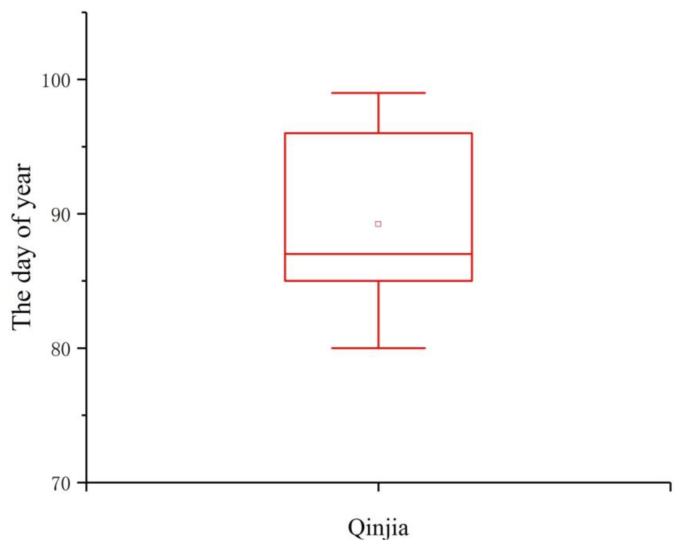
In the original model (Equation (4)), the snowmelt factor in North America reached the maximum on June 21—that is, the 173th day of the year. At this time, reached the maximum. Through a statistical analysis of the box plot (Figure 3), the mean value or the 89th day of the year is the snowmelt starting date—that is, March 30 in our study area (Table 1). According to the principle that the snowmelt factor should be the maximum value of 1 on the 89th day, we optimized the internal parameter of sin to be . The formula was then determined according to the sinusoidal variation law:
The source code was then modified and compiled by the Fortran 90 programming language to replace the run file in the SWAT folder.
3.2. Model Setup and Initial Simulation
A large number of input parameters are required for SWAT [33]. The required database contains two aspects of space and attributes. The collected data include DEM, land-use area, soil type, meteorological data and hydrological data [22]. Details of the information are as follows (Table 2):
For the initial run, the default values in the SWAT model were adopted. The default values of the maximum snowmelt factor and the minimum snowmelt factor were 4.5 in the source code; therefore, no snowmelt module was involved in the initial simulation.
3.3. Sensitivity Analysis
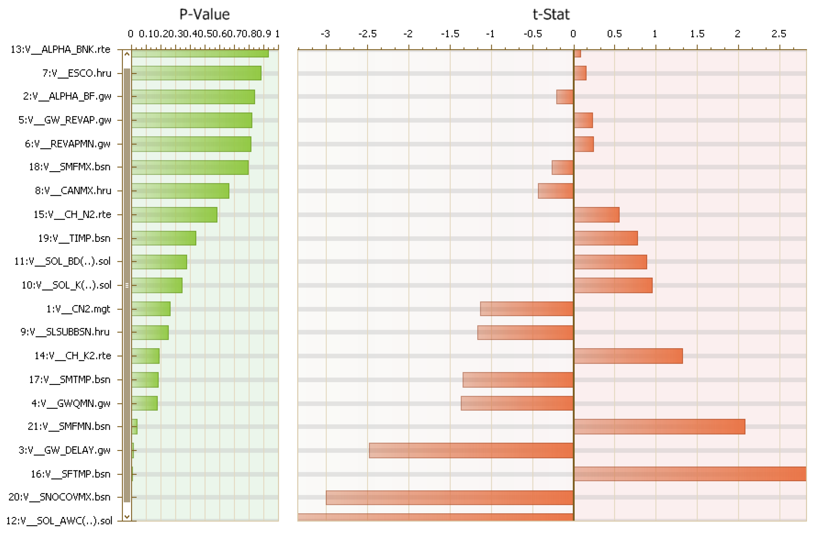
During the operation of the SWAT model, many parameters with different physical concepts are involved. Due to the uniqueness of the regional topography, soil, land-use area, meteorology and other conditions, each basin corresponds to a set of applicable values that are obtained by taking the observed runoff data of the basin as reference. The values of the parameters are adjusted constantly until the runoff simulation results are consistent with the observed results to a certain extent. The sensitivity of the simulation result to a certain input parameter change is then evaluated to determine which parameters have an effect on the runoff generation process of the region—that is, the parameter sensitivity analysis. By adjusting the sensitive parameters and removing the insensitive parameters, the rate of calibration is increased, and a deviation of the adjustment is avoided. In this paper, the new version of SWAT removed the module for parameter sensitivity analysis. Therefore, the combination of software developed by the Swiss Federal Institute of Water Science and Technology, SWAT-CUP, and manual tuning was used for the analysis and calibration of the parameters. This software integrates procedures for many uncertainty algorithms, including SUFI-2 (continuous uncertainty matching), GULE (generalized likelihood uncertainty), and PSO (particle swarm optimization). This software can be directly connected with the SWAT operation results when the sensitivity analysis of the model parameters is carried out. The highly universal SUFI-2 algorithm was selected for this paper, and 21 parameters (Table 3), such as parameters for surface runoff simulation (CN2, ESCO, SOL_AWC, etc.), parameters for baseflow simulation (GW_REVAP, REVAPMN, GWQMN, etc.) parameters for flow process line adjustment (ALPHA_BF, GW_DELAY, etc.) and snowmelt related parameters (SMFMX, SFMMN, SFTMP, SMTMP, TIM level, SONCOVMX, SNO50COV, etc.), were chosen for analysis based on experience and references [39]. Parameter sensitivities were determined using the following multiple regression equation, based on results obtained after running SWAT-CUP 500 times for both models, [26]:
where g is the objective function value, and are regression coefficients, bi is the calibration parameter and m is the number of parameters considered (set to 21). The smaller the P-value is, the larger the absolute value of t-Stat is, and the more sensitive the parameter is [22]. Due to a bug in SWAT-CUP, the SNO50cov.bsn parameter cannot exceed 0.918999. While this factor is important for the snowmelt module, it is listed as a parameter for manual tuning and is not included in the sensitivity analysis.
4. Discussion
4.1. Sensitivity Analysis
The smaller the P-value is, the larger the absolute value of t-Stat is, and the more sensitive the parameter is. As shown in Figure 4, the soil water content is the most sensitive, and the parameters related to snow melting are also sensitive, which further clarifies the necessity for the snowmelt runoff simulation in the study area. Moreover, 21 parameters were found to be sensitive to the simulation results. Therefore, all parameters should participate in the calibration to obtain accurate simulation results.
4.2. Calibration and Validation
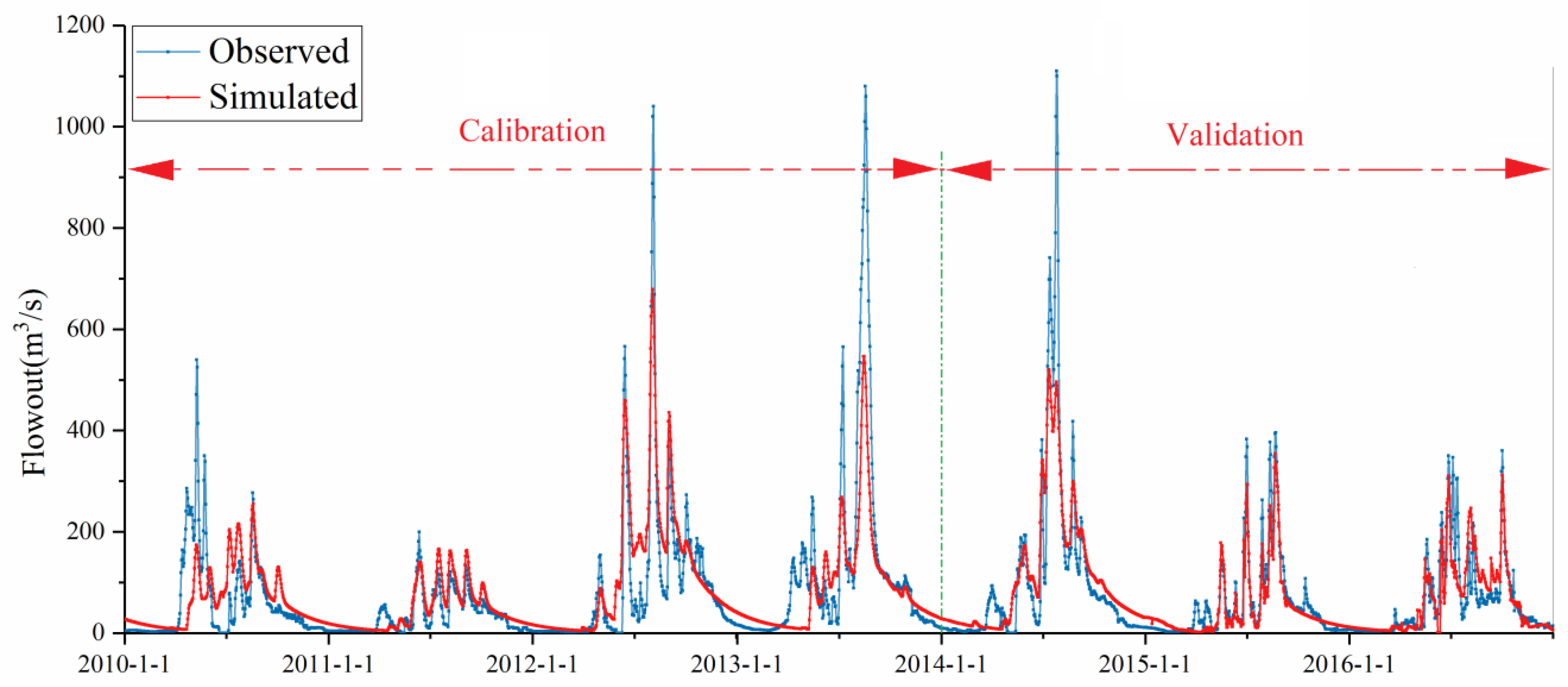
Table 4 shows the optimal results for the parameters. It can be seen from Figure 5 that when the original code model is used to simulate daily runoff, the overall periodicity and peak simulation are relatively good, but during the snowmelt runoff period from March to April, the daily runoff simulation value is relatively low, and sometimes no runoff is generated at all, resulting in poor simulation accuracy without code modification. Therefore, parameters of the snowmelt period should be optimized to increase the simulation accuracy.
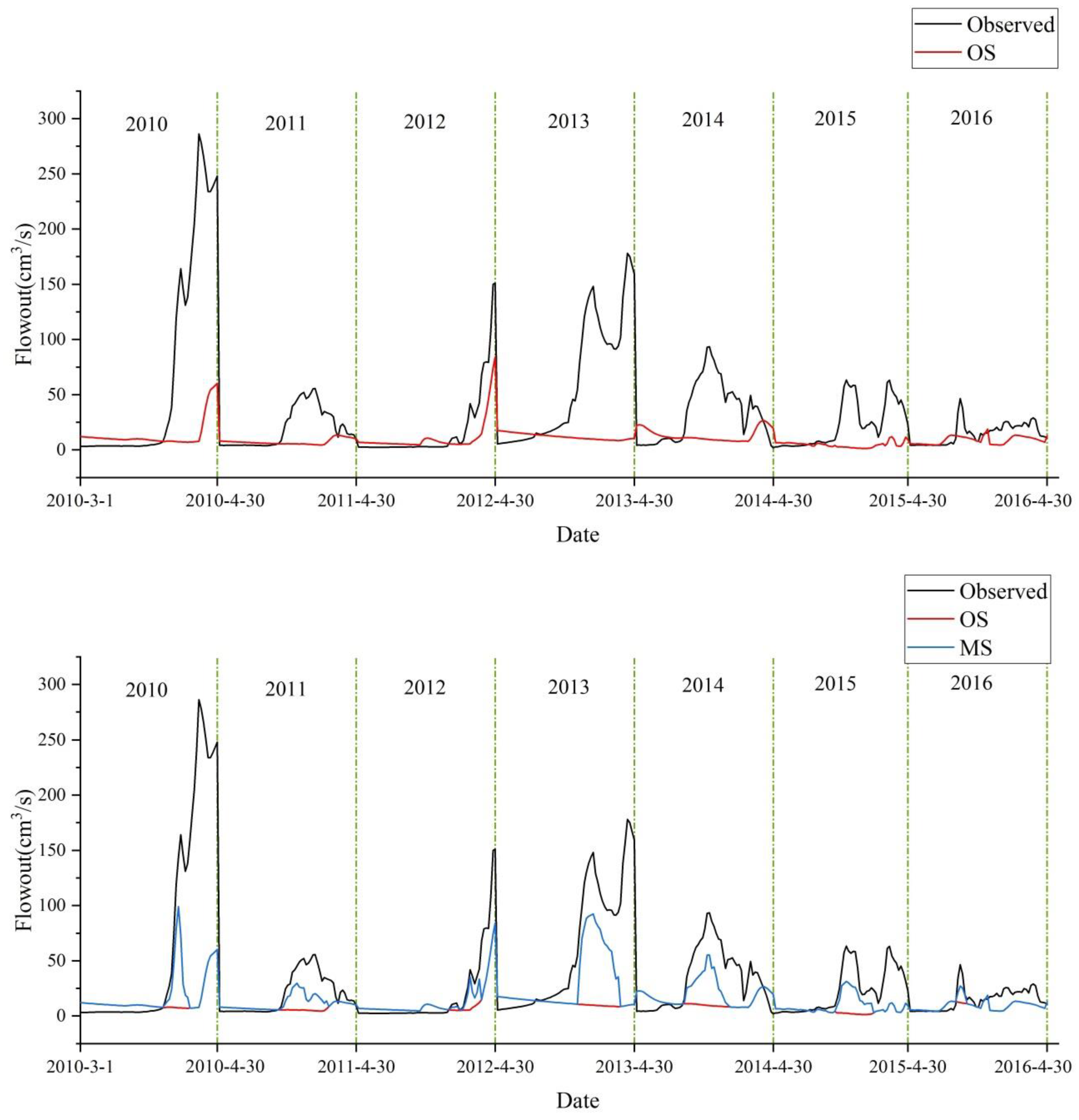
In order to further analyze the simulation effects before and after the parameter optimization, the daily runoff of the snowmelt period from March to April is shown in Figure 6. The peak value of the modified simulated daily flowout was greatly increased, and the period correspondence was further improved, mainly after the snowmelt date. The flowout of the modified simulation from March to April is closer to the observed value, indicating that the modification is effective.
4.3. Model Performance Assessment
From Table 5, the simulation results before and after the modification both indicate a good fit, and the modified result is better than the original result, although the accuracy improvement is not large. Here, we should emphasize that the accuracy of the original parameter is already quite ideal; in this situation, an accuracy improvement is indeed rare and worthwhile. Therefore, the modified simulation exhibits a good periodic improvement in accuracy; however, it still demonstrates a low runoff simulation value, which may be due to the melting of the frozen soil and part of the soil water content entering the river.
4.4. Adequacy of the Modification
The SWAT model can simulate the hydrological process including snowmelt runoff on the river basin scale. The snowmelt runoff simulation is divided into two modules: one is the snowpack module and the other is the snowmelt module, as described in 2.3. The parameters of the snowpack module can be set and adjusted manually on the model operation interface. However, the snowmelt date in the calculation of the snowmelt factor in the snowmelt module is obtained based on the empirical parameters of the development area and is not universal. Therefore, it is necessary to modify the snowmelt starting date based on the actual situation in northeastern China to make the snow melting factor () more accurate. It can be seen that after the modification of the model, the runoff simulation values are closer to the observed values.
5. Conclusions
In high-latitude regions, snowmelt runoff is an important source of spring runoff. The starting date of snowmelt can be statistically and quantitatively determined by a combination of baseflow segmentation and temperature index when data such as snow temperature, terrain, landform, wind speed and sunspots are limited.
When the SWAT model simulates the runoff process within high-latitude regions, since the relevant dates of the maximum and minimum snowmelt factors in the degree-day factor model are taken from the empirical values for North America, the simulated value from the original SWAT model is lower than the actual value or even zero during the early stage of snowmelt. Better simulation results are obtained by recalculating the dates of the maximum and minimum snowmelt factors and modifying the SWAT code to match the actual situation in the study area.
The simulation output of the new SWAT model after modifying the code are still lower than the actual values during the snowmelt runoff. This inconsistency is probably because only the temperature factor is considered in the degree-day factor model, whereas the factors affecting the snowmelt runoff—terrain, radiation, wind speed, vegetation, etc—are not. A multi-factor model can be further explored and improved in future studies by considering the effect of melting frozen soil in the SWAT snowmelt module.
For the application of the SWAT snowmelt model and other models in different regions, there is a profound significance for reference by modifying the background value of the model source code.
Author Contributions
Conceptualization, H.L.; methodology, H.L.; software, Y.L.; validation, G.C.; formal analysis, Y.L.; investigation, Y.L. and G.C.; resources, H.L.; data curation, Y.L. and G.C.; writing—original draft preparation, Y.L.; writing—review and editing, H.L. and G.C.; visualization, G.C.; supervision, H.L.; project administration, H.L.; funding acquisition, H.L. All authors have read and agreed to the published version of the manuscript.
Funding
This research was funded by the key special project of “Efficient Development and Utilization of Water Resources” (Grant number 2017YFC0406005) from the Ministry of Science and Technology of People’s Republic of China.
Acknowledgments
The authors hereby would like to express deep gratitude to the funder for giving support to the research of this paper. The authors would like to thank the editor Doris Cong and the anonymous reviewers for their efforts and constructive comments, which helped improve the manuscript.
Conflicts of Interest
The authors declare no conflict of interest. The funders had no role in the design of the study; in the collection, analyses, or interpretation of data; in the writing of the manuscript, or in the decision to publish the results.
References
- Flanagan, D.C.; Nearing, M.A. USDA-Water Erosion Prediction Project: Hillslope Profile and Watershed Model Documentation. NSERL Report 10; USDA-ARS National Soil Erosion Research Laboratory: West Lafayette, IN, USA, 1995.
- Wang, X.; Melesse, A.M. Evaluation of the Swat Model’s Snowmelt Hydrology in a Northwestern Minnesota Watershed. Trans. Asae 2005, 48, 1359. [Google Scholar] [CrossRef]
- Zeinivand, H.; Smedt, F.D. Hydrological modeling of snow accumulation and melting on river basin scale. Water Resour. Manag. 2009, 23, 2271–2287. [Google Scholar] [CrossRef]
- Shen, Y.J.; Shen, Y.; Fink, M.; Kralisch, S.; Chen, Y.; Brenning, A. Trends and variability in streamflow and snowmelt runoff timing in the southern Tianshan Mountains. J. Hydrol. 2018, 557, 173–181. [Google Scholar] [CrossRef]
- Li, H.Y.; Wang, Y.X.; Jia, L.N.; Wu, Y.N.; Xie, M. Runoff characteristics of the Nen River Basin and its cause. J. Mt. Sci. 2014, 11, 110–118. [Google Scholar] [CrossRef]
- Tuo, Y.; Marcolini, G.; Disse, M.; Chiogna, G. Calibration of snow parameters in SWAT: Comparison of three approaches in the Upper Adige River basin (Italy). Hydrol. Sci. J. 2018, 63, 657–678. [Google Scholar]
- Debele, B.; Srinivasan, R.; Gosain, A. Comparison of process-based and temperature-index snowmelt modeling in SWAT. Water Resour. Manag. 2010, 24, 1065–1088. [Google Scholar] [CrossRef]
- USGS. Precipitation Runoff Modeling System (PRMS); John Wiley & Sons, Ltd.: Hoboken, NJ, USA, 1983; pp. 206–207.
- Band, L.E.; Patterson, P.; Nemani, R.; Running, S.W. Forest ecosystem processes at the watershed scale: Incorporating hillslope hydrology. Agric. For. Meteorol. 1993, 63, 93–126. [Google Scholar] [CrossRef] [Green Version]
- Wood, E.F.; Lettenmaier, D.P.; Zartarian, V.G. A Land Surface Hydrology Parameterization with Sub-Grid Variability for General Circulation Models. J. Geophys. Res. D 1992, 97, 2717–2728. [Google Scholar] [CrossRef]
- Gassman, P.W.; Sadeghi, A.M.; Srinivasan, R. Applications of the SWAT model special section: Overview and insights. J. Environ. Qual. 2014, 43, 1–8. [Google Scholar] [CrossRef]
- Douglasmankin, K.R.; Srinivasan, R.; Arnold, J.G. Soil and Water Assessment Tool (SWAT) Model: Current Developments and Applications. ASABE 2010, 53. [Google Scholar] [CrossRef]
- Gassman, P.W.; Reyes, M.R.; Green, C.H.; Arnold, G.J. The Soil and Water Assessment Tool: Historical Development, Applications, and Future Research Directions. Trans. ASABE 2007, 50, 1211–1250. [Google Scholar] [CrossRef] [Green Version]
- Lévesque, É.; Anctil, F.; Griensven, A.V.; Beauchamp, N. Evaluation of streamflow simulation by SWAT model for two small watersheds under snowmelt and rainfall. Hydrol. Sci. J. 2008, 53, 961–976. [Google Scholar]
- Arnold, J.G.; Srinivasan, R.; Muttiah, R.S.; Williams, J.R. Large area hydrologic modeling and assessment part I: Model development. Jawra J. Am. Water Resour. Assoc. 1998, 34, 73–89. [Google Scholar] [CrossRef]
- Wang, X.; Melesse, A.M. Effects of Statsgo and Ssurgo as Inputs on Swat Model’s Snowmelt Simulation 1. Jawra J. Am. Water Resour. Assoc. 2006, 42, 1217–1236. [Google Scholar] [CrossRef]
- Bouraoui, F.; Grizzetti, B. Modelling mitigation options to reduce diffuse nitrogen water pollution from agriculture. Sci. Total Environ. 2014, 468, 1267–1277. [Google Scholar] [CrossRef]
- Chen, Y.; Marek, G.; Marek, T.; Brauer, D.; Srinivasan, R. Improving SWAT auto-irrigation functions for simulating agricultural irrigation management using long-term lysimeter field data. Environ. Model. Softw. 2018, 99, 25–38. [Google Scholar] [CrossRef]
- Wu, Y.; Liu, J.; Shen, R.; Fu, B. Mitigation of nonpoint source pollution in rural areas: From control to synergies of multi ecosystem services. Sci. Total Environ. 2017, 607, 1376–1380. [Google Scholar] [CrossRef]
- Francesconi, W.; Srinivasan, R.; Pérez-Miñana, E.; Willcock, S.P.; Quintero, M. Using the Soil and Water Assessment Tool (SWAT) to model ecosystem services: A systematic review. J. Hydrol. 2016, 535, 625–636. [Google Scholar] [CrossRef]
- Golmohammadi, G.; Rudra, R.; Dickinson, T.; Goel, P.; Veliz, M. Predicting the temporal variation of flow contributing areas using SWAT. J. Hydrol. 2017, 547, 375–386. [Google Scholar] [CrossRef]
- Liu, R.; Xu, F.; Zhang, P.; Yu, W.; Men, C. Identifying non-point source critical source areas based on multi-factors at a basin scale with SWAT. J. Hydrol. 2016, 533, 379–388. [Google Scholar] [CrossRef]
- Malagò, A.; Efstathiou, D.; Bouraoui, F.; Nikolaidis, N.P.; Franchini, M.; Bidoglio, G.; Kritsotakis, M. Regional scale hydrologic modeling of a karst-dominant geomorphology: The case study of the Island of Crete. J. Hydrol. 2016, 540, 64–81. [Google Scholar] [CrossRef]
- Wang, Y.; Bian, J.; Wang, S.; Tang, J.; Ding, F. Evaluating SWAT Snowmelt Parameters and Simulating Spring Snowmelt Nonpoint Source Pollution in the Source Area of the Liao River. Pol. J. Environ. Stud. 2016, 25. [Google Scholar] [CrossRef]
- Fontaine, T.A.; Cruickshank, T.S.; Arnold, J.G.; Hotchkiss, R.H. Development of a snowfall–snowmelt routine for mountainous terrain for the soil water assessment tool (SWAT). J. Hydrol. 2002, 262, 209–223. [Google Scholar] [CrossRef]
- Qi, J.; Li, S.; Jamieson, R.; Hebb, D.; Xing, Z.; Meng, F.-R. Modifying SWAT with an energy balance module to simulate snowmelt for maritime regions. Environ. Model. Softw. 2017, 93, 146–160. [Google Scholar] [CrossRef]
- Holvoet, K.; Griensven, A.V.; Gevaert, V.; Seuntjens, P.; Vanrolleghem, P.A. Modifications to the SWAT code for modelling direct pesticide losses. Environ. Model. Softw. 2008, 23, 72–81. [Google Scholar] [CrossRef]
- Aksoy, H.; Kurt, I.; Eris, E. Filtered smoothed minima baseflow separation method. J. Hydrol. 2009, 372, 94–101. [Google Scholar] [CrossRef]
- Nathan, R.J.; McMahon, T.A. Evaluation of automated techniques for baseflow and recession analyses. Water Resour. Res. 1990, 26, 1465–1473. [Google Scholar] [CrossRef]
- Sloto, R.A.; Crouse, M.Y. HYSEP, A Computer Program for Streamflow Hydrograph Separation and Analysis; U.S. Geological Survey: Reston, VA, USA, 1996.
- Arnold, J.G.; Moriasi, D.N.; Gassman, P.W.; Abbaspour, K.C.; White, M.J.; Srinivasan, R.; Santhi, C.; Harmel, R.D.; Griensven, A.V.; Liew, M.W.V. SWAT: Model use, calibration, and validation. Trans. Asabe 2012, 55, 1549–1559. [Google Scholar] [CrossRef]
- Neitsch, S.; Arnold, J.; Kiniry, J.; Srinivasan, R.; Williams, J. Soil and water assessment tool user’s manual version 2000. Gsl. Rep. 2002, 202, 2–6. [Google Scholar]
- Srinivasan, R.; Zhang, X.; Arnold, J. SWAT ungauged: Hydrological budget and crop yield predictions in the Upper Mississippi River Basin. Trans. Asabe 2010, 53, 1533–1546. [Google Scholar] [CrossRef]
- Holzworth, D.P.; Snow, V.; Janssen, S.; Athanasiadis, I.N.; Donatelli, M.; Hoogenboom, G.; White, J.W.; Thorburn, P. Agricultural production systems modelling and software: Current status and future prospects. Environ. Model. Softw. 2015, 72, 276–286. [Google Scholar] [CrossRef]
- Abbaspour, K.C. SWAT-CUP 2012: SWAT Calibration and Uncertainty Programs—A User Manual; Eawag: Dübendorf, Switzerland, 2013. [Google Scholar]
- Dhami, B.; Himanshu, S.K.; Pandey, A.; Gautam, A.K. Evaluation of the SWAT model for water balance study of a mountainous snowfed river basin of Nepal. Environ. Earth Sci. 2018, 77, 21. [Google Scholar] [CrossRef]
- Nash, J.E.; Sutcliffe, J.V. River flow forecasting through conceptual models part I—A discussion of principles. J. Hydrol. 1970, 10, 282–290. [Google Scholar] [CrossRef]
- Moriasi, D.N.; Arnold, J.G.; Liew, M.W.V.; Bingner, R.L.; Harmel, R.D.; Veith, T.L. Model Evaluation Guidelines for Systematic Quantification of Accuracy in Watershed Simulations. Trans. Asabe 2007, 50, 885–900. [Google Scholar] [CrossRef]
- Singh, V.; Bankar, N.; Salunkhe, S.S.; Bera, A.K.; Sharma, J. Hydrological stream flow modelling on Tungabhadra catchment: Parameterization and uncertainty analysis using SWAT CUP. Curr. Sci. 2013, 104, 1187–1199. [Google Scholar]
Figure 1.
Location of the study area.

Figure 2.
Baseflow segmentation index and temperature trend of the Qinjia station (Green arrows represent snowmelt starting date, T-max is the daily maximum temperature and T-min is the daily minimum temperature).
Figure 2.
Baseflow segmentation index and temperature trend of the Qinjia station (Green arrows represent snowmelt starting date, T-max is the daily maximum temperature and T-min is the daily minimum temperature).

Figure 3.
Distribution of snow melting days

Figure 4.
Sensitivity analysis results.

Figure 5.
Observed and simulated daily runoff at Qinjia Station before code modification.

Figure 6.
Comparison of two simulation results and observed values (Date from March 1 to April 30 of each year from 2010 to 2016; OS represents the original simulation and MS represents the modified simulation).
Figure 6.
Comparison of two simulation results and observed values (Date from March 1 to April 30 of each year from 2010 to 2016; OS represents the original simulation and MS represents the modified simulation).


Table 1.
Qinjia snowmelt dates statistical results.
| N Total | Mean | Standard Deviation | Sum | Minimum | Median | Maximum |
|---|---|---|---|---|---|---|
| 9 | 89 | 6.667 | 803 | 80 | 89 | 99 |
Table 2.
Basic data for the model.
| Data | Range Accuracy | Data Sources |
|---|---|---|
| Digital elevation model | STRM 90 m | http://www.gscloud.cn/ |
| Soil maps | 1:1000000 | Harmonized world soil database |
| Land use/cover | 1:100000 | http://www.resdc.cn/data.aspx?DATAID=99 |
| Weather data | CMADS (2008–2016) | http://westdc.westgis.ac.cn |
| Runoff | 2008–2016 | Hydrographic office |
Table 3.
Physical meaning and range of relevant parameters.
| Parameter_Name | File | Physical Significance | Range | Unit |
|---|---|---|---|---|
| CN2 | mgt | SCS runoff curve number | 35–98 | dimensionless |
| ALPHA_BF | gw | Baseflow alpha factor | 0–1 | days |
| GW_DELAY | gw | Groundwater delay | 0–500 | days |
| GWQMN | gw | Threshold depth of water in the shallow aquifer required for return flow to occur | 0–5000 | mm H2O |
| GW_REVAP | gw | Groundwater “revap” coefficient | 0.02–0.2 | dimensionless |
| REVAPMN | gw | Threshold depth of water in the shallow aquifer for “revap” to occur | 0–500 | mm H2O |
| ESCO | hru | Soil evaporation compensation factor | 0–1 | dimensionless |
| CANMX | hru | Maximum canopy storage | 0–100 | mm H2O |
| SLSUBBSN | hru | Average slope length | 10–150 | m |
| SOL_K(..) | sol | Saturated hydraulic conductivity | 0–2000 | mm/hr |
| SOL_BD(..) | sol | Moist bulk density | 0.9–2.5 | g/cm3 |
| SOL_AWC(..) | sol | Available water capacity of the soil layer | 0–1 | mm H2O/mm soil |
| ALPHA_BNK | rte | Baseflow alpha factor for bank storage | 0–1 | days |
| CH_K2 | rte | Effective hydraulic conductivity in main channel alluvium | −500.01 | mm/hr |
| CH_N2 | rte | Manning’s “n” value for the main channel | −0.31 | dimensionless |
| SFTMP | bsn | Snowfall temperature | −40 | °C |
| SMTMP | bsn | Snow melt base temperature | −40 | °C |
| SMFMX | bsn | Maximum melt rate for snow during year (occurs on summer solstice) | 0–20 | mm H2O/°C day |
| TIMP | bsn | Snowpack temperature lag factor | 0–1 | dimensionless |
| SNOCOVMX | bsn | Minimum snow water content that corresponds to 100% snow cover | 0–500 | mm H2O |
| SMFMN | bsn | Minimum melt rate for snow during the year (occurs on winter solstice) | 0–20 | mm H2O/°C day |
| SNO50COV | bsn | Minimum snow water content that corresponds to 50% snow cover | 0–500 | dimensionless |
Table 4.
Parameter calibration results.
| Parameter_Name | file | Assignment | Fitted_Value | Unit |
|---|---|---|---|---|
| CN2 | mgt | v | 35.2326 | dimensionless |
| ALPHA_BF | gw | v | 0.502689 | days |
| GW_DELAY | gw | v | 65.853645 | days |
| GWQMN | gw | v | 841.039673 | mm H2O |
| GW_REVAP | gw | v | 0.098768 | dimensionless |
| REVAPMN | gw | v | 54.239353 | mm H2O |
| ESCO | hru | v | 0.157893 | dimensionless |
| CANMX | hru | v | 41.954502 | mm H2O |
| SLSUBBSN | hru | v | 42.100601 | m |
| SOL_K(..) | sol | v | 1785.92395 | mm/hr |
| SOL_BD(..) | sol | v | 1.465848 | g/cm3 |
| SOL_AWC(..) | sol | v | −0.101126 | mm H2O/mm soil |
| ALPHA_BNK | rte | v | 0.503674 | days |
| CH_K2 | rte | v | 344.855682 | mm/hr |
| CH_N2 | rte | v | 0.219884 | dimensionless |
| SFTMP | bsn | v | 4.236598 | °C |
| SMTMP | bsn | v | 8.508638 | °C |
| SMFMX | bsn | v | 6.828101 | mm H2O/°C day |
| TIMP | bsn | v | 0.545052 | dimensionless |
| SNOCOVMX | bsn | v | 79.400223 | mm H2O |
| SMFMN | bsn | v | 15.326536 | mm H2O/°C day |
| SNO50COV | bsn | v | 0.5 | dimensionless |
Table 5.
Evaluation of simulation.
| Annual | Mode Evaluation Statistics | Original | Modification | ||
| Calibration (2010–2013) | Validation (2014–2016) | Calibration (2010–2013) | Validation (2014–2016) | ||
| NSE | 0.6926 | 0.70243 | 0.70253 | 0.813204 | |
| R2 | 0.7661 | 0.785 | 0.784 | 0.791 | |
| PBIAS | −0.01732 | 0.0206 | −0.03299 | 0.011 | |
| Snowmelt from March to April | Mode Evaluation Statistics | Original | Modification | ||
| Calibration (2010–2013) | Validation (2014–2016) | Calibration (2010–2013) | Validation (2014–2016) | ||
| NSE | −0.09896 | −3.396 | 0.141611 | 0.207441 | |
| R2 | 0.225 | 0.013 | 0.347 | 0.231 | |
| PBIAS | 0.73338 | 0.620122 | 0.557087 | 0.443954 | |
© 2020 by the authors. Licensee MDPI, Basel, Switzerland. This article is an open access article distributed under the terms and conditions of the Creative Commons Attribution (CC BY) license (http://creativecommons.org/licenses/by/4.0/).
Share and Cite
MDPI and ACS Style
Liu, Y.; Cui, G.; Li, H. Optimization and Application of Snow Melting Modules in SWAT Model for the Alpine Regions of Northern China. Water 2020, 12, 636. https://doi.org/10.3390/w12030636
AMA Style
Liu Y, Cui G, Li H. Optimization and Application of Snow Melting Modules in SWAT Model for the Alpine Regions of Northern China. Water. 2020; 12(3):636. https://doi.org/10.3390/w12030636
Chicago/Turabian StyleLiu, Yan, Geng Cui, and Hongyan Li. 2020. "Optimization and Application of Snow Melting Modules in SWAT Model for the Alpine Regions of Northern China" Water 12, no. 3: 636. https://doi.org/10.3390/w12030636
Note that from the first issue of 2016, this journal uses article numbers instead of page numbers. See further details here.