Disentangling the Effects of Multiple Stressors on Large Rivers Using Benthic Invertebrates—A Study of Southeastern European Large Rivers with Implications for Management


Abstract
:1. Introduction
2. Materials and Methods
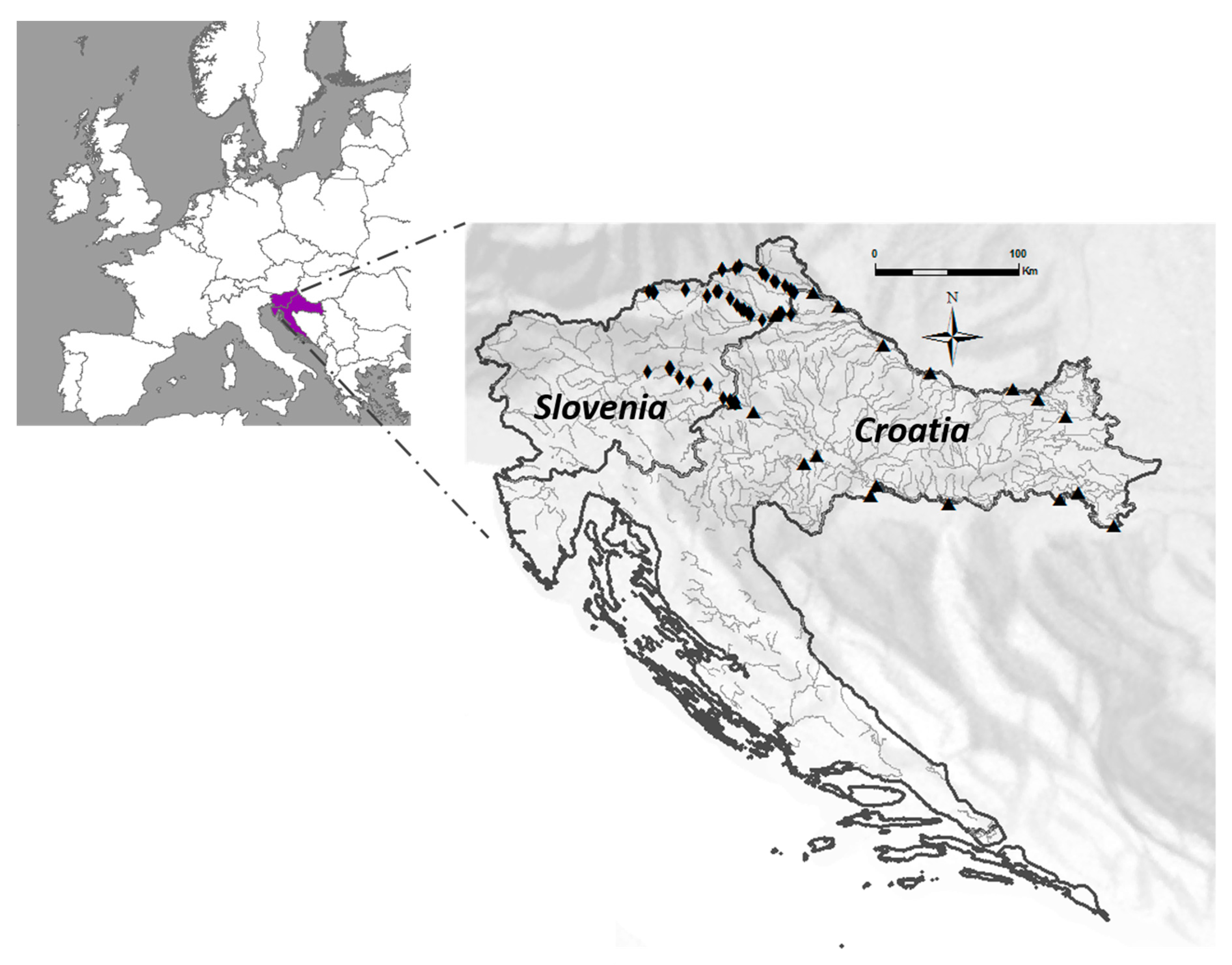
2.1. Study Area
2.2. Environmental Variables
2.3. Benthic Invertebrates
2.4. Data Analyses
3. Results
3.1. Relationships between the Variables
3.2. Benthic Invertebrate Response to Environmental Variables
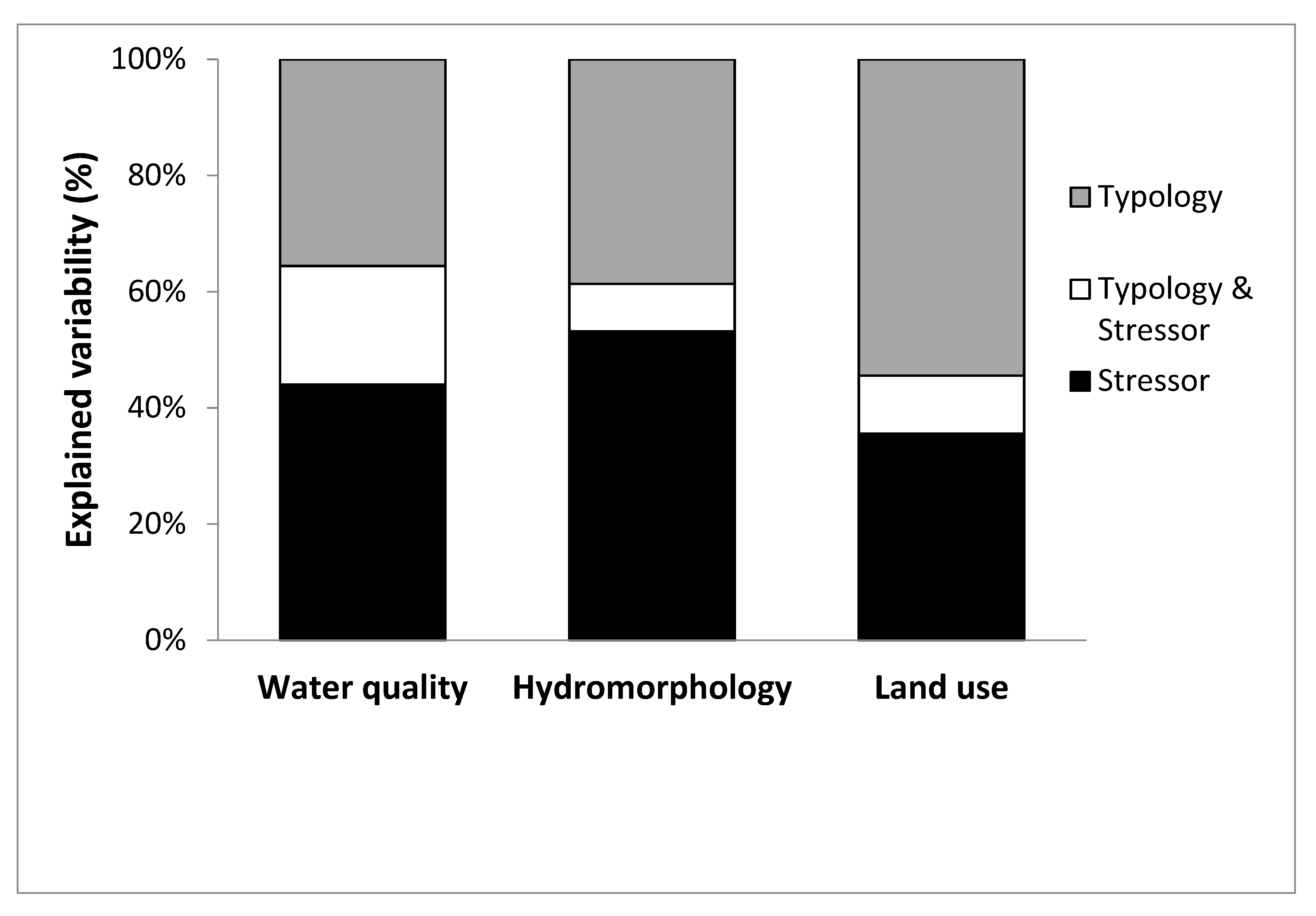
3.3. Variance Partitioning between Typology and Stressor-Groups
3.4. Variance Partitioning of Three Stressor Variable Groups of Environmental Variables
4. Discussion
5. Conclusions
- We disentangled the specific effects of hydromorphology, water quality, and land use using benthic invertebrate assemblages.
- Joint effects of stressors and natural factors on benthic invertebrate assemblages depend on the stressor group.
- Stressors proved to be the dominant factors in shaping benthic invertebrate assemblages of Southeastern Europe large rivers. Effects of hydromorphology dominated over water quality and land use effects, though these were still substantial. Thus, all major stressors need to be addressed and their effects determined for the implementation of the sustainable river basin management strategies.
- Management agencies in Southeastern Europe need to change their paradigm from river water quality to the ecological quality of the river ecosystem, thereby supporting activities that will prevent large river deterioration.
Author Contributions
Funding
Acknowledgments
Conflicts of Interest
Appendix A

| River | Site | No. Samples | Latitude | Longitude |
|---|---|---|---|---|
| Drava | Belišće | 1 | 45.6924 | 18.4187 |
| Drava | Borl | 1 | 46.3687 | 15.9903 |
| Drava | Botovo | 2 | 46.2592 | 16.9273 |
| Drava | Bresternica | 1 | 46.5678 | 15.5971 |
| Drava | Brezno | 2 | 46.5949 | 15.3154 |
| Drava | Donji Miholjac | 1 | 45.7831 | 18.2070 |
| Drava | Dravograd | 3 | 46.5884 | 15.0251 |
| Drava | Frankovci | 2 | 46.3974 | 16.1687 |
| Drava | Grabe | 2 | 46.3919 | 16.2542 |
| Drava | Krčevina pri Ptuju | 3 | 46.4403 | 15.8333 |
| Drava | Križovljan Grad | 1 | 46.3846 | 16.1157 |
| Drava | Mariborski otok | 4 | 46.5677 | 15.6137 |
| Drava | Markovci | 2 | 46.4106 | 15.8891 |
| Drava | Ormož | 3 | 46.3863 | 16.1206 |
| Drava | Ptuj | 2 | 46.4178 | 15.8690 |
| Drava | Pušenci | 2 | 46.4021 | 16.1571 |
| Drava | Ranca | 1 | 46.4108 | 15.8883 |
| Drava | Ruše | 3 | 46.5458 | 15.5083 |
| Drava | Slovenja vas | 1 | 46.4441 | 15.8130 |
| Drava | Starše | 1 | 46.4754 | 15.7702 |
| Drava | Terezino Polje | 1 | 45.9425 | 17.4822 |
| Drava | Tribej | 2 | 46.6020 | 14.9783 |
| Drava | Višnjevac | 1 | 45.5762 | 18.6452 |
| Drava | Zgornji Duplek | 2 | 46.5176 | 15.7143 |
| Kupa | Brest | 2 | 45.4424 | 16.2429 |
| Mura | Bunčani | 1 | 46.5985 | 16.1484 |
| Mura | Ceršak | 5 | 46.7062 | 15.6665 |
| Mura | Gibina-Brod | 2 | 46.5236 | 16.3391 |
| Mura | Goričan | 1 | 46.4154 | 16.7029 |
| Mura | Gornja Bistrica | 1 | 46.5404 | 16.2714 |
| Mura | Konjišče | 2 | 46.7193 | 15.8206 |
| Mura | Mali Bakovci | 1 | 46.6074 | 16.1280 |
| Mura | Mele | 2 | 46.6495 | 16.0504 |
| Mura | Melinci | 1 | 46.5719 | 16.2227 |
| Mura | Mota | 4 | 46.5504 | 16.2424 |
| Mura | Peklenica | 1 | 46.5105 | 16.4753 |
| Mura | Petanjci | 1 | 46.6492 | 16.0504 |
| Mura | Trate | 1 | 46.7070 | 15.7855 |
| Sava | Boštanj | 1 | 46.0110 | 15.2926 |
| Sava | Brestanica | 2 | 46.9873 | 15.4657 |
| Sava | Brežice | 1 | 45.8981 | 15.5903 |
| Sava | Davor | 2 | 45.1088 | 17.5247 |
| Sava | Dolenji Leskovec | 1 | 45.9860 | 15.4516 |
| Sava | Drenje | 1 | 45.8620 | 15.6924 |
| Sava | Galdovo | 1 | 45.4833 | 16.3935 |
| Sava | Jasenovac | 1 | 45.2633 | 16.8998 |
| Sava | Jesenice na Dolenjskem | 6 | 45.8609 | 15.6921 |
| Sava | Mošenik | 1 | 46.0922 | 14.9228 |
| Sava | Podgračeno | 2 | 45.8759 | 15.6500 |
| Sava | Podkraj | 3 | 46.1115 | 15.1158 |
| Sava | Račinovci | 1 | 44.8501 | 18.9661 |
| Sava | Slavonski Šamac | 1 | 45.0582 | 18.5093 |
| Sava | Suhadol | 3 | 46.1057 | 15.1253 |
| Sava | Vrhovo | 4 | 46.0445 | 15.2089 |
| Sava | Zagreb-Jankomir | 1 | 45.7911 | 15.8526 |
| Sava | Županja | 1 | 45.0685 | 18.6745 |
| Una | Hrvatska Dubica | 3 | 45.1900 | 16.7894 |
Appendix B
| Higher Taxon | Taxon |
|---|---|
| Turbellaria | Dendrocoelum album |
| Turbellaria | Dendrocoelum lacteum |
| Turbellaria | Dugesia gonocephala |
| Turbellaria | Dugesia lugubris/polychroa |
| Turbellaria | Dugesia lugubris |
| Turbellaria | Dugesia tigrina |
| Turbellaria | Phagocata sp. |
| Turbellaria | Planaria torva |
| Turbellaria | Polycelis nigra/tenuis |
| Nematoda | Nematoda Gen. sp. |
| Oligochaeta | Enchytraeidae Gen. sp. |
| Oligochaeta | Haplotaxis gordioides |
| Oligochaeta | Eiseniella tetraedra |
| Oligochaeta | Lumbriculidae Gen. sp. |
| Oligochaeta | Lumbriculus variegatus |
| Oligochaeta | Rhynchelmis sp. |
| Oligochaeta | Stylodrilus heringianus |
| Oligochaeta | Stylodrilus sp. |
| Oligochaeta | Chaetogaster sp. |
| Oligochaeta | Dero sp. |
| Oligochaeta | Nais sp. |
| Oligochaeta | Ophidonais serpentina |
| Oligochaeta | Pristina sp. |
| Oligochaeta | Stylaria lacustris |
| Oligochaeta | Uncinais uncinata |
| Oligochaeta | Vejdovskiella comata |
| Oligochaeta | Vejdovskiella sp. |
| Oligochaeta | Propappus volki |
| Oligochaeta | Aulodrilus pluriseta |
| Oligochaeta | Branchiura sowerbyi |
| Oligochaeta | Peloscolex sp. |
| Oligochaeta | Peloscolex velutina |
| Oligochaeta | Tubificidae juv without setae |
| Oligochaeta | Tubificidae juv with setae |
| Hirudinea | Dina punctata |
| Hirudinea | Erpobdella nigricollis |
| Hirudinea | Erpobdella octoculata |
| Hirudinea | Erpobdella sp. |
| Hirudinea | Erpobdella testacea |
| Hirudinea | Erpobdella vilnensis |
| Hirudinea | Trocheta bykowskii |
| Hirudinea | Alboglossiphonia heteroclita |
| Hirudinea | Glossiphonia complanata |
| Hirudinea | Glossiphonia concolor |
| Hirudinea | Glossiphonia nebulosa |
| Hirudinea | Glossiphonia paludosa |
| Hirudinea | Glossiphonia sp. |
| Hirudinea | Glossiphonia verrucata |
| Hirudinea | Helobdella stagnalis |
| Hirudinea | Hemiclepsis marginata |
| Hirudinea | Theromyzon tessulatum |
| Hirudinea | Haemopis sanguisuga |
| Hirudinea | Piscicola geometra |
| Hirudinea | Piscicola haranti |
| Gastropoda | Acroloxus lacustris |
| Gastropoda | Ancylus fluviatilis |
| Gastropoda | Bithynia tentaculata |
| Gastropoda | Bithynia sp. |
| Gastropoda | Borysthenia naticina |
| Gastropoda | Lithoglyphus naticoides |
| Gastropoda | Potamopyrgus antipodarum |
| Gastropoda | Sadleriana sp. |
| Gastropoda | Radix auricularia |
| Gastropoda | Radix balthica/labiata |
| Gastropoda | Radix balthica |
| Gastropoda | Radix labiata |
| Gastropoda | Esperiana acicularis |
| Gastropoda | Esperiana esperi |
| Gastropoda | Holandriana holandrii |
| Gastropoda | Theodoxus danubialis |
| Gastropoda | Theodoxus transversalis |
| Gastropoda | Physa fontinalis |
| Gastropoda | Physella acuta |
| Gastropoda | Gyraulus albus |
| Gastropoda | Gyraulus crista |
| Gastropoda | Planorbis carinatus |
| Gastropoda | Valvata cristata |
| Gastropoda | Valvata piscinalis |
| Gastropoda | Viviparus viviparus |
| Bivalvia | Dreissena polymorpha |
| Bivalvia | Musculium lacustre |
| Bivalvia | Pisidium sp. |
| Bivalvia | Sphaerium corneum |
| Bivalvia | Sphaerium sp. |
| Bivalvia | Sinanodonta woodiana |
| Bivalvia | Unio crassus |
| Bivalvia | Unio pictorum |
| Bivalvia | Unio tumidus |
| Bivalvia | Corbicula fluminea |
| Arachnida | Hydrachnidia Gen. sp. |
| Amphipoda | Synurella ambulans |
| Amphipoda | Gammarus fossarum |
| Amphipoda | Gammarus roeselii |
| Amphipoda | Corophium curvispinum |
| Amphipoda | Dikerogammarus haemobaphes |
| Amphipoda | Dikerogammarus villosus |
| Amphipoda | Niphargus sp. |
| Isopoda | Asellus aquaticus |
| Isopoda | Jaera istri |
| Ephemeroptera | Baetis buceratus |
| Ephemeroptera | Nigrobaetis digitatus |
| Ephemeroptera | Baetis fuscatus |
| Ephemeroptera | Baetis fuscatus/scambus |
| Ephemeroptera | Baetis liebenauae |
| Ephemeroptera | Baetis lutheri |
| Ephemeroptera | Baetis rhodani |
| Ephemeroptera | Baetis scambus |
| Ephemeroptera | Baetis sp. |
| Ephemeroptera | Baetis vardarensis |
| Ephemeroptera | Baetis vernus |
| Ephemeroptera | Baetis buceratus/vernus |
| Ephemeroptera | Centroptilum luteolum |
| Ephemeroptera | Centroptilum sp. |
| Ephemeroptera | Cloeon dipterum |
| Ephemeroptera | Caenis sp. |
| Ephemeroptera | Brachycercus sp. |
| Ephemeroptera | Serratella ignita |
| Ephemeroptera | Ephemerella notata |
| Ephemeroptera | Ephemerella mucronata |
| Ephemeroptera | Torleya major |
| Ephemeroptera | Ephemera danica |
| Ephemeroptera | Ephemera sp. |
| Ephemeroptera | Ecdyonurus sp. |
| Ephemeroptera | Epeorus sylvicola |
| Ephemeroptera | Heptagenia sp. |
| Ephemeroptera | Heptagenia sulphurea |
| Ephemeroptera | Rhithrogena sp. |
| Ephemeroptera | Habroleptoides confusa |
| Ephemeroptera | Habrophlebia fusca |
| Ephemeroptera | Paraleptophlebia submarginata |
| Ephemeroptera | Oligoneuriella rhenana |
| Ephemeroptera | Potamanthus luteus |
| Ephemeroptera | Siphlonurus aestivalis |
| Ephemeroptera | Siphlonurus lacustris |
| Ephemeroptera | Siphlonurus sp. |
| Plecoptera | Chloroperla sp. |
| Plecoptera | Xanthoperla apicalis |
| Plecoptera | Capnia sp. |
| Plecoptera | Leuctra sp. |
| Plecoptera | Nemoura sp. |
| Plecoptera | Nemurella pictetii |
| Plecoptera | Protonemura sp. |
| Plecoptera | Dinocras cephalotes |
| Plecoptera | Perla sp. |
| Plecoptera | Marthamea vitripennis |
| Plecoptera | Isoperla sp. |
| Plecoptera | Perlodes sp. |
| Plecoptera | Brachyptera sp. |
| Plecoptera | Taeniopteryx nebulosa |
| Odonata | Calopteryx splendens |
| Odonata | Cercion lindenii |
| Odonata | Enallagma cyathigerum |
| Odonata | Ischnura elegans |
| Odonata | Coenagrionidae Gen. sp. |
| Odonata | Cordulegaster bidentata |
| Odonata | Cordulegaster heros |
| Odonata | Gomphus sp. |
| Odonata | Gomphus vulgatissimus |
| Odonata | Gomphus flavipes |
| Odonata | Onychogomphus forcipatus |
| Odonata | Ophiogomphus cecilia |
| Odonata | Orthetrum brunneum |
| Odonata | Platycnemis pennipes |
| Heteroptera | Aphelocheirus aestivalis |
| Heteroptera | Corixinae Gen. sp. |
| Heteroptera | Micronecta sp. |
| Megaloptera | Sialis fuliginosa |
| Megaloptera | Sialis lutaria |
| Megaloptera | Sialis nigripes |
| Hymenoptera | Agriotypus armatus |
| Coleoptera | Bidessus sp. Ad. |
| Coleoptera | Platambus maculatus Ad. |
| Coleoptera | Elmis sp. Ad. |
| Coleoptera | Elmis sp. Lv. |
| Coleoptera | Esolus sp. Ad. |
| Coleoptera | Esolus sp. Lv. |
| Coleoptera | Limnius sp. Ad. |
| Coleoptera | Limnius sp. Lv. |
| Coleoptera | Normandia nitens Ad. |
| Coleoptera | Oulimnius sp. Ad. |
| Coleoptera | Oulimnius sp. Lv. |
| Coleoptera | Riolus sp. Ad. |
| Coleoptera | Riolus sp. Lv. |
| Coleoptera | Stenelmis canaliculata Ad. |
| Coleoptera | Orectochilus villosus Lv. |
| Coleoptera | Haliplus sp. Ad. |
| Coleoptera | Haliplus sp. Lv. |
| Coleoptera | Helophorus sp. Ad. |
| Coleoptera | Hydraena sp. Ad. |
| Coleoptera | Ochthebius sp. Ad. |
| Trichoptera | Brachycentrus montanus |
| Trichoptera | Brachycentrus subnubilus |
| Trichoptera | Ecnomus tenellus |
| Trichoptera | Agapetus sp. |
| Trichoptera | Agapetus laniger |
| Trichoptera | Glossosoma boltoni |
| Trichoptera | Glossosoma conformis |
| Trichoptera | Glossosoma intermedium |
| Trichoptera | Goera pilosa |
| Trichoptera | Silo nigricornis |
| Trichoptera | Silo piceus |
| Trichoptera | Cheumatopsyche lepida |
| Trichoptera | Hydropsyche bulbifera |
| Trichoptera | Hydropsyche bulgaromanorum |
| Trichoptera | Hydropsyche contubernalis |
| Trichoptera | Hydropsyche incognita |
| Trichoptera | Hydropsyche modesta |
| Trichoptera | Hydropsyche ornatula |
| Trichoptera | Hydropsyche pellucidula |
| Trichoptera | Hydropsyche siltalai |
| Trichoptera | Hydropsyche sp. |
| Trichoptera | Hydroptila sp. |
| Trichoptera | Orthotrichia sp. |
| Trichoptera | Lepidostoma hirtum |
| Trichoptera | Athripsodes albifrons |
| Trichoptera | Athripsodes cinereus |
| Trichoptera | Athripsodes sp. |
| Trichoptera | Ceraclea annulicornis |
| Trichoptera | Ceraclea dissimilis |
| Trichoptera | Mystacides azurea |
| Trichoptera | Mystacides longicornis |
| Trichoptera | Mystacides nigra |
| Trichoptera | Oecetis lacustris |
| Trichoptera | Oecetis notata |
| Trichoptera | Setodes punctatus |
| Trichoptera | Setodes sp. |
| Trichoptera | Anabolia furcata |
| Trichoptera | Chaetopteryx sp. |
| Trichoptera | Halesus digitatus |
| Trichoptera | Halesus radiatus |
| Trichoptera | Limnephilinae Gen. sp. |
| Trichoptera | Limnephilus extricatus |
| Trichoptera | Potamophylax rotundipennis |
| Trichoptera | Potamophylax sp. |
| Trichoptera | Philopotamus sp. |
| Trichoptera | Cyrnus trimaculatus |
| Trichoptera | Polycentropus flavomaculatus |
| Trichoptera | Lype reducta |
| Trichoptera | Psychomyia pusilla |
| Trichoptera | Tinodes sp. |
| Trichoptera | Rhyacophila s. str. sp. |
| Trichoptera | Notidobia ciliaris |
| Trichoptera | Sericostoma sp. |
| Diptera | Limnophora sp. |
| Diptera | Lispe sp. |
| Diptera | Atherix ibis |
| Diptera | Ibisia marginata |
| Diptera | Ibisia sp. |
| Diptera | Liponeura sp. |
| Diptera | Ceratopogoninae Gen. sp. |
| Diptera | Dasyhelea sp. |
| Diptera | Brillia bifida |
| Diptera | Chironomini Gen. sp. |
| Diptera | Chironomus obtusidens-Gr. |
| Diptera | Chironomus plumosus-Gr. |
| Diptera | Chironomus thummi-Gr. |
| Diptera | Chironomus plumosus |
| Diptera | Chironomus sp. |
| Diptera | Corynoneura sp. |
| Diptera | Orthocladiinae Gen. sp. |
| Diptera | Diamesinae Gen. sp. |
| Diptera | Monodiamesa sp. |
| Diptera | Orthocladiinae Gen. sp. |
| Diptera | Paratendipes sp. |
| Diptera | Potthastia longimana-Gr. |
| Diptera | Procladius sp. |
| Diptera | Prodiamesa olivacea |
| Diptera | Prodiamesa rufovittata |
| Diptera | Tanypodinae Gen. sp. |
| Diptera | Tanytarsini Gen. sp. |
| Diptera | Thienemanniella sp. |
| Diptera | Dolichopodidae Gen. sp. |
| Diptera | Clinocerinae Gen. sp. |
| Diptera | Hemerodromiinae Gen. sp. |
| Diptera | Antocha sp. |
| Diptera | Chioneinae Gen. sp. |
| Diptera | Hexatoma sp. |
| Diptera | Limnophilinae Gen. sp. |
| Diptera | Limoniinae Gen. sp. |
| Diptera | Dicranota sp. |
| Diptera | Pedicia sp. |
| Diptera | Psychodidae Gen. sp. |
| Diptera | Psychodidae Gen. sp. |
| Diptera | Psychodidae Gen. sp. |
| Diptera | Ptychoptera sp. |
| Diptera | Prosimulium sp. |
| Diptera | Simulium sp. |
| Diptera | Syrphidae Gen. sp. |
| Diptera | Chrysops sp. |
| Diptera | Tabanus sp. |
| Diptera | Tipula sp. |
| Lepidoptera | Nymphula stagnata |
Appendix C
| Depth_Mean | C_Size | Slope | Altitude | Substrat_Code | |
|---|---|---|---|---|---|
| Depth_mean | 0.494** | −0.613** | −0.373** | ||
| C_size | 0.494** | −0.405** | −0.465** | ||
| slope | −0.613** | −0.405** | 0.299** | 0.337** | |
| altitude | 0.299** | 0.499** | |||
| substrat_code | −0.373** | −0.465** | 0.337** | 0.499** | |
| T_med | 0.197* | −0.278** | −0.361** | ||
| pH_med | −0.277** | ||||
| cond_med | −0.461** | −0.418** | −0.631** | ||
| DO_med | −0.257** | −0.209* | |||
| DOsat_med | |||||
| TSS_med | 0.329** | 0.391** | −0.233* | −0.293** | |
| KPK_Cmed | −0.313** | −0.278** | −0.277** | ||
| BPK5_med | −0.221* | −0.443** | −0.248* | ||
| PO4_P_med | −0.505** | −0.561** | 0.243* | −0.353** | |
| Ntot_med | −0.643** | −0.427** | 0.401** | ||
| NH4_N_med | −0.213* | −0.404** | |||
| NO2_N_med | −0.613** | −0.573** | 0.461** | 0.439** | |
| NO3_N_med | −0.607** | −0.444** | 0.414** | ||
| Q | 0.591** | 0.564** | −0.509** | −0.198* | −0.450** |
| Qnp | 0.571** | 0.520** | −0.513** | −0.250* | −0.488** |
| Qs | 0.544** | 0.443** | −0.546** | −0.378** | −0.490** |
| Qvk | 0.336** | −0.382** | −0.487** | −0.383** | |
| RHQ | −0.652** | 0.350** | −0.330** | ||
| RHM | 0.299** | 0.254** | |||
| HLM | −0.395** | −0.685** | −0.437** | ||
| HMM | −0.392** | −0.582** | −0.410** | ||
| HQM | −0.408** | −0.625** | −0.408** | ||
| C_urb | −0.524** | −0.366** | 0.243* | ||
| C_nat | 0.205* | 0.922** | 0.491** | ||
| C_agrE | −0.327** | −0.444** | −0.703** | ||
| C_agrI1 | 0.467** | ||||
| C_argI2 | −0.214* | −0.879** | −0.398** |
Appendix D
| T_med | pHMed | Cond_Med | DO_Med | DOsat_Med | TSS_Med | KPK_Cmed | BPK5_Med | PO4_P_Med | Ntot_Med | NH4_N_Med | NO2_N_Med | NO3_N_Med | |
|---|---|---|---|---|---|---|---|---|---|---|---|---|---|
| Depth_mean | 0.197* | −0.461** | −0.257** | 0.329** | −0.313** | −0.221* | −0.505** | −0.643** | −0.213* | −0.613** | −0.607** | ||
| C_size | −0.277** | −0.418** | 0.391** | −0.561** | −0.427** | −0.404** | −0.573** | −0.444** | |||||
| slope | −0.278** | −0.233* | 0.243* | 0.401** | 0.461** | 0.414** | |||||||
| altitude | −0.361** | −0.631** | −0.209* | −0.278** | −0.443** | −0.353** | |||||||
| substrat_code | −0.293** | −0.277** | −0.248* | 0.439** | |||||||||
| T_med | 0.314** | ||||||||||||
| pH_med | 0.261** | −0.205* | |||||||||||
| cond_med | 0.314** | 0.261** | −0.306** | 0.381** | 0.654** | 0.418** | 0.222* | 0.410** | |||||
| DO_med | 0.570** | ||||||||||||
| DOsat_med | 0.570** | −0.273** | −0.381** | −0.220* | −0.211* | ||||||||
| TSS_med | −0.306** | −0.324** | −0.259** | ||||||||||
| KPK_Cmed | 0.597** | 0.420** | 0.484** | 0.278** | 0.205* | 0.382** | |||||||
| BPK5_med | 0.381** | 0.597** | 0.481** | 0.323** | 0.194* | 0.259** | |||||||
| PO4_P_med | 0.654** | −0.324** | 0.420** | 0.481** | 0.664** | 0.496** | 0.667** | 0.687** | |||||
| Ntot_med | 0.418** | −0.273** | 0.484** | 0.323** | 0.664** | 0.423** | 0.754** | 0.945** | |||||
| NH4_N_med | −0.381** | 0.278** | 0.194* | 0.496** | 0.423** | 0.502** | 0.377** | ||||||
| NO2_N_med | 0.222* | −0.220* | −0.259** | 0.205* | 0.667** | 0.754** | 0.502** | 0.817** | |||||
| NO3_N_med | −0.205* | 0.410** | −0.211* | 0.382** | 0.259** | 0.687** | 0.945** | 0.377** | 0.817** | ||||
| Q | −0.293** | 0.340** | −0.321** | −0.417** | −0.250* | −0.529** | −0.397** | ||||||
| Qnp | −0.253** | 0.360** | −0.312** | −0.434** | −0.212* | −0.554** | −0.456** | ||||||
| Qs | 0.287** | −0.214* | −0.439** | −0.283** | −0.555** | −0.436** | |||||||
| Qvk | 0.336** | 0.250* | 0.281** | 0.307** | −0.251* | −0.265** | −0.379** | −0.237* | |||||
| RHQ | −0.214* | 0.306** | 0.207* | 0.358** | 0.231* | 0.249* | 0.395** | 0.245* | 0.332** | ||||
| RHM | −0.216* | 0.224* | |||||||||||
| HLM | 0.521** | 0.248* | 0.480** | 0.407** | 0.313** | 0.284** | 0.224* | ||||||
| HMM | 0.552** | 0.250* | 0.275** | 0.338** | 0.280** | ||||||||
| HQM | 0.542** | 0.249* | 0.332** | 0.390** | 0.303** | 0.210* | |||||||
| C_urb | −0.224* | 0.573** | 0.335** | 0.500** | 0.689** | 0.442** | 0.626** | 0.637** | |||||
| C_nat | −0.314** | −0.199* | −0.752** | −0.203* | −0.356** | −0.467** | −0.508** | −0.202* | |||||
| C_agrE | 0.317** | 0.253** | 0.838** | −0.299** | 0.235* | 0.387** | 0.630** | 0.279** | 0.305** | 0.233* | |||
| C_agrI1 | −0.340** | −0.252** | −0.519** | −0.232* | 0.321** | 0.503** | |||||||
| C_argI2 | 0.415** | 0.785** | 0.212* | −0.211* | 0.384** | 0.526** |
Appendix E
| C_urb | C_Nat | C_AgrI | C_AgrE | C_AgrI2 | |
|---|---|---|---|---|---|
| Depth_mean | −0.524** | 0.205* | −0.327** | ||
| C_size | −0.366** | −0.444** | |||
| slope | 0.243* | −0.286** | −0.214* | ||
| altitude | 0.922** | −0.948** | −0.703** | −0.879** | |
| substrat_code | 0.491** | −0.507** | −0.398** | ||
| T_med | −0.314** | 0.323** | 0.317** | 0.415** | |
| pH_med | −0.199* | 0.253** | |||
| cond_med | −0.752** | 0.629** | 0.838** | 0.785** | |
| DO_med | −0.203* | ||||
| DOsat_med | −0.224* | 0.212* | |||
| TSS_med | −0.299** | −0.211* | |||
| KPK_Cmed | 0.573** | −0.356** | 0.328** | 0.235* | |
| BPK5_med | 0.335** | −0.467** | 0.440** | 0.387** | 0.384** |
| PO4_P_med | 0.500** | −0.508** | 0.423** | 0.630** | 0.526** |
| Ntot_med | 0.689** | −0.202* | 0.279** | ||
| NH4_N_med | 0.442** | 0.305** | |||
| NO2_N_med | 0.626** | ||||
| NO3_N_med | 0.637** | 0.233* | |||
| Q | −0.244* | 0.223* | |||
| Qnp | −0.328** | 0.286** | |||
| Qs | −0.372** | −0.312** | 0.423** | 0.337** | |
| Qvk | −0.383** | −0.483** | 0.530** | 0.378** | 0.565** |
| RHQ | 0.239* | −0.272** | 0.251* | 0.218* | |
| RHM | 0.208* | 0.208* | −0.221* | −0.238* | |
| HLM | 0.204* | −0.697** | 0.591** | 0.499** | 0.483** |
| HMM | −0.604** | 0.491** | 0.464** | 0.464** | |
| HQM | −0.638** | 0.545** | 0.473** | 0.479** | |
| C_urb | |||||
| C_nat | −0.948** | −0.841** | −0.917** | ||
| C_agrE | −0.841** | 0.740** | 0.858** | ||
| C_agrI1 | 0.492** | −0.482** | −0.391** | ||
| C_argI2 | −0.917** | 0.928** | 0.858** |
Appendix F
| Q | Qnp | Qs | Qvk | RHQ | RHM | HLM | HMM | HQM | |
|---|---|---|---|---|---|---|---|---|---|
| Depth_mean | 0.591** | 0.571** | 0.544** | 0.336** | −0.652** | −0.395** | −0.392** | −0.408** | |
| C_size | 0.564** | 0.520** | 0.443** | ||||||
| slope | −0.509** | −0.513** | −0.546** | −0.382** | 0.350** | ||||
| altitude | −0.198* | −0.250* | −0.378** | −0.487** | −0.330** | 0.299** | −0.685** | −0.582** | −0.625** |
| substrat_code | −0.450** | −0.488** | −0.490** | −0.383** | 0.254** | −0.437** | −0.410** | −0.408** | |
| T_med | 0.336** | −0.214* | |||||||
| pH_med | 0.250* | ||||||||
| cond_med | −0.293** | −0.253** | 0.281** | 0.306** | −0.216* | 0.521** | 0.552** | 0.542** | |
| DO_med | 0.207* | 0.248* | 0.250* | 0.249* | |||||
| DOsat_med | 0.307** | ||||||||
| TSS_med | 0.340** | 0.360** | 0.287** | ||||||
| KPK_Cmed | 0.358** | 0.480** | 0.275** | 0.332** | |||||
| BPK5_med | 0.231* | 0.407** | 0.338** | 0.390** | |||||
| PO4_P_med | −0.321** | −0.312** | −0.214* | 0.249* | 0.313** | 0.280** | 0.303** | ||
| Ntot_med | −0.417** | −0.434** | −0.439** | −0.251* | 0.395** | 0.284** | 0.210* | ||
| NH4_N_med | −0.250* | −0.212* | −0.283** | −0.265** | |||||
| NO2_N_med | −0.529** | −0.554** | −0.555** | −0.379** | 0.245* | 0.224* | |||
| NO3_N_med | −0.397** | −0.456** | −0.436** | −0.237* | 0.332** | 0.224* | |||
| Q | 0.806** | 0.780** | 0.476** | −0.336** | |||||
| Qnp | 0.806** | 0.945** | 0.649** | −0.273** | |||||
| Qs | 0.780** | 0.945** | 0.800** | −0.317** | |||||
| Qvk | 0.476** | 0.649** | 0.800** | −0.247* | |||||
| RHQ | −0.336** | −0.273** | −0.317** | −0.247* | −0.338** | 0.560** | 0.511** | 0.610** | |
| RHM | −0.338** | −0.355** | −0.667** | −0.629** | |||||
| HLM | 0.560** | −0.355** | 0.842** | 0.887** | |||||
| HMM | 0.511** | −0.667** | 0.842** | 0.965** | |||||
| HQM | 0.610** | −0.629** | 0.887** | 0.965** | |||||
| C_urb | −0.244* | −0.328** | −0.372** | −0.383** | 0.239* | 0.208* | 0.204* | ||
| C_nat | −0.312** | −0.483** | −0.272** | 0.208* | −0.697** | −0.604** | −0.638** | ||
| C_agrE | 0.378** | 0.218* | 0.499** | 0.464** | 0.473** | ||||
| C_agrI1 | 0.244* | −0.391** | 0.263** | ||||||
| C_argI2 | 0.337** | 0.565** | −0.238* | 0.483** | 0.464** | 0.479** |
References
- EU. Directive 2000/60/EC of the European Parliament and of the Council Establishing a Framework for the Community Action in the Field of Water Policy; EU: Brussels, Belgium, 2000; p. 72. Available online: https://eur-lex.europa.eu/legal-content/EN/TXT/?uri=CELEX:32000L0060 (accessed on 25 November 2019).
- Sweeting, R.A. River Pollution. In The Rivers Handbook; Hydrological and Ecological Principles; Calow, P., Petts, G.E., Eds.; Blackwell Scientific: Oxford, UK, 1994; pp. 23–32. [Google Scholar]
- Angradi, T.R.; Pearson, M.S.; Jicha, T.M.; Taylor, D.L.; Bolgrien, D.W.; Moffett, M.F.; Blocksom, K.A.; Hill, B.H. Using stressor gradients to determine reference expectations for great river fish assemblages. Ecol. Indic. 2009, 9, 748–764. [Google Scholar] [CrossRef]
- Schinegger, R.; Trautwein, C.; Melcher, A.; Schmutz, S. Multiple human pressures and their spatial patterns in European running waters. Water Environ. J. 2012, 26, 261–273. [Google Scholar] [CrossRef] [PubMed] [Green Version]
- Jackson, M.C.; Loewen, C.J.G.; Vinebrooke, R.D.; Chimimba, C.T. Net effects of multiple stressors in freshwater ecosystems: A meta-analysis. Glob. Chang. Biol. 2016, 22, 180–189. [Google Scholar] [CrossRef] [PubMed]
- Nõges, P.; Argillier, C.; Borja, Á.; Garmendia, J.M.; Hanganu, J.; Kodeš, V.; Pletterbauer, F.; Saguis, A.; Birk, S. Quantified biotic and abiotic responses to multiple stress in freshwater, marine and ground waters. Sci. Total Environ. 2016, 540, 43–52. [Google Scholar] [CrossRef] [Green Version]
- Vitousek, P.M.; Mooney, H.A.; Lubchenco, J.; Melillo, J.M. Human Domination of Earth’s Ecosystems. Science 1997, 277, 494–499. [Google Scholar] [CrossRef] [Green Version]
- Allan, J.D.; Castillo, M.M. Stream Ecology: Structure and Function of Running Waters, 2nd ed.; Springer: Amsterdam, The Netherlands, 2007; p. 436. [Google Scholar]
- Petts, G.E.; Möller, H.; Roux, A.L. Historical Change of Large Alluvial Rivers: Western Europe; John Wiley & Sons: Chichester, UK, 1989; p. 355. [Google Scholar]
- Aarts, B.G.W.; Van den Brink, F.W.B.; Nienhuis, P.H. Habitat loss as the main cause of the slow recovery of fish faunas of regulated large rivers in Europe: The transversal floodplain gradient. River Res. Appl. 2004, 20, 3–23. [Google Scholar] [CrossRef]
- Petts, G.E. Impounded Rivers: Perspectives for Ecological Management; John Wiley & Sons: Chichester, UK, 1984; p. 326. [Google Scholar]
- Nilsson, C.; Reidy, C.A.; Dynesius, M.; Revenga, C. Fragmentation and flow regulation of the world’s large river systems. Science 2005, 308, 405–408. [Google Scholar] [CrossRef] [Green Version]
- Zarfl, C.; Lumsdonm, A.E.; Berlekampm, J.; Tydecks, L.; Tockner, K.; Zarfl. A global boom in hydropower dam construction. Aquat. Sci. 2014, 77, 161–170. [Google Scholar] [CrossRef]
- Ward, J.V.; Tockner, K.; Uehlinger, U.; Malard, F. Understanding natural patterns and processes in river corridors as the basis for effective river restoration. Regul. River 2001, 17, 311–323. [Google Scholar] [CrossRef]
- Davies, S.P.; Jackson, S.K. The biological condition gradient: A descriptive model for interpreting change in aquatic ecosystems. Ecol. Appl. 2006, 16, 1251–1266. [Google Scholar] [CrossRef]
- Tockner, K.; Uehlinger, U.; Robinson, C.T.; Tonolla, D.; Siber, R.; Peter, F.D. Introduction to European Rivers. In Rivers of Europe, 1st ed.; Tockner, K., Robinson, C.T., Uehlinger, U., Eds.; Academic Press: London, UK, 2008; pp. 1–21. [Google Scholar]
- Urbanič, G. Hydromorphological degradation impact on benthic invertebrates in large rivers in Slovenia. Hydrobiologia 2014, 729, 191–207. [Google Scholar] [CrossRef]
- Schwarz, U. Pilot Study: Hydromorphological survey and mapping of the Drava and Mura Rivers. IAD-Report Prepared by FLUVIUS, Floodplain Ecology and River Basin Management. 2007. Available online: https://www.danube-iad.eu/docs/reports/HydromorphIAD_Mura_Drava2007.pdf (accessed on 25 November 2019).
- Schneider-Jacoby, M. The Sava and Drava floodplains: Threatened ecosystems of international importance. Arch. Hydrobiol. Large Rivers 2005, 16 (Suppl. 158), 249–288. [Google Scholar] [CrossRef]
- CLC. CORINE Land Cover 2012; European Environment Agency: Copenhagen, Denmark, 2012. [Google Scholar]
- Tavzes, B.; Urbanič, G. New indices for assessment of hydromorphological alteration of rivers and their evaluation with benthic invertebrate communities; Alpine case study. Rev. Hydrobiol. 2009, 2, 133–161. [Google Scholar]
- Petkovska, V.; Urbanič, G.; Mikoš, M. Variety of the guiding image of rivers-defined for ecologically relevant habitat features at the meeting of the Alpine, Mediterranean, lowland and karst regions. Ecol. Eng. 2015, 81, 373–386. [Google Scholar] [CrossRef]
- Raven, P.J.; Holmes, N.T.H.; Dawson, F.H.; Fox, P.J.A.; Everard, M.; Fozzard, I.R.; Rouen, K.J. River Habitat Survey in Britain and Ireland Field Survey Guidance manual: Version 2003. 2003. Available online: https://assets.publishing.service.gov.uk/government/uploads/system/uploads/attachment_data/file/311579/LIT_1758.pdf (accessed on 22 February 2020).
- Raven, P.J.; Holmes, N.T.H.; Dawson, F.H.; Fox, P.J.A.; Everard, M.; Fozzard, I.R.; Rouen, K.J. River Habitat Quality the Physical Character of Rivers and Streams in the UK and Isle of Man; (River Habitat survey Report No. 2.); Environment Agency: Bristol, UK, 1998; p. 86.
- Pavlin, M.; Birk, S.; Hering, D.; Urbanič, G. The role of land use, nutrients, and other stressors in shaping benthic invertebrate assemblages in Slovenian rivers. Hydrobiologia 2011, 678, 137–153. [Google Scholar] [CrossRef]
- Urbanič, G. Ecological status assessment of rivers in Slovenia—An overview. Nat. Slov. 2011, 13, 5–16. [Google Scholar]
- AQEM Consortium. Manual for the application of the AQEM system. A Comprehensive Method to Assess European Streams Using Benthic Macroinvertebrates, Developed for the Purpose of the Water Framework Directive. Version 1. 2002, p. 198. Available online: http://www.aqem.de/mains/products.php (accessed on 22 February 2020).
- Urbanič, G.; Toman, M.J.; Krušnik, C. Microhabitat type selection of caddisfly larvae (Insecta: Trichoptera) in a shallow lowland stream. Hydrobiologia 2005, 541, 1–12. [Google Scholar] [CrossRef]
- Petkovska, V.; Urbanič, G. Effect of fixed-fraction subsampling on macroinvertebrate bioassessment of rivers. Environ. Monitor. Assess. 2010, 169, 179–201. [Google Scholar] [CrossRef]
- Ter Braak, C.J.F.; Šmilauer, P. Canoco Reference Manual and User’s Guide: Software for Ordination, Version 5.0; Microcomputer Power: Ithaca, NY, USA, 2012; p. 496. [Google Scholar]
- Lepš, J.; Šmilauer, P. Multivariate Analysis of Ecological Data using CANOCO, 2nd ed.; Cambridge University Press: Cambridge, UK, 2014; p. 362. [Google Scholar]
- IBM. IBM SPSS Statistics 21 Core System User’s Guide; IBM Corporation: 2012. Available online: http://www.sussex.ac.uk/its/pdfs/SPSS_Core_System_Users_Guide_21.pdf (accessed on 22 February 2020).
- Hill, M.O.; Gauch, H.G., Jr. Detrended correspondence analysis: An improved ordination technique. Vegetatio 1980, 42, 47–58. [Google Scholar] [CrossRef]
- Ter Braak, C.J.F. Canonical correspondence analysis: A new eigenvector technique for multivariate direct gradient analysis. Ecology 1986, 67, 1176–1179. [Google Scholar] [CrossRef] [Green Version]
- Borcard, D.; Legendre, P.; Drapeau, P. Partialling out the spatial component of ecological variation. Ecology 1992, 73, 1045–1055. [Google Scholar] [CrossRef] [Green Version]
- Allan, J.D. Landscapes and riverscapes: The influence of land use on stream ecosystems. Ann. Rev. Ecol. Evol. Syst. 2004, 35, 257–284. [Google Scholar] [CrossRef] [Green Version]
- Bonada, N.; Prat, N.; Resh, V.H.; Statzner, B. Developments in aquatic insect biomonitoring: A comparative analysis of recent approaches. Ann. Rev. Entomol. 2006, 51, 495–523. [Google Scholar] [CrossRef] [PubMed] [Green Version]
- Urbanič, G.; Toman, M.J. Influence of environmental variables on stream caddis larvae in three Slovenian ecoregions: Alps, Dinaric Western Balkans and Pannonian lowland. Inter. Rev. Hydrobiol. 2007, 92, 582–602. [Google Scholar] [CrossRef]
- Smolar-Žvanut, N.; Mikoš, M. The impact of flow regulation by hydropower dams on the periphyton community in the Soča River, Slovenia. Hydrol. Sci. J. 2014, 59, 1032–1045. [Google Scholar] [CrossRef]
- Downes, B.J. Back to the future: Little-used tools and principles of scientific inference can help disentangle effects of multiple stressors on freshwater ecosystems. Freshw. Biol. 2010, 55, 60–79. [Google Scholar] [CrossRef]
- Wetzel, R. Limnology: Lake and River Ecosystems, 3rd ed.; Academic Press: San Diego, CA, USA, 2001; p. 1006. [Google Scholar]
- Donohue, I.; McGarrigle, M.L.; Mills, P. Linking catchment characteristics and water chemistry with the ecological status of Irish rivers. Wat. Res. 2006, 40, 91–98. [Google Scholar] [CrossRef]
- Petkovska, V.; Urbanič, G. The links between morphological parameters and benthic invertebrate assemblages, and general implications for hydromorphological river management. Ecohydrology 2015, 8, 67–82. [Google Scholar] [CrossRef]
- Urbanič, G.; Petkovska, V.; Šiling, R.; Knehtl, M. Knowing impacts and accepting solutions can lead to better water ecological status. In Proceedings of the Water days 2018, Portorož, Slovenia, 18–19, October 2018; Cerkvenik, S., Rojnik, E., Eds.; Slovensko društvo za zaščito voda: Ljubljana, Slovenia, 2018; pp. 45–54. [Google Scholar]
- Meštrov, M.; Dešković, I.; Tavčar, V. Saprobiological and physico-chemical researches of the Sava River in the course of several years. Bull. Scient. Cons. Academ. Sci. Arts Yougoslav. 1976, 21, 144–145. [Google Scholar]
- Mihaljević, Z.; Kerovec, M.; Tavčar, V.; Bukvić, I. Macroinvertebrate community on an artificial substrate in the Sava river: Long-term changes in the community structure and water quality. Biologia 1998, 53, 611–620. [Google Scholar]
- EEA. European Waters—Assessment of Status and Pressures 2018, EEA Report No 7/2018; European Environment Agency: Copenhagen, Denmark, 2018; p. 85. [Google Scholar]
- Ferrier, S.; Guisan, A. Spatial modelling of biodiversity at the community level. J. Appl. Ecol. 2006, 43, 393–404. [Google Scholar] [CrossRef]
- Olden, J.; Joy, M.; Death, R. Rediscovering the species in community-wide predictive modelling. Ecol. Appl. 2006, 16, 1449–1460. [Google Scholar] [CrossRef]
- Friberg, N.; Skriver, J.; Larsen, S.E.; Pedersen, M.L.; Buffagni, A. Stream macroinvertebrate occurrence along gradients in organic pollution and eutrophication. Freshw. Biol. 2009, 55, 1405–1419. [Google Scholar] [CrossRef]
- Ormerod, S.J.; Dobson, M.; Hildrew, A.G.; Townsend, C.R. Multiple stressors in freshwater ecosystems. Freshw. Biol. 2010, 55, 1–4. [Google Scholar] [CrossRef]
- Guisan, A.; Lehmann, A.; Ferrier, S.; Austin, M.; Overton, J.M.C.; Aspinall, R.; Hastie, T. Making better biogeographical predictions of species’ distributions. J. Appl. Ecol. 2006, 43, 386–392. [Google Scholar] [CrossRef]
- Sladeček, V. System of Water Quality. Arch. Hydrobiol.Ergeb. Limnol. 1973, 7, 1–218. [Google Scholar] [CrossRef]
- Cairns, J.; Pratt, J.R. A history of biological monitoring using benthic macroinvertebrates. In Freshwater Biomonitoring and Benthic Macroinvertebrates, 1st ed.; Rosenberg, D.M., Resh, V.H., Eds.; Chapman and Hall: New York, NY, USA, 1993; pp. 10–27. [Google Scholar]
- Zelinka, M.; Marvan, P. Zur Präzisierung der biologischen Klassifikation der Reinheit fließender Gewässer. Arch. Hydrobiol. 1961, 57, 389–407. [Google Scholar]
- Johnson, B.L.; Richardson, W.B.; Naimo, T.J. Past, present, and future concepts in large river ecology. BioScience 1995, 45, 134–141. [Google Scholar] [CrossRef]
- Tavzes, B.; Urbanič, G.; Toman, M.J. Biological and hydromorphological integrity of the small urban stream. Phys. Chem. Earth. (2002) 2006, 31, 1062–1074. [Google Scholar] [CrossRef]
- Friberg, N.; Bonada, N.; Bradley, D.C.; Dunbar, M.J.; Edwards, F.K.; Grey, J.; Hayes, R.B.; Hildrew, A.G.; Lamouroux, N.; Trimmer, M.; et al. Biomonitoring of human impacts in freshwater ecosystems: The good, the bad and the ugly. Adv. Ecol. Res. 2011, 44, 1–68. [Google Scholar]
- Petkovska, V.; Urbanič, G. The links between river morphological variables and benthic invertebrate assemblages: Comparison among three European ecoregions. Aquat. Ecol. 2015, 49, 59–173. [Google Scholar] [CrossRef]
- Knehtl, M.; Petkovska, V.; Urbanič, G. Is it time to eliminate field surveys from hydromorphological assessments of rivers?—Comparison between a field survey and remote sensing approach. Ecohydrology 2018, 11, 1–12. [Google Scholar] [CrossRef] [Green Version]


| Country | River | Eco-Hydromorphological Type | Catchment Size Range (km2) | Altitude Range (m a.s.l.) | No. Sites (Samples) |
|---|---|---|---|---|---|
| Slovenia | Drava | Intermountain | 11,720–13,091 | 253–338 | 6 (14) |
| Slovenia | Drava | Lowland-braided | 13,189–15,079 | 178–236 | 12 (23) |
| Slovenia | Mura | Lowland-braided | 9784–10,506 | 165–246 | 11 (21) |
| Slovenia | Sava | Intermountain | 4946–5203 | 191–222 | 3 (7) |
| Slovenia | Sava | Lowland-deep | 7151–7655 | 154–191 | 4 (8) |
| Slovenia | Sava | Lowland-braided | 7782–10,411 | 132–139 | 3 (9) |
| Croatia | Mura | Lowland-braided | 10,930–10,930 | 153–153 | 1 (1) |
| Croatia | Mura | Lowland-deep | 11,731–11,731 | 141–141 | 1 (1) |
| Croatia | Drava | Lowland-braided | 14,363–31,038 | 122–190 | 2 (3) |
| Croatia | Drava | Lowland-deep | 33,916–39,982 | 81–100 | 4 (4) |
| Croatia | Sava | Lowland-braided | 10,997–12,316 | 113–132 | 2 (2) |
| Croatia | Sava | Lowland-deep | 12,884–64,073 | 74–91 | 6 (7) |
| Croatia | Kupa | Lowland-deep | 9184–9184 | 92–92 | 1 (2) |
| Croatia | Una | Lowland-deep | 9368–9368 | 94–94 | 1 (2) |
| Total | 4946–64,073 | 74–338 | 57 (104) |
| Environmental Variable | Unit | Variable Group | Code | Median (Min-Max) | Transformation |
|---|---|---|---|---|---|
| Catchment size | km2 | Typology | C_size | 11,720.1 (4945.8–64,073) | log(x + 1) |
| Depth mean | Classified 1–2 | Typology | Depth | 1 (1–2) | |
| Slope | (%) | Typology | slope | 0.9 (0–3.6) | |
| Altitude | (m a.s.l.) | Typology | altitude | 190 (74–338) | |
| Substrate | Classified 1–3 | Typology | substratum | 3 (1–3) | |
| Water temperature | °C | Water quality | T | 12 (8.6–20.5) | log(x + 1) |
| pH | Water quality | pH | 8 (7.7–8.3) | log(x + 1) | |
| Conductivity | µS/cm | Water quality | cond | 339.5 (262–517) | log(x + 1) |
| Oxygen concentration | mg O2/L | Water quality | DO | 9.5 (7.4–11.5) | log(x + 1) |
| Oxygen saturation | (%) | Water quality | DOsat | 89 (79.5–104.2) | log(x + 1) |
| Total suspended solids | mg/L | Water quality | TSS | 7 (2.4–56) | log(x + 1) |
| Chemical oxygen demand (K2Cr2O7) | mg O2/L | Water quality | COD | 5.7 (2.5–19.6) | log(x + 1) |
| Biochemical oxygen demand (5 days) | mg O2/L | Water quality | BOD5 | 1.2 (0.7–2.9) | log(x + 1) |
| Orthophosphate | mg P/L | Water quality | PO4 | 0 (0–0.3) | log(x + 1) |
| Total nitrogen | mg N/L | Water quality | Ntot | 1.6 (0.7–2.6) | log(x + 1) |
| Ammonium | mg N/L | Water quality | NH4 | 0 (0–0.3) | log(x + 1) |
| Nitrite | mg N/L | Water quality | NO2 | 0 (0–0.1) | log(x + 1) |
| Nitrate | mg N/L | Water quality | NO3 | 1.4 (0.5–2) | log(x + 1) |
| Urban land use | (%) | Land use | C_urb | 3.1 (0.9–5) | arcsin(sqrt x) |
| Natural and semi-natural land use | (%) | Land use | C_nat | 70.8 (55–78.6) | arcsin(sqrt x) |
| Non-intensive agriculture land use | (%) | Land use | C_agrE | 12.1 (10.1–24.9) | arcsin(sqrt x) |
| Intensive agriculture-tilled land use | (%) | Land use | C_agrI1 | 3.6 (0.7–14.7) | arcsin(sqrt x) |
| Intensive agriculture-non-tilled land use | (%) | Land use | C_agrI2 | 7.2 (4.5–20.9) | arcsin(sqrt x) |
| Discharge | m3/s | Hydromorphology | Q | 119.2 (5.2–824) | log(x + 1) |
| Mean annual discharge | m3/s | Hydromorphology | NQ | 114.7 (6.6–648) | log(x + 1) |
| Lowest annual discharge | m3/s | Hydromorphology | MQ | 216.7 (9–998) | log(x + 1) |
| Highest annual discharge | m3/s | Hydromorphology | HQ | 483.3 (31.1–1530) | log(x + 1) |
| River habitat quality index | Total score 1 | Hydromorphology | RHQ | 218.6 (43.5–324.3) | |
| River habitat modification index | Total score 1 | Hydromorphology | RHM | 28.6 (0–116) | |
| Hydrological modification index | Total score 1 | Hydromorphology | HLM | 0.8 (0–1) | |
| Hydromorphological modification index | Total score 1 | Hydromorphology | HMM | 0.7 (0–1) | |
| Hydromorphological quality and modification index | Total score 1 | Hydromorphology | HQM | 0.7 (0–1) |
| Before FS | After FS Groups | ||||
|---|---|---|---|---|---|
| Environmental Variable | Variable Group | ƛ | ƛ | P | F |
| Depth | Typology | 0.16 | 0.16 | 0.001 | 2.86 |
| Altitude | Typology | 0.14 | 0.14 | 0.001 | 2.51 |
| Slope | Typology | 0.11 | 0.07 | 0.122 | 1.3 |
| Catchment size | Typology | 0.1 | 0.09 | 0.001 | 1.73 |
| Substratum | Typology | 0.07 | 0.09 | 0.013 | 1.63 |
| Conductivity | Water quality | 0.22 | 0.22 | 0.001 | 3.93 |
| Nitrogen-total | Water quality | 0.14 | 0.06 | 0.444 | 1.01 |
| Nitrate | Water quality | 0.13 | 0.05 | 0.358 | 1.05 |
| Nitrite | Water quality | 0.13 | 0.06 | 0.273 | 1.09 |
| Orthophosphate | Water quality | 0.13 | 0.09 | 0.001 | 1.75 |
| Ammonia | Water quality | 0.11 | 0.09 | 0.011 | 1.68 |
| COD | Water quality | 0.1 | 0.07 | 0.066 | 1.29 |
| Temperature | Water quality | 0.08 | 0.07 | 0.04 | 1.34 |
| BOD5 | Water quality | 0.08 | 0.06 | 0.12 | 1.21 |
| Dissolved oxygen saturation | Water quality | 0.08 | 0.08 | 0.031 | 1.41 |
| Dissolved oxygen concentration | Water quality | 0.07 | 0.07 | 0.1 | 1.2 |
| pH | Water quality | 0.07 | 0.05 | 0.412 | 1.02 |
| Total suspended solids | Water quality | 0.06 | 0.07 | 0.033 | 1.36 |
| Natural and semi-natural land use | Land use | 0.12 | 0.12 | <0.0001 | 2.19 |
| Intensive agriculture-non-tilled land use | Land use | 0.11 | 0.12 | <0.0001 | 2.12 |
| Intensive agriculture-tilled land use | Land use | 0.11 | 0.06 | 0.187 | 1.16 |
| Non-intensive agriculture land use | Land use | 0.11 | 0.09 | 0.005 | 1.72 |
| Urban land use | Land use | 0.08 | 0.1 | 0.002 | 1.81 |
| Hydrological modification index | Hydromorphology | 0.18 | 0.18 | 0.001 | 3.29 |
| Hydromorphological quality and modification index | Hydromorphology | 0.17 | 0.08 | 0.011 | 1.62 |
| River habitat quality index | Hydromorphology | 0.15 | 0.08 | 0.001 | 1.61 |
| Hydromorphological modification index | Hydromorphology | 0.15 | 0.08 | 0.015 | 1.45 |
| Discharge | Hydromorphology | 0.1 | 0.08 | 0.015 | 1.51 |
| River habitat modification index | Hydromorphology | 0.1 | 0.1 | 0.002 | 1.73 |
| Highest annual discharge | Hydromorphology | 0.08 | 0.07 | 0.039 | 1.29 |
| Lowest annual discharge | Hydromorphology | 0.08 | 0.08 | 0.015 | 1.51 |
| Mean annual discharge | Hydromorphology | 0.08 | 0.05 | 0.528 | 0.96 |
© 2020 by the authors. Licensee MDPI, Basel, Switzerland. This article is an open access article distributed under the terms and conditions of the Creative Commons Attribution (CC BY) license (http://creativecommons.org/licenses/by/4.0/).
Share and Cite
Urbanič, G.; Mihaljević, Z.; Petkovska, V.; Pavlin Urbanič, M. Disentangling the Effects of Multiple Stressors on Large Rivers Using Benthic Invertebrates—A Study of Southeastern European Large Rivers with Implications for Management. Water 2020, 12, 621. https://doi.org/10.3390/w12030621
Urbanič G, Mihaljević Z, Petkovska V, Pavlin Urbanič M. Disentangling the Effects of Multiple Stressors on Large Rivers Using Benthic Invertebrates—A Study of Southeastern European Large Rivers with Implications for Management. Water. 2020; 12(3):621. https://doi.org/10.3390/w12030621
Chicago/Turabian StyleUrbanič, Gorazd, Zlatko Mihaljević, Vesna Petkovska, and Maja Pavlin Urbanič. 2020. "Disentangling the Effects of Multiple Stressors on Large Rivers Using Benthic Invertebrates—A Study of Southeastern European Large Rivers with Implications for Management" Water 12, no. 3: 621. https://doi.org/10.3390/w12030621