Hydrological Model Application in the Sirba River: Early Warning System and GloFAS Improvements
by
 , and
, and
Giulio Passerotti
1,2, 
Giovanni Massazza
1,* ,
,
Alessandro Pezzoli
1, 
Velia Bigi
1,
Ervin Zsótér
3 and
Maurizio Rosso
4 1
DIST (Interuniversity Department of Regional and Urban Studies and Planning), Politecnico di Torino & Università di Torino, 10129 Torino, Italy
2
Department of Infrastructure Engineering, the University of Melbourne, Parkville, VIC 3010, Australia
3
ECMWF (European Centre for Medium-Range Weather Forecasts), Reading RG29AX, UK
4
DIATI (Department of Environment, Land and Infrastructure Engineering), Politecnico di Torino, 10129 Torino, Italy
*
Author to whom correspondence should be addressed.
Water 2020, 12(3), 620; https://doi.org/10.3390/w12030620
Submission received: 4 February 2020
/
Revised: 17 February 2020
/
Accepted: 20 February 2020
/
Published: 25 February 2020
(This article belongs to the Section Hydrology)
Abstract
:In the last decades, the Sahelian area was hit by an increase of flood events, both in frequency and in magnitude. In order to prevent damages, an early warning system (EWS) has been planned for the Sirba River, the major tributary of the Middle Niger River Basin. The EWS uses the prior notification of Global Flood Awareness System (GloFAS) to realize adaptive measures in the exposed villages. This study analyzed the performances of GloFAS 1.0 and 2.0 at Garbey Kourou. The model verification was performed using continuous and categorical indices computed according to the historical flow series and the flow hazard thresholds. The unsatisfactory reliability of the original forecasts suggested the performing of an optimization to improve the model performances. Therefore, datasets were divided into two periods, 5 years for training and 5 years for validation, and an optimization was conducted applying a linear regression throughout the homogeneous periods of the wet season. The results show that the optimization improved the performances of GloFAS 1.0 and decreased the forecast deficit of GloFAS 2.0. Moreover, it highlighted the fundamental role played by the hazard thresholds in the model evaluation. The optimized GloFAS 2.0 demonstrated performance acceptable in order to be applied in an EWS.
1. Introduction
The last decades have been characterized by a drastic global increase in magnitude and frequency of flood events [1,2]. West Africa countries have been affected by a large number of extreme events and have suffered serious flood-related damages [3]. In particular, the Sahelian area has recorded a strong rain inter-annual variability and an increase in magnitude and frequency of extreme rainfall events [4,5], coupled with an increase in flood occurrences [6,7]. The amount of precipitation is greater than that observed during the severe drought from 1970 to 1990, but lower than that observed from 1950 to 1960 [8]. The anomaly, called the “Sahel Paradox”, is that the streamflow in Sahelian rivers is higher compared to those from 1950 to 1960 [9,10]. The reason for the higher streamflow is heavily debated in the research community and cannot be entirely explained by a single factor [11,12]. The hydrological changes may be caused by the increment of the extreme rainfall events [13], the changes in land use and land cover [14,15,16], and the rupture of the endorheic basins [17,18,19].
Structural measures have been solicited by floods with magnitudes greater than every event ever observed in Sahelian rivers, but they have been proven to be insufficient [6,20]. Therefore, non-structural measures and a change of perspective in the hydrological analysis are needed to deal with these events [21,22,23]. In recent years, flood early warning systems (EWS) have become a fundamental tool in addressing these needs in order to alert the exposed communities and improve safety [24,25,26]. The earliest information on the forthcoming flood can be generated both from upstream field observations and hydrological models [27]. The field observations are reliable on the actual river flow but they may generate alerts with an insufficient lead time to prepare adaptive strategies [28]. For this reason, the employment of outputs from hydrological models is very important in medium and small river basins, where the warning time is not sufficient if based on observed flow [29]. Sirba, a medium Sahelian river basin shared between Niger and Burkina Faso, perfectly meets these conditions. In the last years, the riverine communities have been affected by frequent and intense flood events [27,30]. This has caused enormous damages to the population, whose livelihood is mainly related to family subsistence agriculture.
In such context, this study aims to evaluate and improve the performances of the GloFAS (Global Flood Awareness System) hydrological application of the Copernicus Emergency Management Service in the Sirba River basin. GloFAS is a global probabilistic system providing discharge forecasts all over the globe, with flood information published every day on more than 2000 reporting points [31]. The model, initially un-calibrated in the 1.0 version, has been recently updated to a 2.0 version that is calibrated on over 1000 flow series [32]. The evaluation of the model reliability was conducted with continuous, categorical, and skill indices on both GloFAS versions 1.0 and 2.0 [33,34]. Unfortunately, due to unreliable meteorological input in the Sahelian area and the hydrological limitations of GloFAS in the study area, the performances have been proven to not to be completely satisfactory [30,35]. The weak performances implied that the quality of the forecasts could be improved through an optimization process. In this case, the optimization was conducted from a user point of view rather than directly considering the model parameters. Therefore, the optimization consists in the application of corrective factors to the model outputs [36]. These correction factors were computed by linear regression models based on the homogeneous periods of the river hydrology [37].
Hence, the aim of this research was the quality verification and the optimization of GloFAS results with the purpose of making them available for the Sirba EWS. The work is structured as follows: Section 2 focuses on the study area, hydrological model, and materials and methods adopted. Section 3 describes the results and discusses the significance of the research. Section 4 contains the conclusions and the future perspectives.
2. Materials and Methods
2.1. Study Area
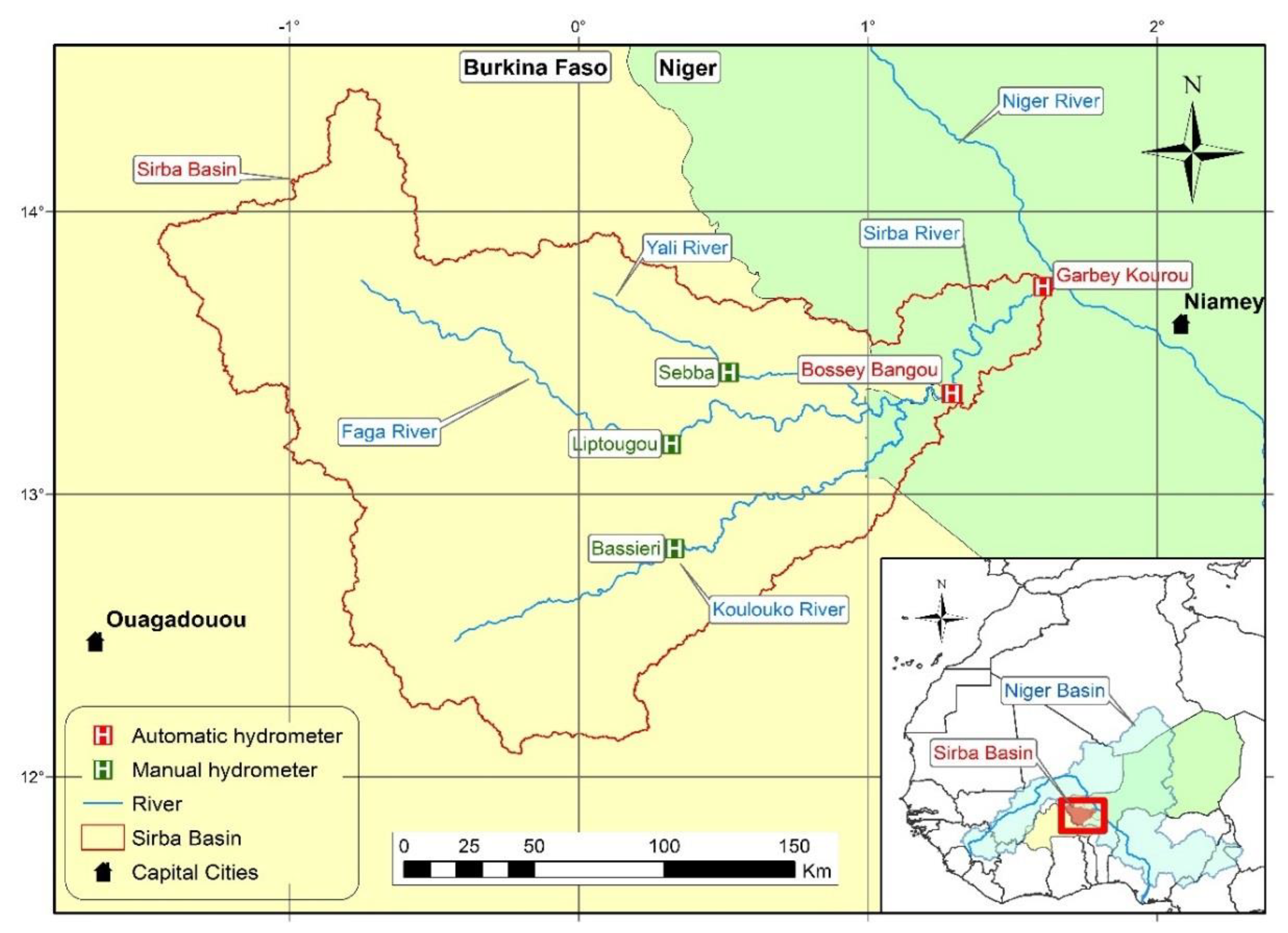
This study focused on the Sirba River, one of the major tributaries of the Middle Niger River. The basin covers 39,138 km2, most of which in Burkina Faso (93%), while the remaining part is in Niger (7%). The watershed is located in the Sahelian strip and is characterized by a wet season of approximately four months, from June to September [38,39]. The average streamflow, obtained from the Garbey Kourou hydrometer, shows that the hydrological behavior follows the rainfall pattern and that the Sirba River is an intermittent river, dry for approximately 200 days per year [30].
The Sirba River starts in Niger, downstream the confluence of Yali, Faga, and Koulouko rivers. The flow is measured by two automatic hydrometers in Niger (Bossey Bangou and Garbey Kourou) and by some manual hydrometers in Burkina Faso, among which the main ones are Sebba, Liptougou, and Bassieri (Figure 1).
2.2. The Hydrological Model
This work analyzed and attempted to improve the performances of Global Flood Awareness System (GloFAS), the global hydrological application operative in the study area. GloFAS is co-developed by the Joint Research Centre (JRC) of the European Commission and the European Centre for Medium-Range Weather Forecasts (ECMWF) and is based on the HTESSEL (Revised Tiled ECMWF Scheme for Surface Exchanges over Land) land-surface model and the Lisflood distributed hydrological model [31]. It is part of the Copernicus Emergency Management Service and uses the meteorological inputs of the ECMWF to provide probabilistic river discharge forecasts for up to 30 days.
The model parameters were assigned on a global regular grid of 0.1 × 0.1 degree (≈10 km), and the outputs were provided in a web platform for the whole globe with over 2000 reporting points providing detailed flood information worldwide, usually located around the main gauging stations (www.globalfloods.eu) [40]. GloFAS forecasts and products are freely accessible for everybody and for all use.
The model thus produced an ensemble of 51 forecasts that were used to evaluate the probabilities of thresholds exceedances [31,41]. There are five reporting points on the Sirba Basin: the Garbey Kourou point, active since the model implementation, and four other points located near the remaining hydrometers (Bossey Bangou, Sebba, Liptougou, and Bassieri) since May 2018. These reporting points were added after the request of the ANADIA 2.0 Project (Adaptation to climate change, disaster prevention, and agricultural development for food security) to increase the forecast density in this crucial area (Table 1).
There are two versions of the model: the original version (GloFAS 1.0), launched on 1 November 2011, that did not include calibration, and the updated one (GloFAS 2.0), launched on 14 November 2018, that was calibrated using the daily streamflow data from 1287 stations worldwide (including Garbey Kourou flow series). GloFAS 2.0 has improved the river discharge performance through an enhancement of routing scheme and groundwater model parameters forced by observed stream-flows and ECMWF reforecasts [32]. After the launch of the new version, GloFAS 1.0 was replaced by GloFAS 2.0 as the only operationally available hydrological model.
In November 2019, GloFAS was upgraded to version 2.1, whose model cycle included some smaller changes and introduced some new products. Importantly, the river discharge reanalysis and the related thresholds were updated using the officially released ERA5 (Atmospheric Reanalysis of ECMWF, fifth generation) [42]. This new model version was not considered in the study because the hydrological modelling was not changed and the differences between 2.0 and 2.1 were expected to be small and would not have changed the conclusions of the paper.
2.3. Materials
The materials used in this study consisted essentially of the Garbey Kourou flow time series, both observed and forecasted, and of the Sirba River hazard thresholds. The forecasted flow series contains two different datasets: (1) the GloFAS 1.0 series and (2) the GloFAS 2.0 series.
2.3.1. Observed Flow Series
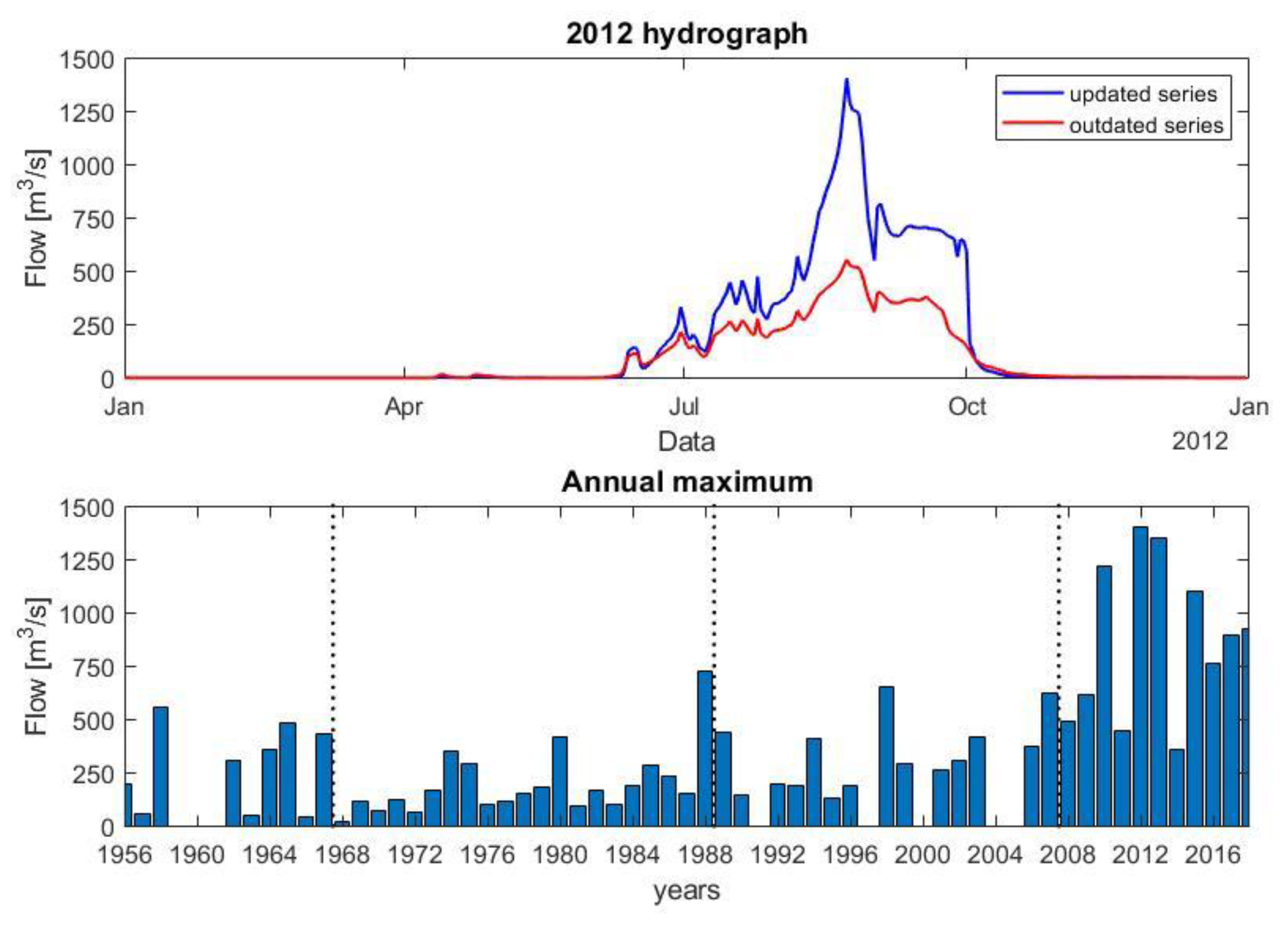
The historical discharge series contains the daily observations of the Garbey Kourou gauging station from 28 June 1956 to 31 December 2018. The flow series was subjected to a major revision in 2019 due to an outdated rating curve that was causing a substantial underestimation of the streamflow. The updated flow series fits much more of the river behavior (Figure 2). The hydrological analysis of the dataset highlighted three changepoints in 1968, 1989, and 2008, representing four climatic periods: (1) 1956–1967 wet period, (2) 1968–1988 great drought, (3) 1989–2007 rainfall and flow augmentation, and (4) 2008–present day flood period [30]. The flood period is characterized by the increase of the annual flow maxima and the flood-related damages [6]. Following the changepoints, the decision of considering only the river flow of the last period (2008–2018) was made.
2.3.2. Forecasted Flow Series
The GloFAS 1.0 dataset contains the forecasts from 1 April 2008 to 30 April 2018 for the Garbey Kourou reporting point. The daily forecasts were provided by GloFAS developers considering 3682 days of forecast runs, 30 forecast lead times, and 51 ensemble values in a 3682 × 31 × 51 matrix. The columns of the matrix represent the initial river discharge value and the 30 daily forecasts [31].
The GloFAS 2.0 dataset contains the forecasts from 1 January 1997 to 31 December 2018 for the Garbey Kourou reporting point. The forecasts were provided in three formats: with twice-weekly frequency and 11 ensemble values from 1 January 1997 to 31 December 2016, with twice-weekly frequency and 51 ensemble values from 1 January 2017 to 30 June 2017, and with daily frequency and 51 ensemble values from 1 July 2017 to 31 December 2018.
The datasets were used to perform two different types of analysis: (1) the evaluation of the improvements reached by the new version of GloFAS, and (2) the assessment of reliability for an application in an early warning system (EWS). These analyses were conducted between April 2008 and April 2018, in line with the changepoints and the flow series availability (Table 2).
2.3.3. Hazard Thresholds
The observed hazard thresholds were computed in conformity with the most advanced analysis techniques, considering the updated river hydrology and the related field effects. The annual maxima (Figure 2) of the historical discharge series showed a clear non-stationarity that was analyzed following not only the traditional generalized extreme value (GEV) approach but also the non-stationary (NS) GEV approach, which considers the hydrologic changes and the increase of the return time period in the last decades [23]. The thresholds were thus related to three indices: (1) the flow duration curve (FDC), obtained from the mean flow hydrology; (2) the stationary return time period based on the extreme analysis; and (3) the NS return period according to the hydrologic changes [27]. After the identification of thresholds and flood-prone areas, an inventory of the exposed items was made through a drone flight and a field survey [43]. Table 3 displays the thresholds, the indices, and the related field effects in the main riverine villages, underlining the importance of building an EWS [28].
The GloFAS hazard thresholds are the magnitudes of events with given return periods (2, 5, and 20 years), obtained from a climatological re-analysis based on Era-Interim (in GloFAS 1.0) and ERA5 (in GloFAS 2.0) [44,45]. The values in Table 4 highlight that the return periods were similar to those of the observed hazard thresholds, whereas the flow magnitudes were completely different (4 and 10 times lower). The magnitude differences are important for understanding the mismatch between observed and forecasted flow series. However, in probabilistic models such as GloFAS, the focus is on the warning given by the threshold exceeding rather than on the amount of the discharge.
2.4. Methods
The methods described in the following sections focus on the verification and optimization processes of the Sirba River forecasted discharges. The GloFAS outputs have been applied worldwide and verified several times, from Latin America to South and Southeast Asia [46,47,48]. These applications show that studies conducted on specific forecasting events (Brasil and Pakistan) consider all the ensemble values, although the evaluation of the quality of the model needs an unique deterministic value (Myanmar and Nepal) [49]. Moreover, applications for an EWS need a fixed forecast lead time and preferably a post-processing to improve the forecast quality (Perù) [50]. In this case, the data processing sorted each daily ensemble in ascending order and calculated the mean for the values from the 25th to the 75th percentile, allowing one value to be obtained, free of ensemble outliers, for every day of forecast.
The verification concerns the evaluation of forecast quality whereas the optimization is the process that reduces the discrepancy between observed and forecasted values. Continuous and categorical indices were used for the analysis. The optimization was developed from the user point of view by applying a set of correction factors to the model outputs. Therefore, the calibration was conducted on the model outputs instead of the internal model parameters [51,52,53,54,55]. All the analyses were conducted on 5 days forecasts, as established by the ANADIA 2.0 project, because of the time required to activate a strategic plan and secure the flood-prone areas [28]. The categorical indices were calculated on the yellow threshold exceeding (127 m3/s for GloFAS 1.0, 61 m3/s for GloFAS 2.0, and 600 m3/s for observed discharge and optimized models) in order to increase the sample size [27].
2.4.1. Forecast Verification
The forecast verification is based on fitting and reliability indices. The fitting verification between observed and forecasted values was realized through continuous indices. The streamflow was therefore considered as a continuous variable that can assume an infinite number of possible values, although both forecasts and observations are made using a finite number of discrete values [33]. For this purpose, the RMSE (root mean square error) observations standard deviation ratio (RSR) and the Nash–Sutcliffe efficiency (NSE) indices were used. The RSR detects the absolute systematic mean error of forecast after a penalization of large errors, whereas the NSE is a normalized statistic that determines the relative magnitude of the residual variance compared to the measured data variance [34,56,57].
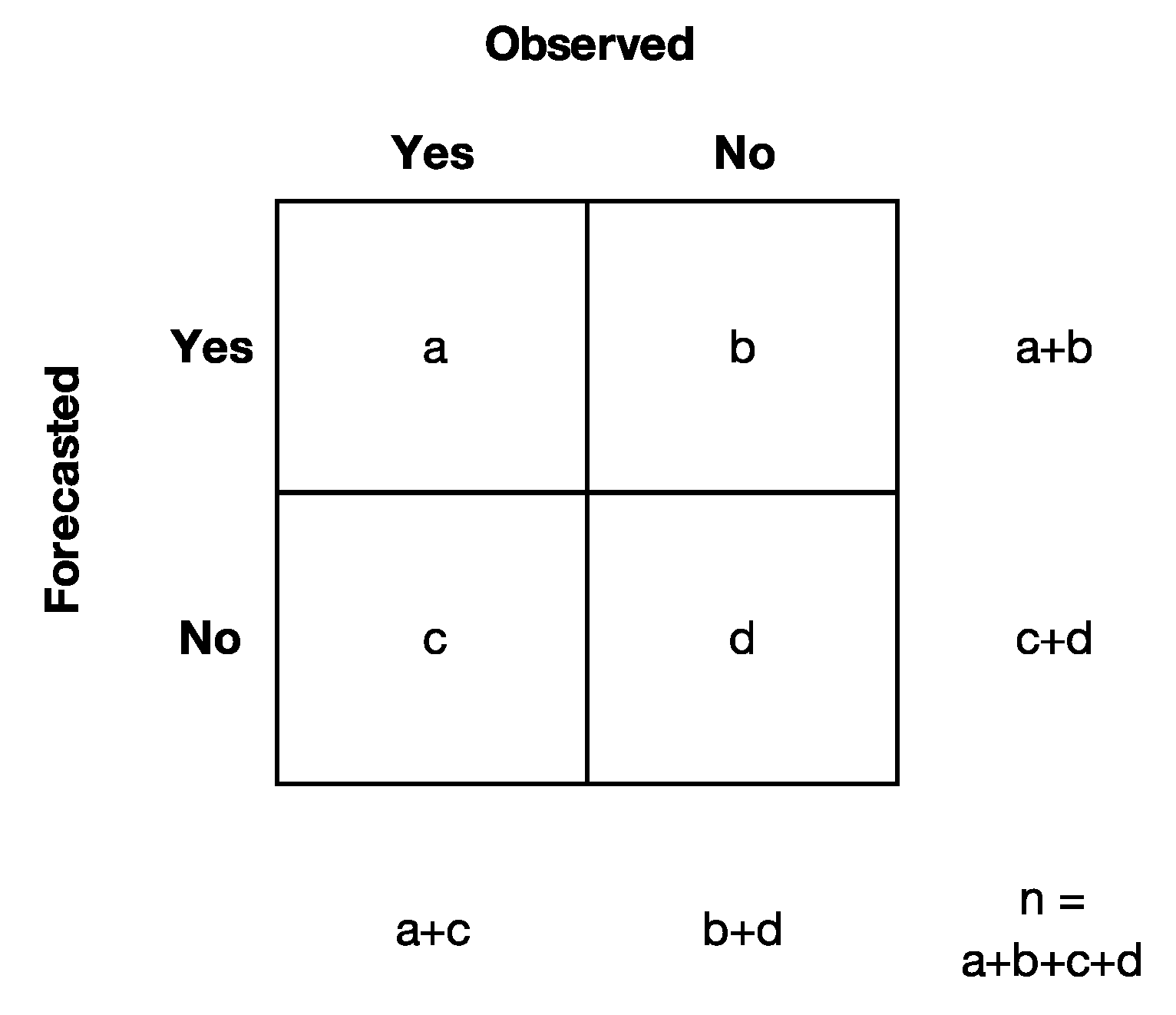
Then, in order to assess the reliability of forecasts in predicting flood events, the discharge was considered as a dichotomous variable of type “yes” or “no” referring to the specific “threshold exceeding” event. Hence, essentially, both forecasts and observations of this variable indicate the number of days in which the selected hazard threshold was exceeded (Figure 3).
The categorical indices calculated as reliability indicators are bias (BIAS), probability of detection (POD), false alarm rate (FAR), percent correct (PC), threat score (TS), and Heidke skill score (HSS) [31,33,34]. The objective of these indices is to detect the overall goodness of forecasts and completeness of information considering all the cases of detection (“hit”, “false alarm”, “miss”, “correct negatives”).
The accurate description and the formulation of the adopted continuous and categorical indices is reported in Appendix A.
2.4.2. Forecast Optimization
The optimization is the process that seeks to improve the reliability of forecasts. For this purpose, the flow time series were divided into two separate sub-datasets: a training period and a validation period. The training period is necessary to calculate the correction factors whereas the validation period is necessary to verify the performances of the new forecasts as modified by the correction factors. The dataset splitting was realized to ensure robustness both to the optimization and the verification procedures within the bounds of availability of the forecasts. The analysis datasets were thus divided into two equal periods of 5 years (training: 1 April 2008–31 December 2012, validation: 1 January 2013–31 December 2017), giving the same weight at training and validation [36,56].
Linear regression models were created to identify a relation, as much as possible, between forecasts and observations in the training datasets. The ordinary least squares (OLS) method was used to estimate the coefficients of the linear regression models [37]. The OLS objective is to find the linear function that minimizes the residual sum of squares (RSS), that is, the sum of the squares of the difference between the dependent variable values and those predicted under the linear regression model. The observed data were selected as response variable while the 5 days forecasts were selected as an explanatory variable. The training and validation datasets were divided into 12 homogeneous periods according to the river hydrology [30]. The discharges in the dry season (November to May) were grouped into a unique interval, the low-flow season (June and October) was considered with a monthly time-frame, whereas the medium- and high-flow season (July to September) was divided into periods of 10 days each (Table 5).
The relation between the two variables has been estimated as
where yt, xt, and et indicate the variable y, x, and e at time t; and f (…) and g (…) are any type of function. Equation (1) indicates the presence of serial correlation in the errors; this implies that the error et does not impact only on yt but also on the future realizations, yt+1, yt+2,…. The autocorrelation of the errors can be caused by the omission of an autocorrelated variable among the explanatory variables, or by the autocorrelated nature of the dependent variable, not sufficiently explained by x. Hence, with relation to Equation (1), a typical assumption of OLS is not, obviously, respected:
The OLS estimators are consequently no longer the best, but still linear and unbiased. Furthermore, the test statistics are no longer correct because the classic standard errors, on which they are based, tend to be underestimated. This problem was overcome by using the Newey–West heteroskedasticity and autocorrelation consistent (HAC) standard errors [57,58,59]. The use of OLS coefficient estimates in combination with HAC standard errors avoids specifying the exact nature of the error autocorrelation, necessary to construct an alternative estimator with minor variance. The possibility of non-normally distributed errors is ignored because it is not a necessary OLS assumption for achieving best linear unbiased estimator (BLUE), and the potential distortions in the calculation of the test statistics are already resolved by the HAC standard errors [60].
The functions chosen as f (…) in Equation (1) were polynomial functions of degrees 1, 2, 3, and 4. The OLS objective can also be understood as the maximization of R2; remembering that
This criterion was also used to choose the most suitable functional forms for the linear regression models. Hence, only OLS coefficient estimates significantly different from zero at the 0.05 level of linear regression models with highest R2 were chosen as correction factors of the forecasts. These factors were exclusively applied in the wet period (June to October) because the dry period was already correctly modelled.
In the following sections, in order to simplify the reading, various acronyms are used to indicate the four forecasted flow series: G1 (GloFAS 1.0), G2 (GloFAS 2.0), OG1 (optimized GloFAS 1.0), and OG2 (optimized GloFAS 2.0).
3. Results and Discussion
The results jointly considered the four forecasted series (5 days GloFAS 1.0 and 2.0 both in original and optimized format) and compared them with the observed flow series. The analysis timeframe covered the five years (2013–2017) of verification.
The preliminary analysis was conducted on the basic statistical parameters of maximum, minimum, and mean reached during the verification period (Table 6). The minima displayed that zero wa correctly forecasted by all models. Mean and maxima showed that the raw forecasts heavily underestimated the river discharge—the mean value was less than 1/10, whereas the maximum was less than 1/5 of the observed flow, in both versions of GloFAS. Moreover, G2 values were significantly lower than G1. After the optimization, mean values showed an over-forecasting in OG1 and an under-forecasting in OG2, although the maxima were both over-estimated (Table 6).
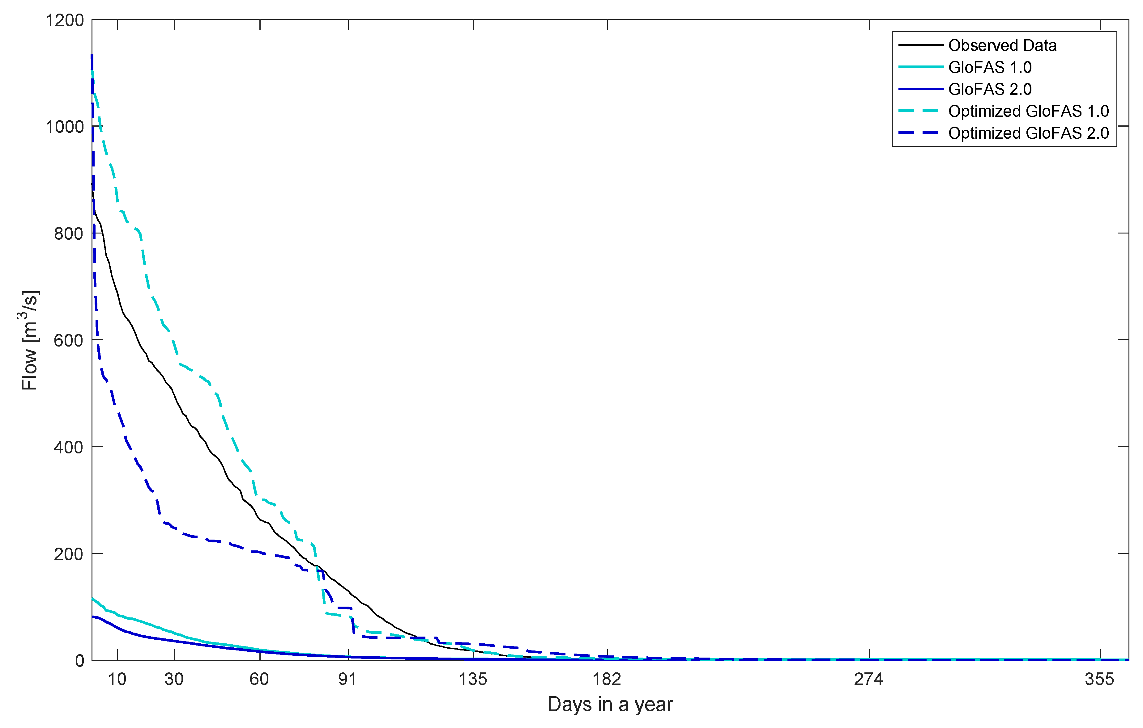
The flow duration curves confirmed the previous results, leading to some interesting observations: (1) G1 had serious problems in producing zero flow values (even for Q355); (2) the central part (Q60–Q135) was very similar between G1 and G2; (3) the highest values (Q1–Q10) were quite close in OG1, whereas in OG2 the Q1 is more than double the Q5; (4) in the interval Q5–Q80, the forecasts were over-forecasted in OG1 and under-forecasted in OG2; and (5) the behavior of OG1 and OG2 was the same from Q80 onwards, even if OG2 was higher than OG1 until Q200 and lower in the final part of the curve (Figure 4).
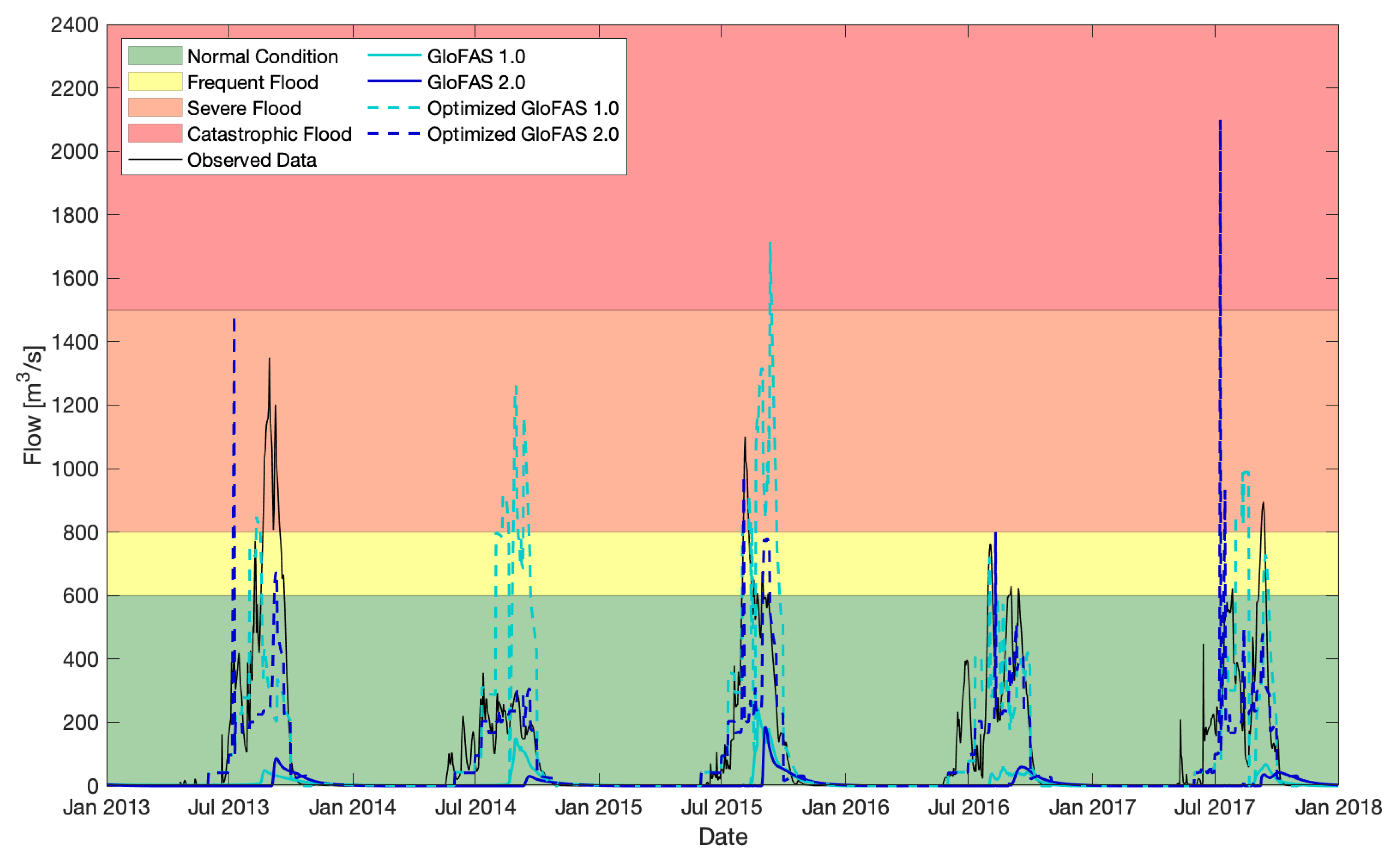
The hydrograph of observed and forecasted flows highlights the ability of all forecasts to capture the annual flow cycle, especially during the dry season (Figure 5). However, the wet season peaks were widely underestimated in the original versions, whereas the optimized forecasts tended to produce some outlier peaks. The outliers occurred every year, except for 2016 (OG2 in 2013 and 2017, and OG1 in 2014, 2015, and 2017).
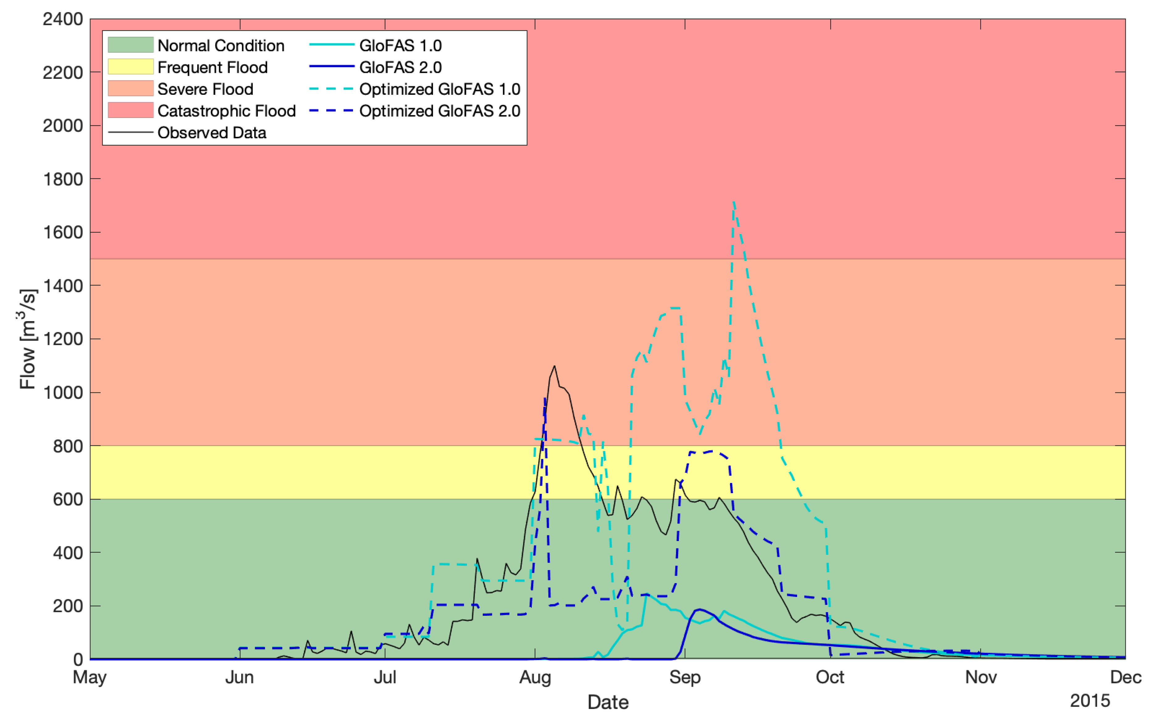
A single wet season is shown in Figure 6 in order to better describe the model behavior. The original models predicted values near zero for most of the time period. It is noticeable that in G2 the flow started at the end of August, whereas in G1 it began 15 days before. The optimized versions clearly showed an over-forecasting in OG1 and an under-forecasting in OG2. With regards to the peak values, observed flow and forecasts were quite different: (1) OG2 captured the start and the end of the highest flows (early August to mid-September), whereas OG1 identified the initial peak but overestimated the flow at the end of September; (2) the peaks were quite accurate in OG2, whereas OG1 over-forecasted them; (3) both optimized models properly identified the major peaks (early August and early September), but OG1 over-estimated the peak duration and OG2 under-estimated it.
The 2.0 version of GloFAS did not produce substantial improvements to the forecasts, according to RSR and NSE, and the overall quality even slightly deteriorated. However, some noteworthy enhancements could be reached with the optimization procedure (Table 7).
On the basis of performance ratings in Table 8, G1, G2, and OG1 showed unsatisfactory values, whereas the results obtained by OG2 were sufficiently satisfactory (RSR = 0.72 and NSE = 0.48) [34,61,62]. The optimization improved the performance of RSR (OG1 < G1 and OG2 < G2) and NSE (OG1 > G1 and OG2 > G2) for both model versions. However, it is interesting to note that OG2 performed better than OG1, although G2 achieved worse results than G1 for both RSR and NSE. Therefore, the improvement was significant only for OG2.
The categorical indices displayed different results (Table 9). BIAS values underlined the under-forecasting or the over-forecasting in terms of threshold exceeding. Therefore, G1, G2, and OG2 under-forecast the yes events, whereas OG1 showed an over-forecasting. The BIAS values exhibited a redundancy (OG1) and a deficiency (G1, G2, and OG2), which suggest that the FAR for OG1, and the POD for G1, G2, and OG2 would not be particularly satisfying. POD and FAR are the fundamental parameters that are analyzed for an EWS application. The best POD performance belonged to OG1, whereas the best FAR performance belonged to G2. However, these values were quite unsatisfactory for all the models because FAR ≥ 60% and POD ≤ 33% were slightly insufficient in activating an EWS mechanism. PC was influenced by the “correct negatives” rather than by the “hits” due to the high amount of values under the yellow threshold. The percentage of “correct negatives” decreased in the optimized models. Therefore, the under-forecasted OG2 appeared to be more accurate than OG1. The quality of forecast in predicting threshold exceeding was assessed by TS. This index considered both “hits” and “false alarms”, thus incorporating the POD and FAR features. It demonstrated that, giving the same weight to POD and FAR, G2 and OG1 were slightly better than G1 and OG2 for an EWS application. TS confirmed the non-optimal behavior observed in POD and FAR and quantified that only 13% (G2 and OG1) and 5–8% (G1 and OG2) of threshold exceeding were correctly identified. HSS considers both the success ratio (1-FAR) and the number of correct random chance forecasts. This skill index is generally used to evaluate rare events [63]. The best results, such as TS, were reached by G2 (0.21) and OG1 (0.18).
The analyses demonstrated that the GloFAS 1.0 system badly forecasted the flow in the Sahelian area as declared by Alfieri et al. in 2013 [31]. The Sahelian discharge forecasting complexity is related both to a non-homogeneous watershed response and to several difficulties in correctly predicting the meteorological forcing [35,51,64]. The calibration conducted by Hirpa et al. in 2018 [32] for GloFAS 2.0 contributed to the improvement of the forecast behavior in terms of categorical indices. On the contrary, the continuous indices were not improved because the calibration was realized before the revision of the Garbey Kourou historical discharge series by using an outdated and unreliable series [30]. The optimization allowed for the alignment of the forecasted hydrograph shape to the observed flow, even though the flow magnitude was still underestimated.
The continuous indices showed that (1) G1 and G2 are flow predictors less precise than the mean flow, (2) OG1 insufficiently improved the quality of the model, and (3) OG2 obtained results fairly satisfactory according to the classification of Moriasi et al. in 2007 [34]. Although the performances of forecasts were lower than the literature values for the continuous indices, OG2 proved to be the best solution to forecast the river flow [34,46,50]. The categorical indices demonstrated the over-forecasting of OG1 and the under-forecasting of OG2. Thus, both original and optimized models showed a poor reliability in predicting flood events in the Sirba River Basin. The high number of “false alarms” and the low number of “hits” do not allow for people to be alerted. The forecasts correctly identifying the threshold exceeding were indeed about 10% (13% G2 and OG1, and 5–8% G1 and OG2). Therefore, OG2 can be used to predict the hydrological evolution but not to activate the alert mechanisms.
The analyses underlined the fundamental role of the hazard thresholds—the GloFAS thresholds were less than 1/3 (G1) and 1/10 (G2) of the observed and field-calibrated thresholds [27,28]. The categorical indices showed that coincidental events were possible and quite common, although the flow thresholds were completely different. However, it is very important to consider the GloFAS warnings instead of the actual forecasted flow. The Sirba case of study demonstrated that even the maximum forecasted flow did not cause any damage to the riverine communities because it was an ordinary discharge that is overpassed 90 days every year.
4. Conclusions
The Sahelian hydrological behavior has totally changed in the last decades, generating a high number of floods characterized by unprecedented magnitudes. The change has been caused by the increase of extreme rainfall events coupled with land use changes that generated the rupture of the endoreic basin and the growth of the secondary river network. The Sirba River, one of the major tributaries of Niger River, has been particularly touched by this phenomenon. Flood-related losses have pushed the national departments and the scientific community to develop an early warning system.
Previous studies have already analyzed the hydrology. The joint use of the hydraulic model with the hydrometric observations allows for exposed villages to be alerted a day earlier thanks to hydrometric observations. Therefore, the aim of this research was to evaluate the application of GloFAS (Global Flood Awareness System) in the Sirba River in order to predict the arrival of high flows a few days in advance. The study was conducted on two GloFAS systems: the original GloFAS 1.0 and the newest 2.0 version. The analysis evaluated and optimized the re-forecasts of a 10 year period (2008–2017). The 5 days forecasts were chosen in order to have adequate time to activate the field adaptive measures. The optimization was conducted from the user point of view by correcting the model outputs instead of the model parameters. The datasets were split into 5 years for training and 5 years for validation. The computation of the correction factors was performed through linear regression between observed and forecasted flow. The validation considered continuous and categorical indices.
The results showed the poor reliability of both version 1.0 and 2.0 for the original forecasts. These forecasts, as flow predictors, were less accurate than the mean flow. Although the calibration for version 2.0 conducted by GloFAS developers improved the EWS skills, the flow deficit increased because the calibration was based on an outdated and unreliable flow series of the Garbey Kourou hydrometer. The optimization procedures produced a substantial improvement in forecast accuracy. The continuous indices of optimized GloFAS 2.0 were quite satisfactory with regard to flow prediction, whereas the improvements were not conspicuous in the 1.0 optimized model. Therefore, the enhancement of GloFAS 2.0 demonstrated the importance of the optimization in regulating the shape of the forecasted hydrograph rather than in adjusting its intensity. The reliability of the flow peak forecasts, measured by the categorical indices, was low for both the original and optimized models, as the percentage of correctly predicted floods was approximately 10%. The results also illustrated the level of hazard threshold on which to develop a hydrological model in order to correctly quantify the river discharges and to not only issue warnings. This outcome could be used for a new version of the GloFAS system.
However, the optimized GloFAS 2.0 will be used in the EWS platform for the Sirba River. This application will be useful in providing reliable information on the evolution of river hydrology, but less appropriate to send alerts to the exposed populations. In order to guarantee the reliability of the EWS platform, the alerts will only be sent using the in situ measurements.
Future work will involve an enhanced collaboration with hydrological model developers and the implementation of the Sirba EWS platform with the new updated versions of GloFAS. Model calibration on the observed flow series or the utilization of a regional hydrological model could improve peak forecasting. These studies will allow the use of hydrological models for the EWS, which is currently conducted with in situ observations only.
Author Contributions
G.P.: methodology, analysis and elaboration of data, writing—original draft; G.M.: methodology, data collection, analysis and elaboration of data, writing—original draft; A.P.: methodology, supervision, validation, writing—review and editing; V.B.: supervision, validation, writing—review and editing; E.Z.: supervision, forecast production, validation, writing—review and editing; M.R.: methodology, supervision, validation, writing—review and editing. All authors have read and agreed to the published version of the manuscript.
Funding
This research was funded by the ANADIA 2.0 Project (Adaptation to climate change, disaster prevention and agricultural development for food security) by the Italian Agency for Development Cooperation, the Institute of Bioeconomy of the National Research Council of Italy (IBE-CNR), the Interuniversity Department of Regional and Urban Studies and Planning of the Polytechnic and University of Turin (DIST-POLITO), the National Directorate for Meteorology of Niger (DMN), and the Directorate for Hydrology of Niger (DH).
Acknowledgments
The authors would like to thank the Italian Agency for Development Cooperation for supporting the ANADIA 2.0 Project and the actions that allowed the development of this assessment. We would like to express our deepest gratitude to Mohamed Housseini Ibrahim (Directorate for Hydrology of Niger) for the historical flow series and to Alessandro Toffoli (University of Melbourne) for critical review of the manuscript.
Conflicts of Interest
The authors declare no conflict of interest. The funders had no role in the design of the study; in the collection, analyses, or interpretation of data; in the writing of the manuscript; or in the decision to publish the results.
Appendix A
Appendix A.1. Continuous Indices
The RMSE observation standard deviation ratio (RSR) is the root mean square error standardized using the standard deviation of the observations.
where T is number of observed/forecasted days, F is forecasts, and O is observed data.
RSR varies from the optimal value of 0 to +∞. Values ≤ 0.7 are considered satisfactory, whereas values > 1 indicate that the model forecasts are a worse predictor than the observed mean flow.
The Nash–Sutcliffe efficiency (NSE) was introduced specifically to evaluate the accuracy of hydrological model forecasts. It is a normalized statistic that determines the relative magnitude of the residual variance, “noise”, compared to the measured data variance, “information”:
NSE ranges between −∞ and the optimal value of 1 and, for RSR, large errors are penalized. Because a perfect score is impossible to achieve in practice, the literature suggests that the forecasts can be considered satisfactory with values ≥ 0.5. Instead, values ≤ 0 indicate that the observed mean flow is a better predictor than the model forecasts.
Appendix A.2. Categorical Indices
Bias represents the sum of the forecasted yes events divided by the sum of observed yes events:
A perfect score for BIAS is equal to 1. This value implies that there are the same number of forecasted and observed yes events. Values > 1 indicate over-forecasting, and BIAS < 1 under-forecasting.
The probability of detection represents the sum of the correctly forecasted yes events divided by the sum of observed yes events:
The best possible POD result is 1. Because it ignores the “false alarms”, it can be artificially improved by issuing more forecasted yes events in order to increase the number of “hits”. An evaluation of POD without considering other indices can be therefore misleading.
The false alarm rate represents the sum of the “false alarms” divided by the sum of the forecasted yes events:
The best FAR result is 0. Because it ignores the “misses”, it is not an index that can be evaluated by itself. Therefore, it is usually examined with the POD, as explained above.
The percent correct represents the sum of correctly forecasted, both yes and no, events divided by the number of total events:
PC is expressed as a percentage, where 0 is the worst result and 100 the best. Because it considers both the “hits” and the “correct negatives” it provides an evaluation of the overall goodness of forecasts. If the observed no events are much more than the yes events it can lead to overrating the forecast reliability.
The threat score (TS) represents the sum of the correctly forecasted yes events divided by the sum of “hits”, “false alarms”, and “misses”:
The best value for the TS is equal to 1. It penalizes equally both the “false alarms” and the “misses”. Because the “correct negatives” are not considered in the calculation, it is a reliable index for a dataset in which observed yes events are rare or uncommon.
The following index is a skill score. The Heidke skill score (HSS) is a generalized skill score, based on the percent correct, where the standard control forecasts are random forecasts statistically independent from the observations:
Perfect forecasts have an HSS equal to 1, whereas forecasts have no skill when HSS is ≤ 0. HSS measures the fraction of the correctly forecasted, both yes and no, events after eliminating the forecasted events that are correct due purely to random chance.
References
- EMDAT. The Emergency Events Database. Available online: https://www.emdat.be/ (accessed on 18 September 2019).
- Berghuijs, W.R.; Aalbers, E.E.; Larsen, J.R.; Trancoso, R.; Woods, R.A. Recent changes in extreme floods across multiple continents. Environ. Res. Lett. 2017, 12, 114035. [Google Scholar] [CrossRef]
- Nka, B.N.; Oudin, L.; Karambiri, H.; Paturel, J.E.; Ribstein, P. Trends in floods in West Africa: Analysis based on 11 catchments in the region. Hydrol. Earth Syst. Sci. 2015, 19, 4707–4719. [Google Scholar] [CrossRef] [Green Version]
- Descroix, L.; Genthon, P.; Amogu, O.; Rajot, J.L.; Sighomnou, D.; Vauclin, M. Change in Sahelian Rivers hydrograph: The case of recent red floods of the Niger River in the Niamey region. Glob. Planet. Chang. 2012, 98–99, 18–30. [Google Scholar] [CrossRef]
- Panthou, G.; Vischel, T.; Lebel, T.; Quantin, G.; Pugin, A.-C.F.; Blanchet, J.; Ali, A. From pointwise testing to a regional vision: An integrated statistical approach to detect nonstationarity in extreme daily rainfall. Application to the Sahelian region: Regional Extreme Rainfall Stationarity. J. Geophys. Res. Atmos. 2013, 118, 8222–8237. [Google Scholar] [CrossRef]
- Fiorillo, E.; Crisci, A.; Issa, H.; Maracchi, G.; Morabito, M.; Tarchiani, V. Recent changes of floods and related impacts in Niger based on the ANADIA Niger flood database. Climate 2018, 6, 59. [Google Scholar] [CrossRef] [Green Version]
- Roudier, P.; Ducharne, A.; Feyen, L. Climate change impacts on runoff in West Africa: A review. Hydrol. Earth Syst. Sci. 2014, 18, 2789–2801. [Google Scholar] [CrossRef] [Green Version]
- Seidou, O. Climate change may result in more water availability in parts of the African Sahel. In Innovations and Interdisciplinary Solutions for Underserved Areas; Kebe, C.M.F., Gueye, A., Ndiaye, A., Garba, A., Eds.; Springer International Publishing: Cham, Switzerland, 2018; Volume 249, pp. 143–152. ISBN 978-3-319-98877-1. [Google Scholar]
- Amogu, O.; Descroix, L.; Yéro, K.S.; Le Breton, E.; Mamadou, I.; Ali, A.; Vischel, T.; Bader, J.-C.; Moussa, I.B.; Gautier, E.; et al. Increasing river flows in the Sahel? Water 2010, 2, 170–199. [Google Scholar] [CrossRef] [Green Version]
- Descroix, L.; Mahé, G.; Lebel, T.; Favreau, G.; Galle, S.; Gautier, E.; Olivry, J.C.; Albergel, J.; Amogu, O.; Cappelaere, B.; et al. Spatio-Temporal variability of hydrological regimes around the boundaries between Sahelian and Sudanian areas of West Africa: A synthesis. J. Hydrol. 2009, 375, 90–102. [Google Scholar] [CrossRef]
- Aich, V.; Koné, B.; Hattermann, F.F.; Müller, E.N. Floods in the Niger basin—Analysis and attribution. Nat. Hazards Earth Syst. Sci. Discuss. 2014, 2, 5171–5212. [Google Scholar] [CrossRef]
- Aich, V.; Liersch, S.; Vetter, T.; Andersson, J.C.M.; Müller, E.N.; Hattermann, F.F. Climate or land use?—Attribution of changes in river flooding in the Sahel zone. Water 2015, 7, 2796–2820. [Google Scholar]
- Sighomnou, D.; Descroix, L.; Genthon, P.; Mahé, G.; Moussa, I.B.; Gautier, E.; Mamadou, I.; Vandervaere, J.P.; Bachir, T.; Coulibaly, B.; et al. La crue de 2012 à Niamey: Un paroxysme du paradoxe du Sahel? Sci. Chang. Planetaires Secher. 2013, 24, 3–13. [Google Scholar]
- Fiorillo, E.; Maselli, F.; Tarchiani, V.; Vignaroli, P. Analysis of land degradation processes on a tiger bush plateau in South West Niger using MODIS and LANDSAT TM/ETM+ data. Int. J. Appl. Earth Obs. Geoinf. 2017, 62, 56–68. [Google Scholar] [CrossRef]
- Leblanc, M.J.; Favreau, G.; Massuel, S.; Tweed, S.O.; Loireau, M.; Cappelaere, B. Land clearance and hydrological change in the Sahel: SW Niger. Glob. Planet. Chang. 2008, 61, 135–150. [Google Scholar] [CrossRef]
- Amogu, O.; Esteves, M.; Vandervaere, J.-P.; Malam Abdou, M.; Panthou, G.; Rajot, J.-L.; Souley Yéro, K.; Boubkraoui, S.; Lapetite, J.-M.; Dessay, N.; et al. Runoff evolution due to land-use change in a small Sahelian catchment. Hydrol. Sci. J. 2015, 60, 78–95. [Google Scholar] [CrossRef]
- Descroix, L.; Guichard, F.; Grippa, M.; Lambert, L.; Panthou, G.; Mahé, G.; Gal, L.; Dardel, C.; Quantin, G.; Kergoat, L.; et al. Evolution of surface hydrology in the Sahelo-Sudanian strip: An updated review. Water 2018, 10, 748. [Google Scholar] [CrossRef] [Green Version]
- Descroix, L. Processus et Enjeux D’eau en Afrique de l’Ouest Soudano-Sahélienne; Editions des Archives Contemporaines: Paris, France, 2018; ISBN 978-2-8130-0314-0. [Google Scholar]
- Mamadou, I.; Gautier, E.; Descroix, L.; Noma, I.; Bouzou Moussa, I.; Faran Maiga, O.; Genthon, P.; Amogu, O.; Malam Abdou, M.; Vandervaere, J.P. Exorheism growth as an explanation of increasing flooding in the Sahel. Catena 2015, 131, 130–139. [Google Scholar] [CrossRef]
- Housseini Ibrahim, M. Note sur la Situation Hydrologique du Fleuve Niger a Niamey—Alerte Rouge a Niamey au 31 Août 2019; Autorite du Bassin du Niger (NBA): Niamey, Niger, 2019. [Google Scholar]
- Mostert, E.; Junier, S.J. The European flood risk directive: Challenges for research. Hydrol. Earth Syst. Sci. Discuss. 2009, 6, 4961–4988. [Google Scholar] [CrossRef]
- Smith, R. Directive 2008/94/EC of the European Parliament and of the Council of 22 October 2008; European Parliament: Brussels, Belgium; European Council: Brussels, Belgium, 2007; pp. 423–426. [Google Scholar]
- Wilcox, C.; Vischel, T.; Panthou, G.; Bodian, A.; Blanchet, J.; Descroix, L.; Quantin, G.; Cassé, C.; Tanimoun, B.; Kone, S. Trends in hydrological extremes in the Senegal and Niger Rivers. J. Hydrol. 2018, 566, 531–545. [Google Scholar] [CrossRef]
- Zschau, J.; Küppers, A.N. Early Warning Systems for Natural Disaster Reduction, 1st ed.; Spriger: New York, NY, USA, 2003; ISBN 978-3-642-55903-7. [Google Scholar]
- Basha, E.; Rus, D. Design of early warning flood detection systems for developing countries. In Proceedings of the IEEE 2007 International Conference on Information and Communication Technologies and Development, Bangalore, India, 15–16 December 2007; pp. 1–10. [Google Scholar]
- Gautam, D.K.; Phaiju, A.G. Community based approach to flood early warning in west Rapti River Basin of Nepal. J. Integr. Disaster Risk Manag. 2013, 15. [Google Scholar] [CrossRef]
- Massazza, G.; Tamagnone, P.; Wilcox, C.; Belcore, E.; Pezzoli, A.; Vischel, T.; Panthou, G.; Housseini Ibrahim, M.; Tiepolo, M.; Tarchiani, V.; et al. Flood hazard scenarios of the Sirba river (Niger): Evaluation of the hazard thresholds and flooding areas. Water 2019, 11, 1018. [Google Scholar] [CrossRef] [Green Version]
- Tiepolo, M.; Rosso, M.; Massazza, G.; Belcore, E.; Issa, S.; Braccio, S. Flood assessment for risk-informed planning along the Sirba river, Niger. Sustainability 2019, 11, 4003. [Google Scholar] [CrossRef] [Green Version]
- Krzhizhanovskaya, V.V.; Shirshov, G.S.; Melnikova, N.B.; Belleman, R.G.; Rusadi, F.I.; Broekhuijsen, B.J.; Gouldby, B.P.; Lhomme, J.; Balis, B.; Bubak, M.; et al. Flood early warning system: Design, implementation and computational modules. Procedia Comput. Sci. 2011, 4, 106–115. [Google Scholar] [CrossRef] [Green Version]
- Tamagnone, P.; Massazza, G.; Pezzoli, A.; Rosso, M. Hydrology of the Sirba river: Updating and analysis of discharge time series. Water 2019, 11, 156. [Google Scholar] [CrossRef] [Green Version]
- Alfieri, L.; Burek, P.; Dutra, E.; Krzeminski, B.; Muraro, D.; Thielen, J.; Pappenberger, F. GloFAS—Global ensemble streamflow forecasting and flood early warning. Hydrol. Earth Syst. Sci. Discuss. 2013, 9, 12293–12332. [Google Scholar] [CrossRef]
- Hirpa, F.A.; Salamon, P.; Beck, H.E.; Lorini, V.; Alfieri, L.; Zsoter, E.; Dadson, S.J. Calibration of the Global Flood Awareness System (GloFAS) using daily streamflow data. J. Hydrol. 2018, 566, 595–606. [Google Scholar] [CrossRef]
- Wilks, D.S. Statistical methods in the atmospheric sciences. In International Geophysics Series, 2nd ed.; Academic Press: Cambridge, MA, USA, 2006; ISBN 978-0-12-751966-1. [Google Scholar]
- Moriasi, D.N.; Arnold, J.G.; Van Liew, M.W.; Bingner, R.L.; Harmel, R.D.; Veith, T.L. Model evaluation guidelines for systematic quantification of accuracy in watershed simulations. Trans. ASABE 2007, 50, 885–900. [Google Scholar] [CrossRef]
- Ali, A.; Amani, A.; Diedhiou, A.; Lebel, T. Rainfall estimation in the Sahel. Part II: Evaluation of rain gauge networks in the CILSS countries and objective intercomparison of rainfall products. J. Appl. Meteorol. 2005, 44, 1707–1722. [Google Scholar] [CrossRef]
- ASCE Task Committee on Application of Artificial Neural Networks in Hydrology. Artificial Neural Networks in Hydrology. II: Hydrologic applications. J. Hydrol. Eng. 2000, 5, 124–137. [Google Scholar] [CrossRef]
- Kutner, M.H. Applied Linear Statistical Models; McGraw-Hill International Edition; McGraw-Hill Irwin: New York, NY, USA, 2005; ISBN 978-0-07-112221-4. [Google Scholar]
- Bigi, V.; Pezzoli, A.; Rosso, M. Past and future precipitation trend analysis for the City of Niamey (Niger): An overview. Climate 2018, 6, 73. [Google Scholar] [CrossRef] [Green Version]
- Tiepolo, M.; Tarchiani, V. Risque et Adaptation Climatique Dans la Région Tillabéri, Niger; L’Harmattan: Paris, France, 2016; ISBN 978-2-343-08493-0. [Google Scholar]
- GloFAS (Global Flood Awareness System). Available online: http://www.globalfloods.eu/ (accessed on 4 September 2019).
- Zajac, Z.; Revilla-Romero, B.; Salamon, P.; Burek, P.; Hirpa, F.A.; Beck, H. The impact of lake and reservoir parameterization on global streamflow simulation. J. Hydrol. 2017, 548, 552–568. [Google Scholar] [CrossRef]
- Harrigan, S.; Zsoter, E.; Alfieri, L.; Prudhomme, C.; Salamon, P.; Wetterhall, F.; Barnard, C.; Cloke, H.; Pappenberger, F. GloFAS-ERA5 operational global river discharge reanalysis 1979–present. Hydrol. Soil Sci. Hydrol. 2020. [Google Scholar] [CrossRef] [Green Version]
- Belcore, E.; Piras, M.; Pezzoli, A.; Massazza, G.; Rosso, M. Raspberry PI 3 multispectral low-cost sensor for UAV based remote sensing. Case study in South-West Niger. ISPRS Int. Arch. Photogramm. Remote Sens. Spat. Inf. Sci. 2019, 207–214. [Google Scholar] [CrossRef] [Green Version]
- Hirpa, F.A.; Salamon, P.; Alfieri, L.; Pozo, J.T.; Zsoter, E.; Pappenberger, F. The effect of reference climatology on global flood forecasting. J. Hydrometeorol. 2016, 17, 1131–1145. [Google Scholar] [CrossRef] [Green Version]
- Alfieri, L.; Zsoter, E.; Harrigan, S.; Aga Hirpa, F.; Lavaysse, C.; Prudhomme, C.; Salamon, P. Range-Dependent thresholds for global flood early warning. J. Hydrol. X 2019, 4, 100034. [Google Scholar] [CrossRef]
- GloFAS. Case Study: Myanmar and Nepal. Available online: http://www.globalfloods.eu/get-involved/case-study-myanmar-nepal/ (accessed on 17 September 2019).
- Case Study—2010 Pakistan Floods. Available online: http://www.globalfloods.eu/get-involved/case-study-2010-pakistan-floods/ (accessed on 17 September 2019).
- Moraes, M. GloFAS as a Flood Alert System in Acre Civil Defense; National Center for Monitoring and Early Warning for Natural Disaster: Sao Paulo, Brazil, 2018. [Google Scholar]
- Gilleland, E.; Pappenberger, F.; Brown, B.; Ebert, E.; Richardson, D. Verification of meteorological forecasts for hydrological applications. In Handbook of Hydrometeorological Ensemble Forecasting; Duan, Q., Pappenberger, F., Wood, A., Cloke, H.L., Schaake, J.C., Eds.; Springer: Berlin/Heidelberg, Germany, 2019; pp. 923–951. ISBN 978-3-642-39925-1. [Google Scholar]
- Bischiniotis, K.; van den Hurk, B.; Zsoter, E.; Coughlan de Perez, E.; Grillakis, M.; Aerts, J.C.J.H. Evaluation of a global ensemble flood prediction system in Peru. Hydrol. Sci. J. 2019, 64, 1171–1189. [Google Scholar] [CrossRef] [Green Version]
- Andersson, J.C.M.; Ali, A.; Arheimer, B.; Gustafsson, D.; Minoungou, B. Providing peak river flow statistics and forecasting in the Niger River basin. Phys. Chem. Earth Parts A B C 2017, 100, 3–12. [Google Scholar] [CrossRef]
- Andersson, J.C.M.; Arheimer, B.; Traoré, F.; Gustafsson, D.; Ali, A. Process refinements improve a hydrological model concept applied to the Niger River basin. Hydrol. Process. 2017, 31, 4540–4554. [Google Scholar] [CrossRef] [Green Version]
- Huo, J.; Liu, L.; Zhang, Y. An improved multi-cores parallel artificial Bee colony optimization algorithm for parameters calibration of hydrological model. Future Gener. Comput. Syst. 2018, 81, 492–504. [Google Scholar] [CrossRef]
- Jiang, Y.; Li, X.; Huang, C. Automatic calibration a hydrological model using a master-slave swarms shuffling evolution algorithm based on self-adaptive particle swarm optimization. Expert Syst. Appl. 2013, 40, 752–757. [Google Scholar] [CrossRef]
- Wang, Y.; Brubaker, K. Multi-Objective model auto-calibration and reduced parameterization: Exploiting gradient-based optimization tool for a hydrologic model. Environ. Model. Softw. 2015, 70, 1–15. [Google Scholar] [CrossRef]
- Hsu, K.; Gupta, H.V.; Sorooshian, S. Artificial neural network modeling of the rainfall-runoff process. Water Resour. Res. 1995, 31, 2517–2530. [Google Scholar] [CrossRef]
- Andrews, D.W.K. Heteroskedasticity and autocorrelation consistent covariance matrix estimation. Econometrica 1991, 59, 817. [Google Scholar] [CrossRef]
- Andrews, D.W.K.; Monahan, J.C. An Improved heteroskedasticity and autocorrelation consistent covariance matrix estimator. Econometrica 1992, 60, 953. [Google Scholar] [CrossRef]
- Newey, W.K.; West, K.D. A simple, positive semi-definite, heteroskedasticity and autocorrelation consistent covariance matrix. Econometrica 1987, 55, 703. [Google Scholar] [CrossRef]
- Hill, R.C.; Griffiths, W.E.; Lim, G.C. Principles of Econometrics, 4th ed.; Wiley: Hoboken, NJ, USA, 2011; ISBN 978-0-470-62673-3. [Google Scholar]
- Ritter, A.; Muñoz-Carpena, R. Performance evaluation of hydrological models: Statistical significance for reducing subjectivity in goodness-of-fit assessments. J. Hydrol. 2013, 480, 33–45. [Google Scholar] [CrossRef]
- Gassman, P.W.; Reyes, M.R.; Green, C.H.; Arnold, J.G. The soil and water assessment tool: Historical development, applications, and future research directions. Trans. ASABE 2007, 50, 1211–1250. [Google Scholar] [CrossRef] [Green Version]
- Doswell, C.A.; Da Vies-Jones, R.; Keller, D.L. On summary measure of skill in rare event forecatsing based on contingency tables. Weather Forecast. 1990, 5, 576–585. [Google Scholar] [CrossRef] [Green Version]
- Arheimer, B.; Pimentel, R.; Isberg, K.; Crochemore, L.; Andersson, J.C.M.; Hasan, A.; Pineda, L. Global catchment modelling using World-Wide HYPE (WWH), open data, and stepwise parameter estimation. Hydrol. Earth Syst. Sci. 2020, 24, 535–559. [Google Scholar] [CrossRef] [Green Version]
Figure 1.
Geographical framework of the study area: the Sirba River Basin with the hydrometric gauging stations, the main hydrographic network, and the administrative boundaries. Bottom right: West Africa overview.
Figure 1.
Geographical framework of the study area: the Sirba River Basin with the hydrometric gauging stations, the main hydrographic network, and the administrative boundaries. Bottom right: West Africa overview.

Figure 2.
Historical discharge series of Garbey Kourou gauging station [30]. Top: hydrograph observed in 2012 with the outdated and the updated (ANADIA) approach; bottom: annual maxima of the discharge and the three changepoints (1968, 1989, and 2008).
Figure 2.
Historical discharge series of Garbey Kourou gauging station [30]. Top: hydrograph observed in 2012 with the outdated and the updated (ANADIA) approach; bottom: annual maxima of the discharge and the three changepoints (1968, 1989, and 2008).

Figure 3.
Contingency table used to calculate the categorical indices. Each letter indicates the number of times the specific event occurs: a = “hits”, b = “false alarms”, c = “misses”, d = “correct negatives”.
Figure 3.
Contingency table used to calculate the categorical indices. Each letter indicates the number of times the specific event occurs: a = “hits”, b = “false alarms”, c = “misses”, d = “correct negatives”.

Figure 4.
Flow duration curve of the Sirba River at Garbey Kourou in the verification years 2013–2017. Observed flow, and 1.0 and 2.0 (5 days) GloFAS forecasts before and after the optimization.
Figure 4.
Flow duration curve of the Sirba River at Garbey Kourou in the verification years 2013–2017. Observed flow, and 1.0 and 2.0 (5 days) GloFAS forecasts before and after the optimization.

Figure 5.
Hydrograph of the Sirba River at Garbey Kourou in the verification years 2013–2017. Observed flow, and 1.0 and 2.0 (5 days) GloFAS forecasts before and after the optimization.
Figure 5.
Hydrograph of the Sirba River at Garbey Kourou in the verification years 2013–2017. Observed flow, and 1.0 and 2.0 (5 days) GloFAS forecasts before and after the optimization.

Figure 6.
Hydrograph of the Sirba River at Garbey Kourou in the 2015 wet season (1 May to 30 November). Observed flow, and 1.0 and 2.0 (5 days) GloFAS forecasts before and after the optimization.
Figure 6.
Hydrograph of the Sirba River at Garbey Kourou in the 2015 wet season (1 May to 30 November). Observed flow, and 1.0 and 2.0 (5 days) GloFAS forecasts before and after the optimization.


Table 1.
Characteristics of Global Flood Awareness System (GloFAS) model versions.
| Model | Version | Coverage | Calibration | Features | Sirba Basin | |
|---|---|---|---|---|---|---|
| GloFAS | 1.0 | global | No | probabilistic | distributed | Five reporting points |
| 2.0 | Yes | |||||
Table 2.
Characteristics of the discharge time-series.
| Flow Series | Version | Available Period | Analysis Period |
|---|---|---|---|
| GloFAS forecast | 1.0 | 1 April 2008–30 April 2018 | 1 April 2008–31 December 2017 |
| 2.0 | 1 January 1997–31 December 2018 | ||
| Garbey Kourou hydrograph | updated [30] | 28 June 1956–31 December 2018 |
| Color | Magnitude | Threshold Range | Index | Field Effects | |||
|---|---|---|---|---|---|---|---|
| Q min (m3/s) | Q max (m3/s) | FDC (QXX) | SGEV (RTXX) | NSGEV (NS-RTXX) | |||
| Green | normal condition | 0 | 600 | 15 | 5 | / | / |
| Yellow | frequent flood | 600 | 800 | 5 | 10 | 2 | Low effects on riverine activities |
| Orange | severe flood | 800 | 1500 | / | 30 | 5 | Significant effects on village activities |
| Red | catastrophic flood | 1500 | 2400 | / | 100 | 10 | Severe damage and possible human losses |
Table 4.
GloFAS hazard thresholds for the Garbey Kourou reporting point [40].
Table 4.
GloFAS hazard thresholds for the Garbey Kourou reporting point [40].
| Color | Alert Level | Threshold Range GloFAS 1.0 | Threshold Range GloFAS 2.0 | Index | ||
|---|---|---|---|---|---|---|
| Q min (m3/s) | Q max (m3/s) | Q min (m3/s) | Q max (m3/s) | SGEV (RTXX) | ||
| Green | 0 | 0 | 127 | 0 | 61 | 2 |
| Yellow | 1 | 127 | 346 | 61 | 120 | 5 |
| Red | 2 | 346 | 628 | 120 | 195 | 20 |
| Purple | 3 | 628 | / | 195 | / | / |
Table 5.
Division into periods of the wet season.
| Month | June | July | August | September | October | November to May | ||||||
|---|---|---|---|---|---|---|---|---|---|---|---|---|
| Period | 1 | 2 | 3 | 4 | 5 | 6 | 7 | 8 | 9 | 10 | 11 | 12 |
| Day | - | 1–10 | 11–20 | 21–31 | 1–10 | 11–20 | 21–31 | 1–10 | 11–20 | 21–30 | - | - |
Table 6.
Basic statistical parameters (minimum, mean, and maximum) in the verification years 2013–2017. Observed flow, and 1.0 and 2.0 (5 days) GloFAS forecasts before and after the optimization.
Table 6.
Basic statistical parameters (minimum, mean, and maximum) in the verification years 2013–2017. Observed flow, and 1.0 and 2.0 (5 days) GloFAS forecasts before and after the optimization.
| Index | Observed | GloFAS 1.0 | GloFAS 2.0 | Optimized GloFAS 1.0 | Optimized GloFAS 2.0 |
|---|---|---|---|---|---|
| Min (m3/s) | 0.0 | 0.0 | 0.0 | 0.0 | 0.0 |
| Mean (m3/s) | 117.8 | 11.1 | 7.8 | 127.2 | 74.1 |
| Max (m3/s) | 1349.2 | 247.2 | 186.8 | 1714.9 | 2098.9 |
Table 7.
Continuous indices of original and optimized (5 days) forecasts of GloFAS 1.0 and 2.0 in the verification years 2013–2017. Best performance is shown in bold.
Table 7.
Continuous indices of original and optimized (5 days) forecasts of GloFAS 1.0 and 2.0 in the verification years 2013–2017. Best performance is shown in bold.
| Index | GloFAS 1.0 | GloFAS 2.0 | Optimized GloFAS 1.0 | Optimized GloFAS 2.0 |
|---|---|---|---|---|
| RSR (-) | 1.07 | 1.10 | 1.01 | 0.72 |
| NSE (-) | −0.13 | −0.21 | −0.03 | 0.48 |
Table 8.
Performance ratings of the continuous statistics [34].
Table 8.
Performance ratings of the continuous statistics [34].
| Performance Rating | Very Good | Good | Satisfactory | Unsatisfactory | Bad |
|---|---|---|---|---|---|
| RSR | 0.00–0.50 | 0.50–0.60 | 0.60–0.70 | 0.70–1.00 | >1.00 |
| NSE | 0.75–1 | 0.65–0.75 | 0.50–0.65 | 0.50–0.00 | <0.00 |
Table 9.
Categorical and skill indices of original and optimized forecasts (5 days) of GloFAS 1.0 and 2.0 in the verification years 2013–2017. Best performance is shown in bold.
Table 9.
Categorical and skill indices of original and optimized forecasts (5 days) of GloFAS 1.0 and 2.0 in the verification years 2013–2017. Best performance is shown in bold.
| Index | GloFAS 1.0 | GloFAS 2.0 | Optimized GloFAS 1.0 | Optimized GloFAS 2.0 |
|---|---|---|---|---|
| BIAS (-) | 0.34 | 0.42 | 1.75 | 0.28 |
| POD (-) | 0.06 | 0.17 | 0.33 | 0.10 |
| FAR (-) | 0.82 | 0.60 | 0.81 | 0.65 |
| PC (%) | 93.9 | 94.6 | 89.5 | 94.6 |
| TS (-) | 0.05 | 0.13 | 0.13 | 0.08 |
| HSS (-) | 0.07 | 0.21 | 0.18 | 0.13 |
© 2020 by the authors. Licensee MDPI, Basel, Switzerland. This article is an open access article distributed under the terms and conditions of the Creative Commons Attribution (CC BY) license (http://creativecommons.org/licenses/by/4.0/).
Share and Cite
MDPI and ACS Style
Passerotti, G.; Massazza, G.; Pezzoli, A.; Bigi, V.; Zsótér, E.; Rosso, M. Hydrological Model Application in the Sirba River: Early Warning System and GloFAS Improvements. Water 2020, 12, 620. https://doi.org/10.3390/w12030620
AMA Style
Passerotti G, Massazza G, Pezzoli A, Bigi V, Zsótér E, Rosso M. Hydrological Model Application in the Sirba River: Early Warning System and GloFAS Improvements. Water. 2020; 12(3):620. https://doi.org/10.3390/w12030620
Chicago/Turabian StylePasserotti, Giulio, Giovanni Massazza, Alessandro Pezzoli, Velia Bigi, Ervin Zsótér, and Maurizio Rosso. 2020. "Hydrological Model Application in the Sirba River: Early Warning System and GloFAS Improvements" Water 12, no. 3: 620. https://doi.org/10.3390/w12030620
Note that from the first issue of 2016, this journal uses article numbers instead of page numbers. See further details here.