Identifying Sensitive Model Parameter Combinations for Uncertainties in Land Surface Process Simulations over the Tibetan Plateau

1
Numerical Weather Prediction Center, China Meteorological Administration, Beijing 100081, China
2
State Key Laboratory of Numerical Modeling for Atmospheric Sciences and Geophysical Fluid Dynamics (LASG), Institute of Atmospheric Physics, Chinese Academy of Sciences, Beijing 100029, China
3
University of Chinese Academy of Sciences, Beijing 100049, China
*
Author to whom correspondence should be addressed.
Water 2019, 11(8), 1724; https://doi.org/10.3390/w11081724
Submission received: 8 May 2019
/
Revised: 8 August 2019
/
Accepted: 10 August 2019
/
Published: 19 August 2019
(This article belongs to the Special Issue On the Concerted Adaptation of Soil, Water and Vegetation to Water Management and Climate Change)
Abstract
:Model parameters are among the primary sources of uncertainties in land surface models (LSMs). Over the Tibetan Plateau (TP), simulations of land surface processes, which have not been well captured by current LSMs, can significantly affect the accurate representations of the weather and climate impacts of the TP in numerical weather prediction and climate models. Therefore, to provide guidelines for improving the performance of LSMs over the TP, it is essential to quantify the uncertainties in the simulated land surface processes associated with model parameters and detect the most sensitive parameters. In this study, five observational sites were selected to well represent the land surfaces of the entire TP. The impacts of 28 uncertain parameters from the common land model (CoLM) on the simulated surface heat fluxes (including sensible and latent heat fluxes) and soil temperature were quantified using the approach of conditional nonlinear optimal perturbation related to parameters (CNOP-P). The results showed that parametric uncertainties could induce considerable simulation uncertainties in surface heat fluxes and soil temperature. Thus, errors in parameters should be reduced. To inform future parameter estimation efforts, a three-step sensitivity analysis framework based on the CNOP-P was applied to identify the most sensitive parameter combinations with four member parameters for sensible and latent heat fluxes as well as soil temperature. Additionally, the most sensitive parameter combinations were screened out and showed variations with the target state variables and sites. However, the combinations also bore some similarities. Generally, three or four members from the most sensitive combinations were soil texture related. Furthermore, it was only at the wetter sites that parameters related to vegetation were contained in the most sensitive parameter combinations. In the future, studies on parameter estimations through multiobjective or single-objective optimization can be conducted to improve the performance of LSMs over the TP.
1. Introduction
The Tibetan Plateau (TP), situated in the subtropical central and eastern Eurasian continent, has an average altitude of approximately 4000 m, a vast area of approximately 2.5 million km2 and complex terrain. Many studies have addressed the key role of the TP in modulating atmospheric circulation and regional and even global climate through its topographic and thermal effects [1,2,3,4,5,6,7,8]. For example, in boreal spring and summer, the TP-elevated heating, mainly in the form of surface sensible heat and latent heat, exerts a crucial influence on the formation and variability of the Asian summer monsoon [6,9]. Moreover, the surface heating of the TP, which is characterized by surface sensible heat, has a close relationship with rainfall in China [7,10,11]. From the numerous studies on the TP, part of the weather and climate impacts of the TP are realized via the surface energy exchange between the land surface and atmosphere. Furthermore, the TP’s weather and climate influences could also be achieved through other components of land surface processes, such as snow cover and vegetation [12,13,14,15]. Consequently, a precise description of land surface processes over the TP is of great importance for a comprehensive understanding of the impacts of the TP.
Except for in situ measurements and retrievals with remote sensing images, model simulations provide another significant approach to conducting studies on land surface processes on the TP. Land surface models (LSMs), as an approximation of actual land processes, are developed to describe the momentum, energy and mass exchanges between the land surface and atmosphere. LSMs can offer the necessary lower boundary conditions in the form of energy and water fluxes to the numerical weather prediction and climate models. However, due to the complex land surfaces, there still exist challenges for current LSMs to reliably simulate land surface processes within the TP [16,17,18,19,20,21]. For instance, an evaluation of the performance of the Simple Biosphere Model 2 (SiB2) in the Tibetan prairie showed that the model overestimated sensible heat flux, latent heat flux and soil heat flux by 8%, 3% and 13%, respectively [22]. Zheng et al. [21] found that at the Maqu station located on the TP, the Noah land surface model with the original roughness length scheme significantly overestimated the sensible heat flux and latent heat flux and underestimated the skin temperature as well as the soil temperature in deeper layers. Furthermore, by implementing various newly developed roughness length schemes in the Noah model, the researches revealed that the most promising parameterization of the roughness length could improve the biases of the sensible heat flux, latent heat flux, skin temperature and soil temperature in deeper layers by approximately 29%, 79%, 75% and 81%, respectively. By optimizing soil parameters and adjusting soil layers in the common land model (CoLM), Li et al. [23] improved the soil moisture simulations at several observational stations on the TP. These imperfections in the simulations of LSMs would adversely affect the representation of the weather and climate impacts of the TP in numerical weather prediction and climate models [10,24,25].
Generally, three factors primarily affect the performance of LSMs [26]: (1) Model structure, (2) model inputs such as external forcing data and initial surface conditions and (3) model parameters. In recent decades, many scholars have focused on improvements via properly specifying the values of model parameters. For LSMs, parameters are usually derived from other variables based on theoretical or empirical considerations or prescribed by look-up tables. Naturally, many LSM parameters are uncertain. These uncertain parameters unavoidably lead to uncertainties in simulations. Therefore, the first purpose of this paper is to explore to what extent uncertainties in model parameters could affect the performance of LSMs over the TP. If the parameter uncertainties significantly affect the behavior of LSMs, to improve the model performance, apart from the model structure and external forcing data, appropriate parameter specifications should also be considered. To properly assign the values of model parameters, different parameter estimation methods, such as data assimilation and calibration methods, have been developed [27,28,29]. However, due to the growing complexity of LSMs, the number of parameters is dramatically augmented. The high parametric dimensionality (i.e., the number of parameters) and computational burdens inevitably limit the application of parameter estimation methods, and thus, implementing parameter estimation for all model parameters becomes impractical. Parametric dimensionality needs to be reduced before estimating parameters, and this can be achieved by using sensitivity analysis methods [30,31,32,33,34]. To limit the parameter dimensionality of calibration problems using a distributed hydrological model coupled routing and excess storage (CREST), Gan et al. [31] proposed a stepwise sensitivity analysis method and used this method to reduce the number of parameters requiring calibrations from twelve to seven in ten representative watersheds in China. Zhang et al. [34] applied the distributed evaluation of local sensitivity analysis (DELSA) to examine the parameter sensitivity in the Noah land surface model (LSM) at a desert steppe site in China and identified the dominant parameters for the growing season surface heat fluxes. By implementing multi-criteria calibrations against observations, the researchers showed that the Noah LSM with 12 calibrated dominant parameters performed comparably to that using all 27 calibrated parameters. Hou et al. [35], Huang et al. [36] and Ren et al. [33] performed comprehensive sensitivity analyses for outputs of fluxes and runoff from the community land model (CLM) at watersheds across the contiguous United States. Their work indicated that latent and sensible heat fluxes as well as surface and subsurface runoff were generally the most sensitive to small subsets of hydrological parameters, which were associated with climate conditions and model outputs. To improve the performance of LSMs over the TP, the sensitivities of parameters from LSMs should be investigated to provide guidelines for model improvements via parameter estimation efforts. Accordingly, the second purpose of this study is to conduct a parameter sensitivity analysis for land surface modeling within the TP and identify the sensitive parameters.
Considering the importance of surface heat fluxes to land–atmosphere coupling over the TP, our research will focus on the simulated latent heat flux (LH) and sensible heat flux (SH). Since soil temperature is closely related to surface heat fluxes, surface soil temperature (i.e., soil temperature for the top 10 cm soil layer; ST for short) modeling is also a focus of this study. Moreover, the common land model (CoLM) [37] will be applied in this study. To quantify the impacts of uncertainties in model parameters on SH, LH and ST, the conditional nonlinear optimal perturbation related to parameters (CNOP-P) approach [38] is employed. Due to the limited resources related to humans and materials, the sensitive and important model parameter combinations with specified parameter sizes should first be considered to reduce uncertainties and improve the model performance. Accordingly, the sensitivity analysis method based on the CNOP-P [39] will be used to explore the sensitivities of a single parameter as well as parameter combinations to identify the most sensitive parameter combinations. The merits of this sensitivity analysis method lie in taking the nonlinear interactions among parameters into account as well as in the ability to rank the sensitivities of parameter combinations with specific parameter sizes. In addition, this method has been confirmed to be flexible and efficient in screening the most sensitive parameter combinations for net primary production as well as soil carbon simulated by the Lund–Potsdam–Jena (LPJ) model [39,40] and surface soil moisture in different regions of China modeled by the CoLM model [41].
2. Observations, Model, Methods and Experimental Design
2.1. Sites and Data
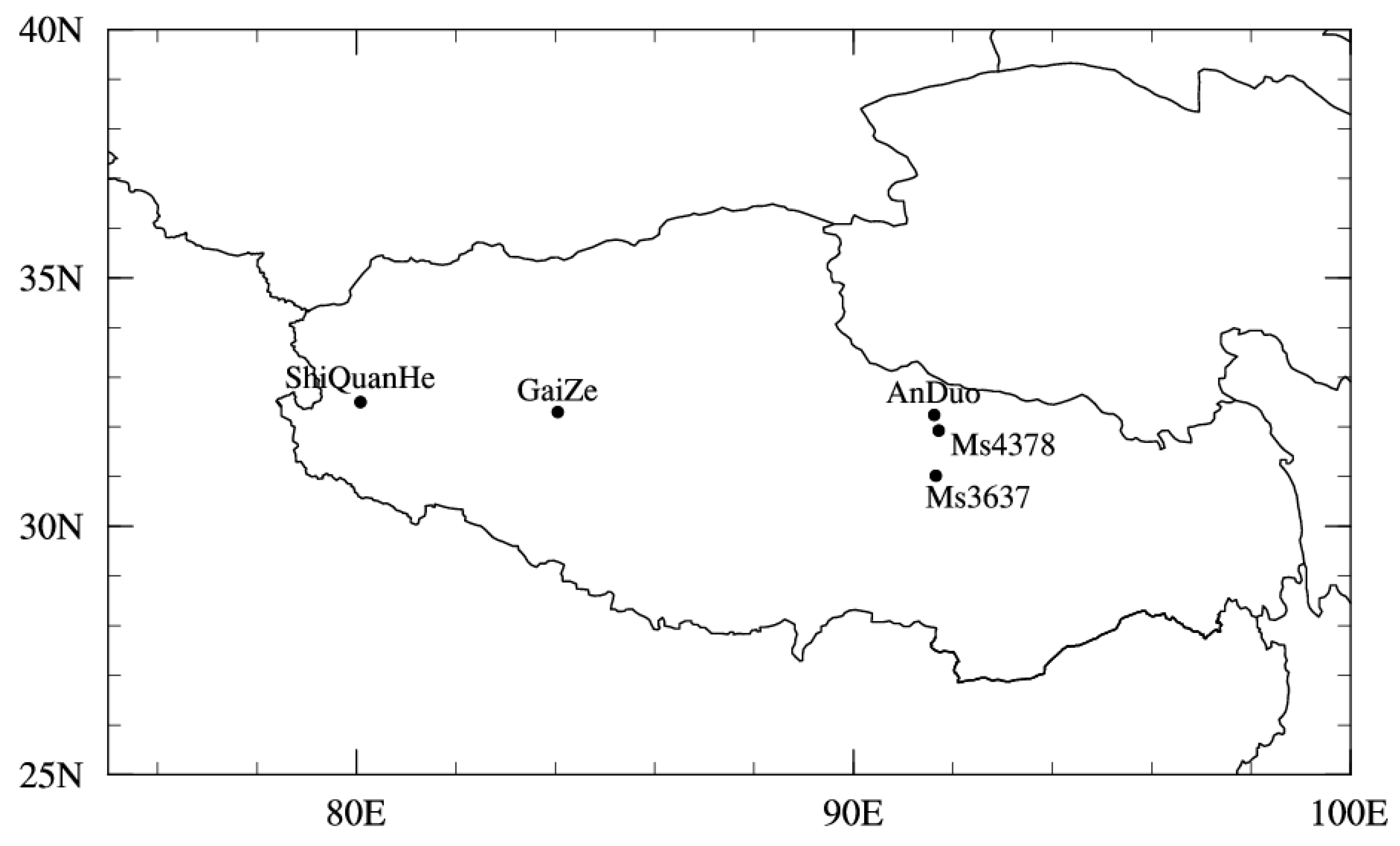
Five observational sites were chosen to characterize the land surfaces over the entire TP: AnDuo, Ms3478, Ms3637, GaiZe and ShiQuanHe (Figure 1, Table 1). Among these sites, AnDuo, Ms3478 and Ms3637 were wetter alpine meadow sites in the central and eastern TP. GaiZe and ShiQuanHe were drier alpine desert sites in the western TP.
At the five sites, in situ data collected within the intensive observation period (May–September, 1998) of the GAME-Tibet (GEWEX Asian Monsoon Experiment in the Tibetan Plateau) [42] were used as the forcing dataset to conduct land surface modeling. Limited by the incompleteness of observational data, different simulated (study) periods were chosen at different sites. The simulated (study) periods at each site are listed in Table 1. To avoid the effects of initial errors, the forcing data on the first day of the simulated period were utilized repeatedly for the model spin-up of 100 days. During the spin-up period, parameter perturbations were not superposed.
2.2. Common Land Surface Model (CoLM)
The CoLM is a sophisticated model developed by Dai et al. [37] that comprehensively describes biophysical, biochemical, ecological and hydrological processes. In addition, the energy and water transmissions among soil, vegetation, snow and atmosphere are also well considered. Several studies have confirmed that different land surface processes could be reasonably captured by CoLM [43,44,45].
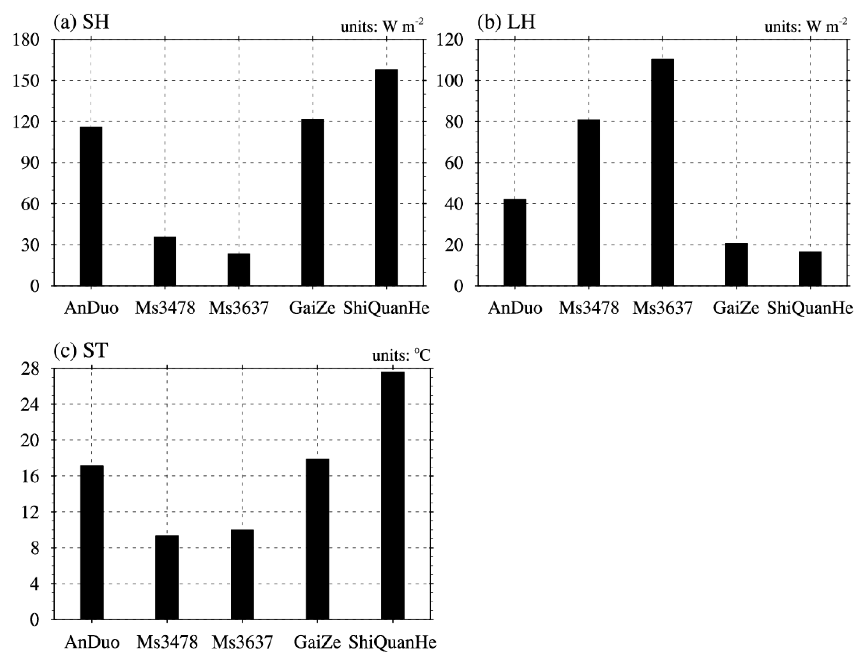
Notably, ST (i.e., soil temperature for the top 10 cm soil layer) is not a direct output of the CoLM model. As the depth of the first three soil layers in the CoLM was 9.06 cm, ST in this study was determined to be the weighted average of the soil temperature in the first three soil layers according to the soil layer thicknesses. Figure 2 shows the simulated SH, LH and ST averaged during the study periods for different TP sites. Additionally, due to the limited observations, evaluations of the CoLM model’s ability to simulate surface heat fluxes at some of the five study sites are provided in the Supplementary Material. As model parameters associated with soil and vegetation are not available from observations, simulations are conducted by running the CoLM model with the default values of these model parameters. It is well known that errors exist in the model default parameters, which are usually acquired from other variables based on theoretical or empirical considerations or prescribed by look-up tables. Therefore, errors inevitably appear in the simulated surface heat fluxes even though the model parameterizations are reasonable. By comparing observations and simulations for SH from three observational sites, Ms3637, Ms3478 and AnDuo, it can be seen that although peak values in the afternoon at the Ms3637 and Ms3478 sites are not simulated well and SH in the evening is overestimated at the AnDuo site, the diurnal cycle of SH is well captured (see Figure S1 in the Supplementary Material). For LH, similar to SH at Ms3478 and AnDuo, the diurnal cycle is well simulated (see Figure S2 in the Supplementary Material). At the AnDuo site, the peak values are not well simulated. These results at least justify that the CoLM model can capture the surface heat fluxes in terms of the diurnal cycle. Generally, the modeling errors for SH and LH can be attributed to improper model parametrizations; however, errors arising from model parameters cannot be excluded. Researches have shown that specification of the default parameters may cause significant errors in the surface energy budget [35,46,47]. Our study will focus on the simulation errors caused by model parameters. Modeling errors due to model parameterizations are not in the scope of this study.
2.3. Methods
2.3.1. The Conditional Nonlinear Optimal Perturbation Related to Parameters (CNOP-P) Approach
The CNOP-P approach is developed specifically for investigating the simulation or prediction errors due to model parameters [38]. CNOP-P is a type of parameter errors that satisfy certain constraint conditions and could lead to maximal simulation or prediction errors at a target time. To date, the CNOP-P approach has been extensively employed in studies of ENSO predictability [48], the predictability of the Kuroshio large meander [49], grassland ecosystems [50,51], terrestrial ecosystems [52,53,54,55], land surface hydrology [56,57], parameter calibrations [58,59] and parameter sensitivity analyses of numerical models [39,40,41].
Next, the CNOP-P approach is briefly introduced for readers. For more information, readers can refer to Mu et al. [38], who first proposed this approach. Assume that the state variable U satisfies the nonlinear differential equations as follows:
where U0 represents the initial value of the state variable U, P represents a parameter vector and F is a nonlinear operator. Let Mt be the propagator of the nonlinear differential equations above from the initial time 0 to t. Then, the solution at time t, U(t), satisfies U(t) = Mt (U0, P). A perturbation to the initial parameter vector P, denoted as p, is considered. Now, the solution of Equation (1) is Mt (U0, P + p) and can be characterized by U(t) + u(t), where u(t) (i.e., Mt (U0, P + p) − Mt (U0, P)) shows the change in the reference state U(t) due to p.
In terms of a target time T and norm , the perturbation is called a CNOP-P with the constraint condition if and only if the following is true:
where
P is a reference state of the parameter vector and represents the standard parameter values in the model, p is the perturbation to the reference state of the parameter vector and represents the parameter vector error and is the feasible domain of the parameter perturbation p. In addition, the cost function J depicts the variation magnitude of the reference state U due to the parameter errors p. As a result, the CNOP-P is a type of parameter perturbation, the nonlinear evolution of which attains the maximum of the cost function J at time T. The cost function value with the CNOP-P represents the maximal variation magnitude of the reference state due to parameter perturbations. In this study, this type of cost function value is the maximal uncertainty extent (i.e., simulation or prediction errors) in numerical simulations due to parameter errors.
In our study, the differential evolution (DE) [60] algorithm, an efficient and derivative-free method, was applied to compute the CNOP-Ps as well as the corresponding cost function values (i.e., the maxima of the cost function).
2.3.2. The Sensitivity Analysis Framework for the Model Parameter Combination Based on the CNOP-P
To determine the most sensitive parameter combination in the numerical models, Sun and Mu [39] proposed a novel and flexible sensitivity analysis framework based on the CNOP-P. This sensitivity analysis framework inherits a merit from the CNOP-P approach, which is that nonlinear interactions among parameters are considered. In general, this framework contains three steps. The first step is to choose parameters that can be acquired via direct or indirect observations. The second step is to implement the sensitivity analysis for a single parameter based on the CNOP-P and then remove several insensitive parameters. The sensitivity for each parameter is measured by the maximal uncertainty extent in the numerical simulations due to a single parameter error, which can be obtained using the CNOP-P approach. The greater the maximal uncertainty extent is (i.e., value of the cost function under the CNOP-P), the more sensitive the corresponding parameter will be. In this step, only one parameter is perturbed, and interactions among parameters are not considered. In the third step, a sensitivity analysis for multiple parameters based on the CNOP-P is conducted to determine the sensitivities of parameter combinations with a specified parameter size. Similar to the second step, for each parameter combination, the sensitivity depends on the maximal uncertainty extent in the numerical simulations due to errors of parameters from the parameter combination, which can also be obtained using the CNOP-P approach. The greater the maximal uncertainty extent is (i.e., the cost function value under the CNOP-P), the more sensitive the corresponding parameter combination will be. As multiple parameters are perturbed simultaneously, interactions among parameters are considered in identifying the sensitivities of parameter combinations. Finally, the most sensitive parameter combination is determined from the relatively sensitive parameters that are identified in the second step.
Additionally, both the number of relatively sensitive parameters identified in the second step and the parameter size of the most sensitive parameter combination in the third step could be arbitrarily specified according to the users’ requirements. This reflects the flexibility of the three-step sensitivity analysis framework in detecting the most sensitive parameter combinations.
2.3.3. The OAT (One-at-a-Time) Approach
For comparison with the sensitivity analysis results for a single parameter using the CNOP-P approach, the one-at-a-time approach (OAT) [61] is also employed to determine the sensitivity of a single parameter. In this method, when a parameter is perturbed, the other parameters remain unchanged. Thus, the OAT method ignores the interactions among parameters. Then, the percentage variation (Pervar) in a model prognostic variable owing to the perturbation in one parameter could be computed as follows:
where CON is the control value of a model variable simulated without parameter perturbations, and PERT is the value simulated with a 10%, 20% or 30% change in only one parameter. Obviously, for the target model prognostic variable, the greater the Pervar is, the more sensitive one parameter will be.
At a specified observational site in our research, the value of CON is fixed. Therefore, the absolute error of a model prognostic variable caused by the perturbed parameter (i.e., abs(PERB−CON)) is applied to directly measure the sensitivity of a parameter. The greater the absolute error is, the more sensitive one parameter will be.
2.4. Experimental Design
In this research, 28 parameters associated with soil, vegetation and snow were selected from the CoLM model and described in Table 2. The parameters along with their feasible ranges were ascertained according to the studies by Dai et al. [37], Li et al. [62] and Sun et al. [41]. The CoLM model has 10 soil layers, and thus, soil-related parameters should change with the soil layers. Consequently, to represent the vertical soil heterogeneity, soil-related parameters were divided into parameters associated with topsoil and subsoil. Furthermore, the soil for the first five soil layers was classified as topsoil (with depths shallower than 29 cm), while the soil for the lower five soil layers was classified as subsoil (with depths deeper than 29 cm). For example, P01 represented the porosity of the upper five soil layers, and P02 represented the porosity of the lower five soil layers.
When the CNOP-P approach was applied, the study period was chosen as the simulated period, as listed in Table 1. Here, the target time T indicates a period, i.e., the entire study period. In this case, the propagator at target time T (i.e., MT) represented the state variables (SH, LH or ST) averaged over the entire study period. The cost function was chosen as the magnitude of the simulation error caused by parameter errors. During calculations of the CNOP-Ps, parameter errors existed and remained unchanged during the entire simulated period. The obtained CNOP-Ps represented the type of parameter errors that led to the maximal extent of uncertainty in the simulated state variables (SH, LH or ST) averaged over the entire study period. The physical comprehension of the cost function value under the CNOP-P was the maximal uncertainty extent in the simulations, which was also used to measure the importance and sensitivity of a single parameter or parameter combination.
To facilitate the application of the CNOP-P approach, all parameters were normalized to the range of [−1, 1] based on the following criteria:
In this rule, x and y are pre-normalization and post-normalization parameters, respectively. Defvalue, Maxvalue and Minvalue represent the standard, maximum and minimum values, respectively. When x = Minvalue, y = −1 and when x = Maxvalue, y = 1. When x = Defvalue, y = 0. In that way, the constraint condition in Equation (2),, changed to . This transformed constraint condition was a box constraint and conductive to the CNOP-P calculations.
During the process of screening the sensitive parameter or parameter combination using the three-step sensitivity analysis framework based on the CNOP-P, three variables, namely, SH, LH and ST, were successively chosen as the state variable of the cost function in the CNOP-P approach. Limited by computational resources, the number of relatively sensitive parameters in the second step and the parameter size of the most sensitive parameter combination in the third step were set to 8 and 4, respectively. That is, via the sensitivity analysis for a single parameter in the second step, all 28 parameters were ranked, and eight relatively sensitive parameters were selected. Instantly, (i.e., 70) groups of parameter combinations with four parameter members could be derived from the abovementioned eight relatively sensitive parameters. Then, through the sensitivity analysis for multiple parameters in the third step, all (i.e., 70) groups of parameter combinations were ranked, and the most sensitive four-parameter combination could be identified.
Moreover, we also used the OAT approach [61] to investigate the sensitivity of a single parameter. In the optimization process of the CNOP-P approach, the maximal or minimal value of a parameter may be sampled; for fairness, the maximal and minimal values of one parameter are both applied as the perturbed parameter values in the OAT approach. In addition, between the absolute errors due to the two perturbed parameter values, the greater one is used to measure the sensitivity of each parameter.
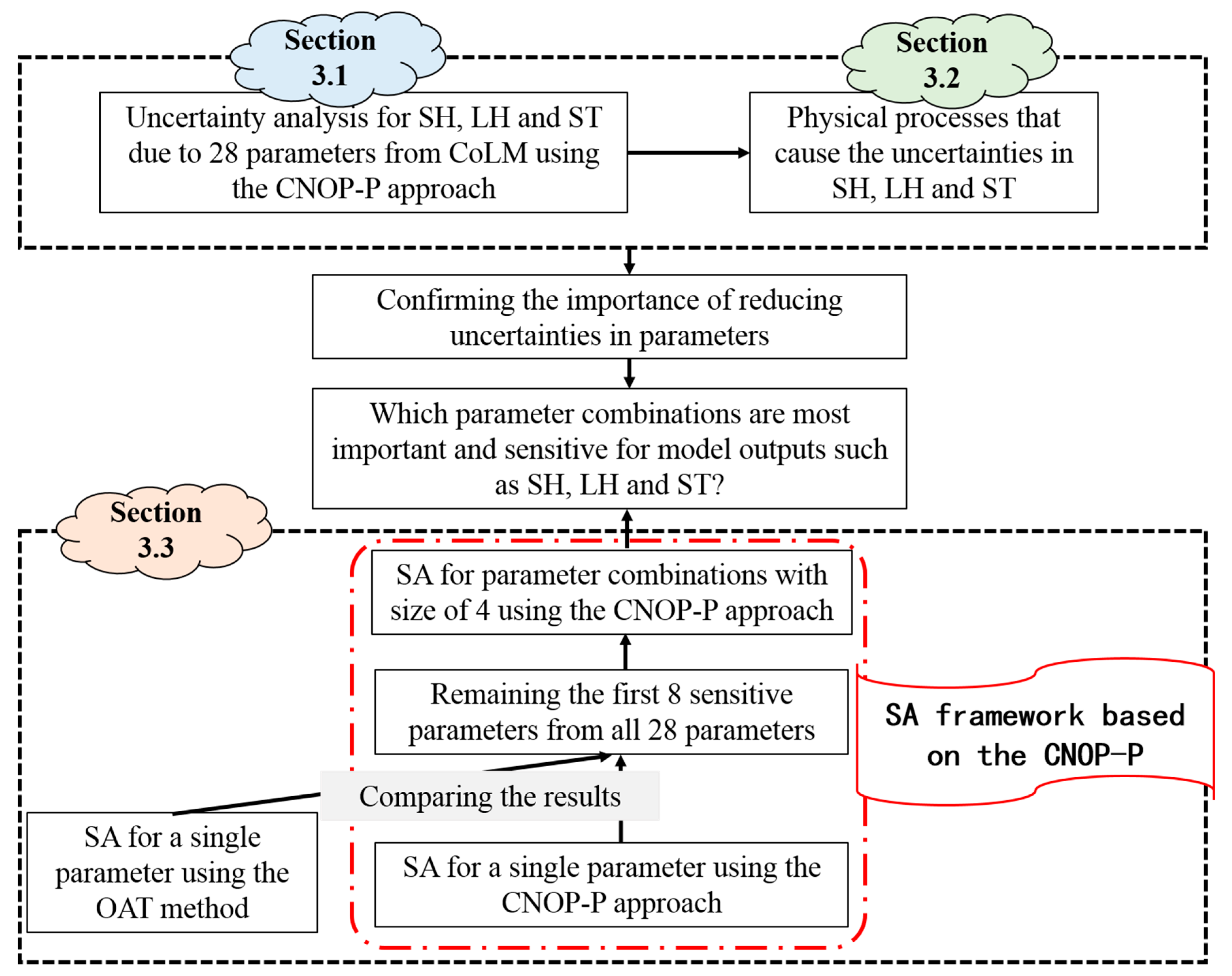
In summary, to achieve the two objectives proposed in the introduction section, the flow chart of this study is described in Figure 3. First, the influences of uncertainties from the 28 parameters of CoLM on the simulated SH, LH and ST were quantified using the CNOP-P approach, which would be shown in Section 3.1. Then, the physical processes that cause the uncertainties in SH, LH and ST would be analyzed (Section 3.2). The results from the above two sections can provide evidence for the necessity and importance of reducing uncertainties in the model parameters by means of data assimilation or calibration methods. Finally, to identify parameters that are crucial for model performance, the sensitivity analysis is conducted step by step using the CNOP-P approach, and the most important and sensitive parameter combinations will be identified (Section 3.3). Additionally, it should be noted that the OAT method is only applied to conduct a single parameter sensitivity analysis for ranking the sensitivities of parameters, which would serve as a comparison and further confirm the results from the sensitivity analysis for a single parameter using the CNOP-P approach. When the sensitivities of parameter combinations are identified, only the CNOP-P approach is employed.
3. Results and Analyses
3.1. Uncertainties in SH, LH and ST due to Parameter Uncertainties
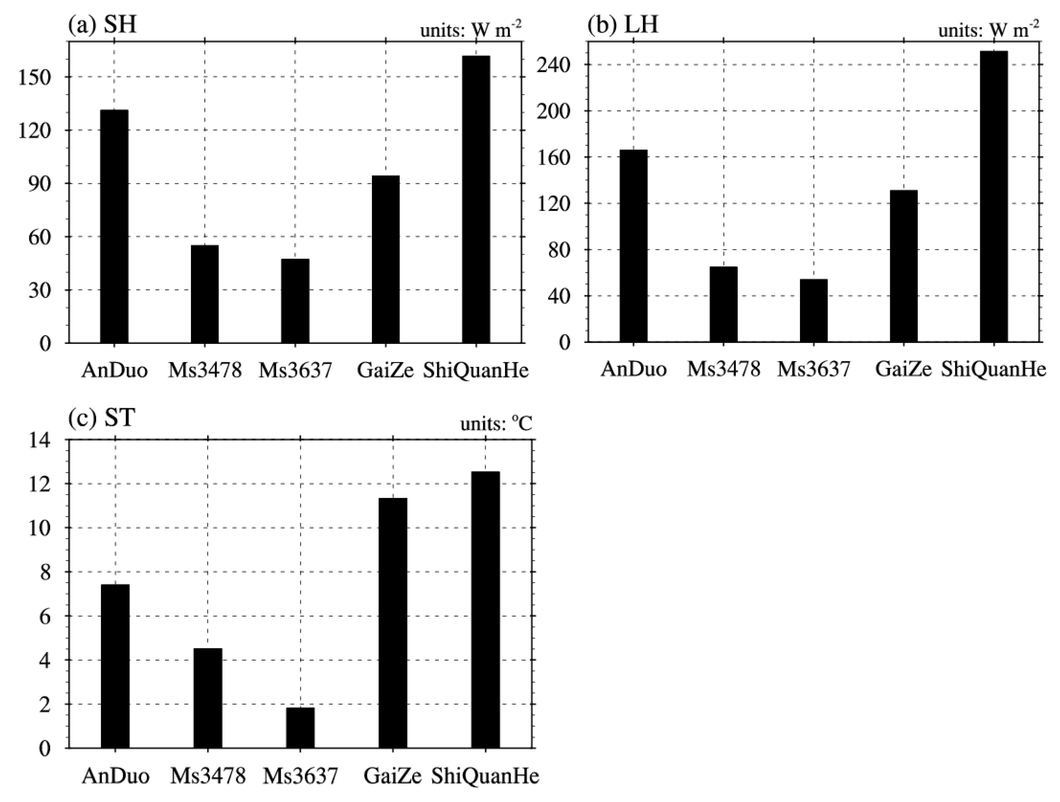
From Section 2, we know that uncertainties in numerical simulations caused by parameter errors alone could be bounded by the cost function values under the CNOP-Ps, which were obtained through the optimization procedure of the CNOP-P approach. Figure 4a shows the maximal uncertainties in the simulated SH at five Tibetan sites due to errors in the 28 selected model parameters. At the AnDuo and ShiQuanHe sites, the uncertainties (more than 130 W m−2) were greater than those at the other Tibetan sites. At the Ms3478 and Ms3637 sites, uncertainties were smaller (less than 60 W m−2). For uncertainties in the simulated LH, similar results were determined (Figure 4b). At the AnDuo and ShiQuanHe sites, the uncertainties were larger than those at the other Tibetan sites, exceeding 160 W m−2. In addition, at the Ms3478 and Ms3637 sites, the uncertainties were smaller, less than 65 W m−2. Furthermore, the maximal uncertainties associated with ST are shown in Figure 4c. At the GaiZe and ShiQuanHe sites, the uncertainties exceeded 10 °C. However, at the Ms3637 site, this kind of uncertainty decreased to approximately 2 °C.
The above results revealed that parameter errors could cause non-negligible uncertainties in surface heat fluxes (i.e., SH and LH) as well as soil temperature (i.e., ST). In addition, at any of the five Tibetan sites, if parameter errors could cause greater (smaller) uncertainties in any one of the three state variables (SH, LH and ST), then they could lead to greater (smaller) uncertainties in the remaining two state variables. This can be explained by the close correlations among SH, LH and ST constrained by the surface heat balance. Moreover, no matter which state variable was considered in the CNOP-P approach, uncertainties at the AnDuo, GaiZe and ShiQuanHe sites were greater and smaller at the remaining two sites (i.e., Ms3478 and Ms3637).
3.2. Physical Processes Contributing to the Uncertainties in SH, LH and ST
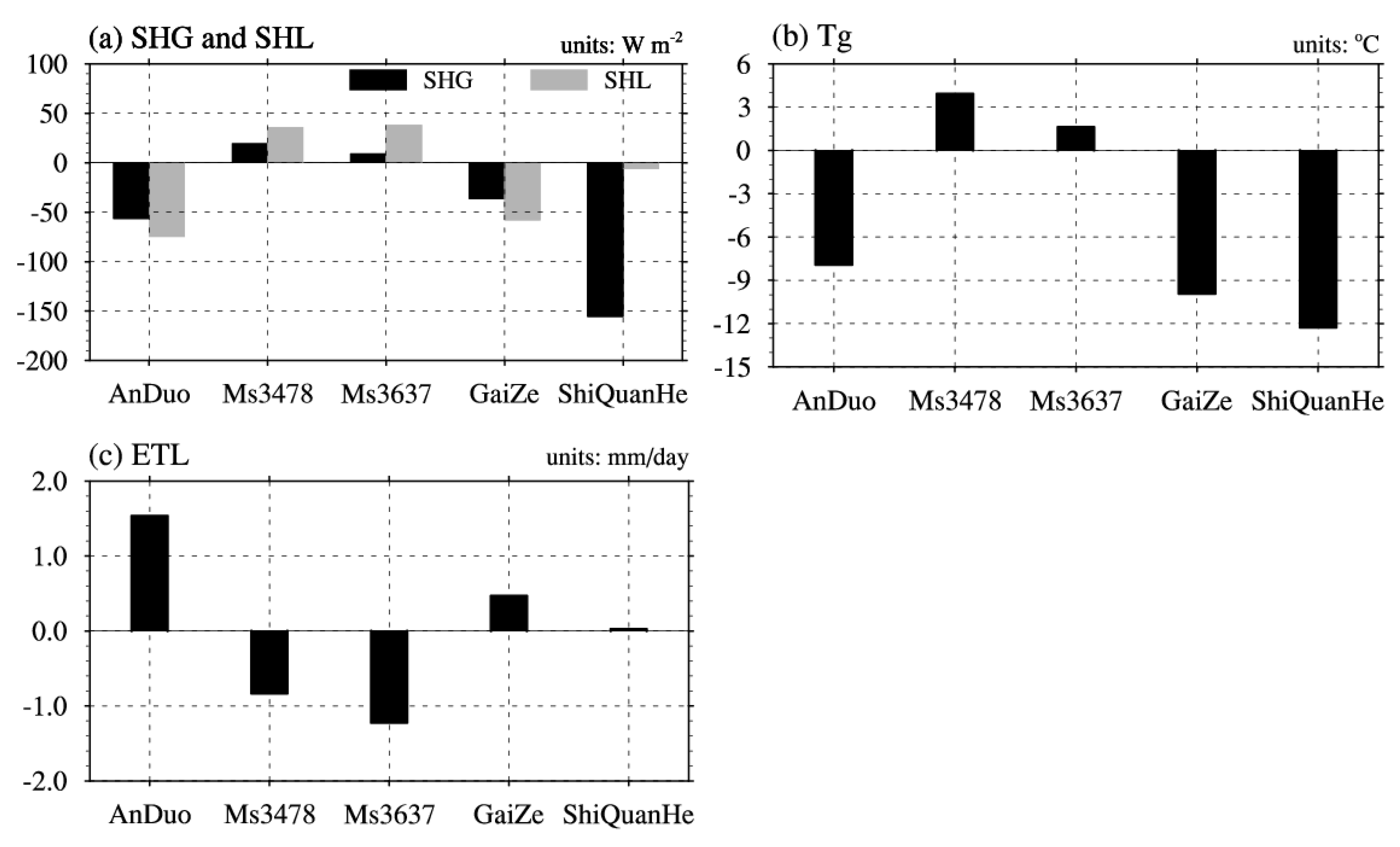
Next, physical processes that contributed to the maximal uncertainties in SH, LH and ST caused by parameter errors will be discussed. In the CoLM model, SH is calculated as the sum of the sensible heat flux from both ground (SHG) and leaves (SHL; i.e., SH = SHG + SHL). SHG depends on the temperature gradients between the ground surface and canopy, while SHL is determined by the temperature gradients between the leaves and canopy. Changes in evapotranspiration from leaves (ETL) could be used as an indicator of variations in leaf temperature. An increase (decrease) in ETL signifies a decrease (increase) in leaf temperature. Thus, changes in the ground surface temperature (Tg) and ETL under CNOP-Ps will be explored to qualitatively account for the uncertainties in SH due to parameter errors. For LH, it depends on evapotranspiration from the canopy to atmosphere (ET), which consists of evaporation from ground (Eg) and evapotranspiration from leaves (ETL; i.e., ET = Eg + ETL). Therefore, variations in ET, Eg and ETL under CNOP-Ps will be analyzed to demonstrate the uncertainties in LH. As changes in ST are controlled by the ground heat flux (GHF), variations in GHF under CNOP-Ps will be investigated to illustrate the uncertainties in ST.
Figure 5 shows the changes in SHG, SHL, Tg and ETL under CNOP-Ps relative to their respective reference states when SH was chosen as the objective state variable in the CNOP-P approach. At the AnDuo and GaiZe sites, changes in SHG and SHL jointly resulted in variations in SH (Figure 5a). For the two sites, Tg was greatly reduced (Figure 5b), contributing to the reduction in temperature gradients between the ground surface and canopy and then the decrease in SHG. Similarly, the augmentation of ETL indicated a decrease in leaf temperature (Figure 5c), which was conducive to the reduction in temperature gradients between the leaves and canopy and then a decrease in SHL. In general, at the AnDuo and GaiZe sites, the uncertainties in SH due to CNOP-Ps were attributed to the dramatic reduction in the ground surface temperature and decrease in the leaf temperature related to the enhanced evapotranspiration from leaves. At the Ms3478 and Ms3637 sites, changes in SH largely originated from variations in SHL (Figure 5a), which were mainly caused by the increased temperature gradients between leaves and canopy associated with the reduced ETL (Figure 5c). For the ShiQuanHe site, changes in SH were dominated by the changes in SHG, which were caused by the reduced temperature gradients between the ground surface and canopy due to the strongly decreased Tg (Figure 5b).
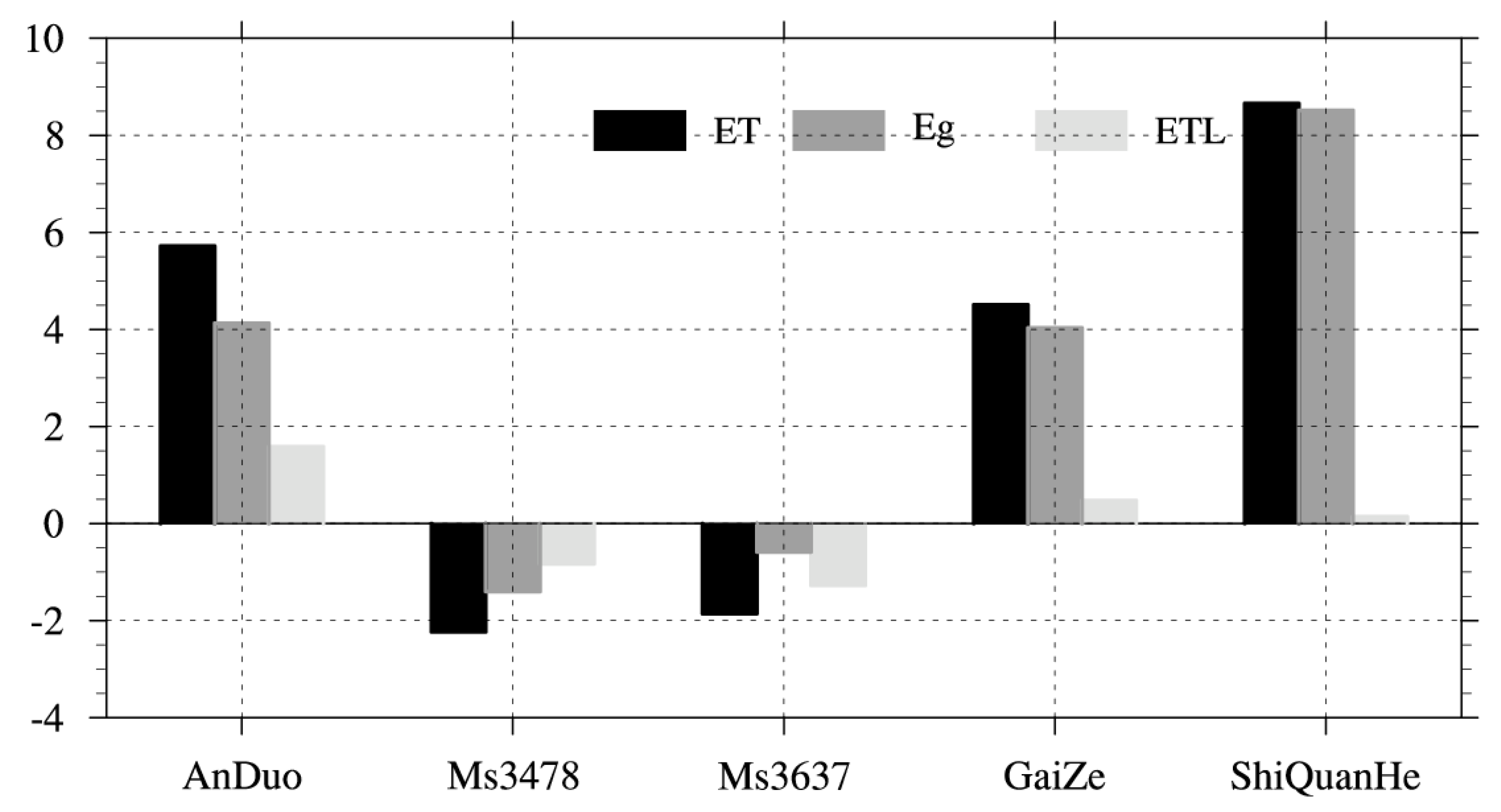
When physical processes accounting for the uncertainties in LH under CNOP-Ps were explored, ET, Eg and ETL were analyzed. The changes in the above three variables due to CNOP-Ps are shown in Figure 6. At different sites, the change signs of LH were the same as those for ET. At the AnDuo, Ms3478, GaiZe and ShiQuanHe sites, changes in ET largely resulted from variations in Eg. Furthermore, at the AnDuo, GaiZe and ShiQuanHe sites, the enhanced Eg primarily contributed to the uncertainties in LH, while at the Ms3478 site, the restrained Eg mainly led to the changes in LH. However, at the Ms3637 site, the inhibited ETL mainly contributed to the variations in LH.
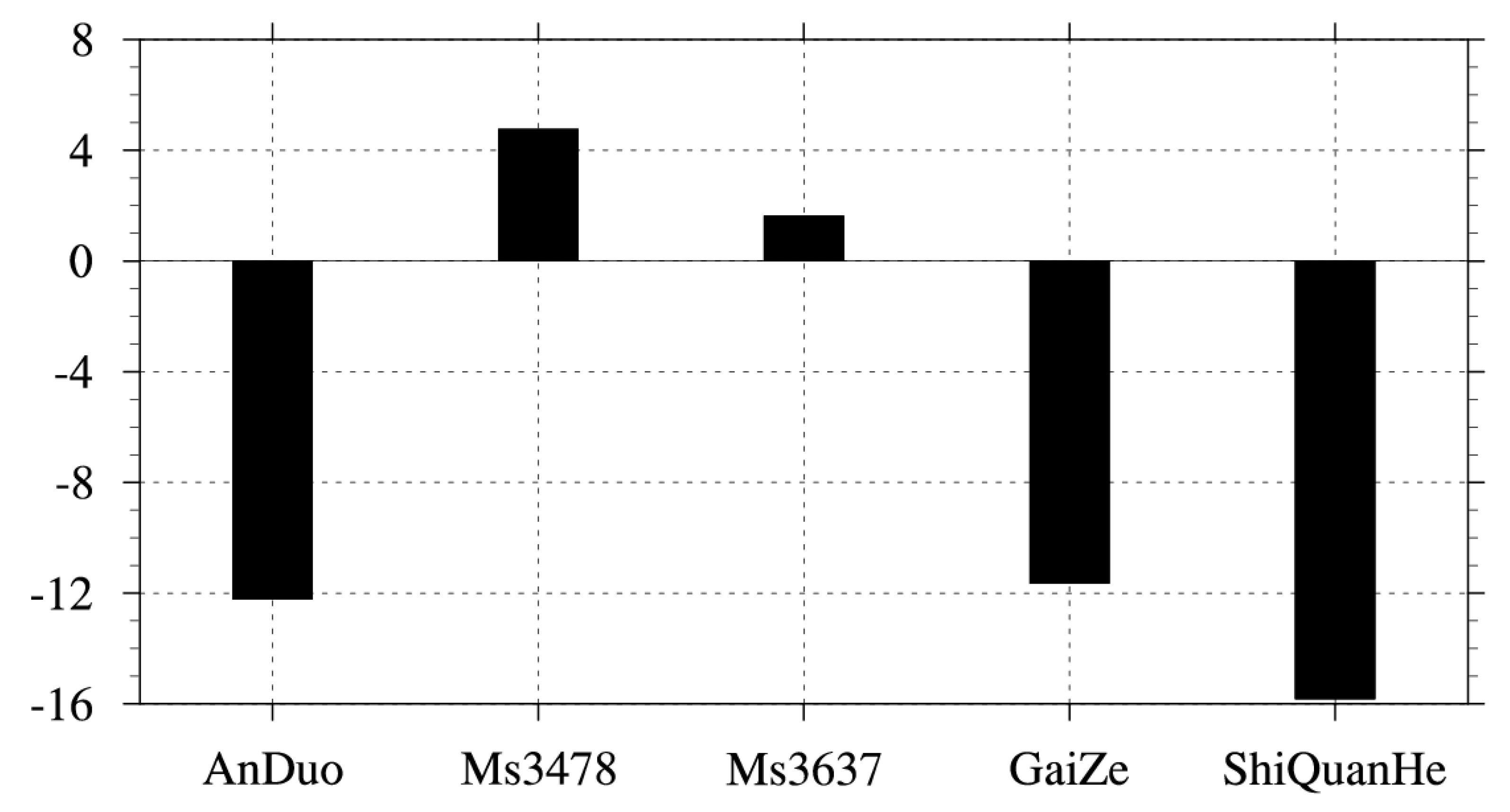
As the changes in ST were determined by GHF, CNOP-Ps altered the ST mainly by influencing GHF. In Figure 7, changes in GHF under CNOP-Ps were exhibited. The change signs of ST under CNOP-Ps were the same as those for GHF. At the AnDuo, GaiZe and ShiQuanHe sites, the reductions in GHF indicated that less heat could be absorbed by the surface soil, thus decreasing ST. Furthermore, at the Ms3478 and Ms3637 sites, the increased GHF provided more heat flux for warming the surface soil, which is conductive to the increase in ST.
From Section 3.1 and Section 3.2, large errors might appear in simulations due to inappropriate parameters. At some sites, the errors were very large, which seems unrealistic. For example, at the ShiQuanHe site, the error in ET (i.e., variation in ET) reached approximately 8.5 mm/day due to the parameter errors characterized by the CNOP-P when LH was chosen as the objective state variable in the CNOP-P approach (Figure 6). However, at this site, the large error in ET explained the large error in LH (Figure 4). Considering the large error in LH, the error in ET is reasonable and should be large. It is important to note that the large error in ET or LH or other model variables here was a kind of simulation error that could appear only when CNOP-Ps were specified as parameter errors in the CoLM model. CNOP-Ps are acquired to make the cost function (i.e., the simulated error of the target model output) attain its maximum through an optimization procedure, and fluctuate in the feasible range of parameter errors. As the realistic parameter errors are unknown, we are unsure whether parameter errors characterized by CNOP-Ps can appear in reality. Furthermore, we were also unsure whether the errors in simulations due to parameter errors characterized by CNOP-Ps were realistic. However, we were sure that when CNOP-Ps are deemed as parameter errors, these large errors would occur in the simulations.
3.3. Identification of the Most Sensitive and Important Parameter Combination
The previous section showed the maximal uncertainties in the simulated SH, LH and ST owing to parameter errors and addressed the significant influence of parameter uncertainties on surface heat fluxes and soil temperature modeling. Due to the large number of parameters in complex land surface models as well as the limited human and computational resources, it is impractical to reduce uncertainties in all parameters. Sensitivity analyses should be conducted to first determine the relatively sensitive parameters. In the following section, different approaches, i.e., the three-step sensitivity analysis framework based on the CNOP-P method and the traditional OAT method will be applied to identify the sensitivity and importance of parameters. Furthermore, both the OAT method and the CNOP-P approach were employed to determine the sensitivity of a single parameter. Then, according to the results from a single parameter sensitivity analysis, several insensitive parameters could be removed from all 28 parameters. Due to the limited computational resources, only the first eight sensitive parameters were kept for use in the last step of the sensitivity analysis framework built on the CNOP-P method. Finally, from the remaining eight relatively sensitive parameters, the most sensitive parameter combination with the parameter size of four would be identified. When the sensitivity of a parameter combination was measured, only the CNOP-P approach was employed, and the interactions among parameters were considered.
3.3.1. SH
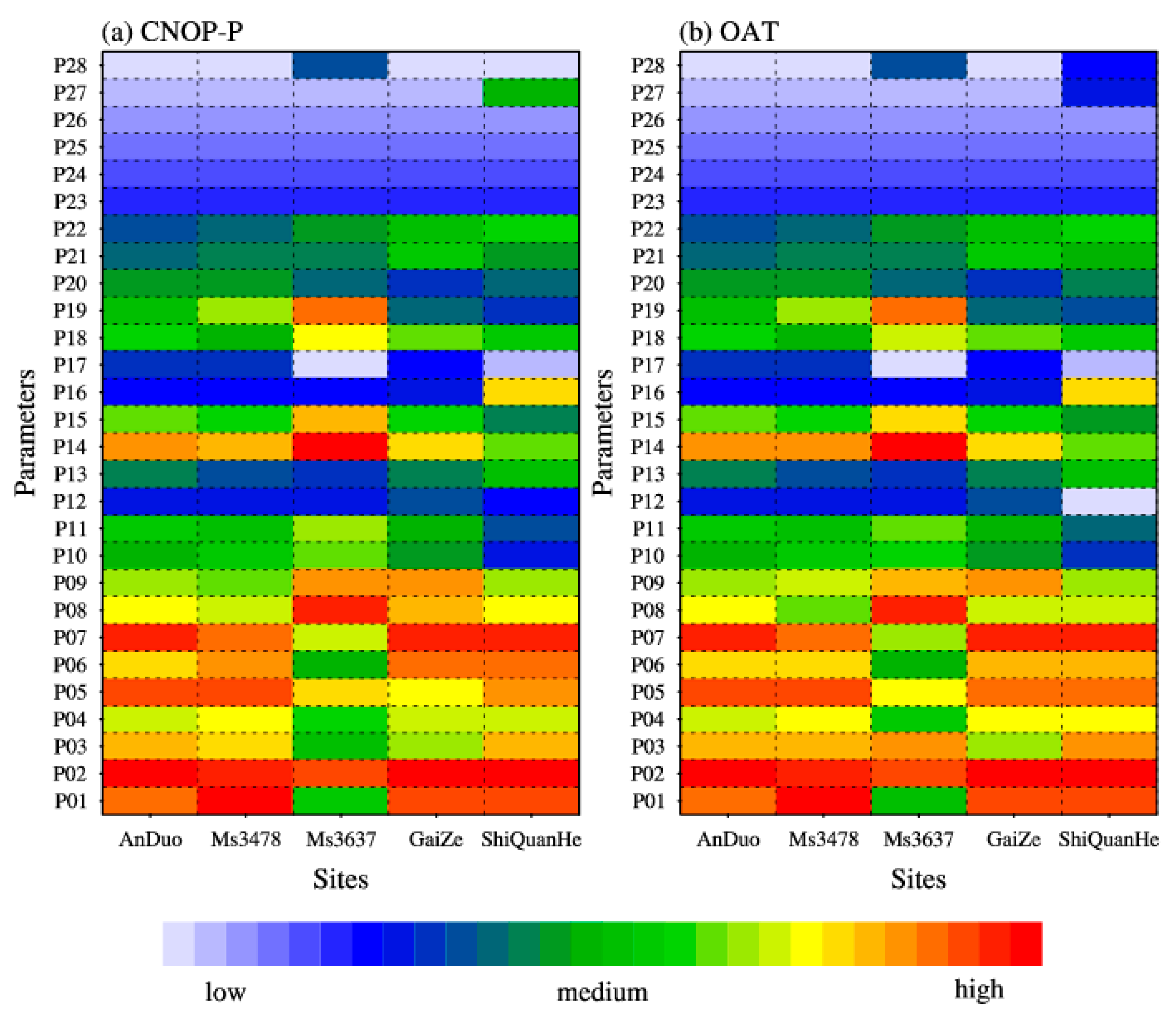
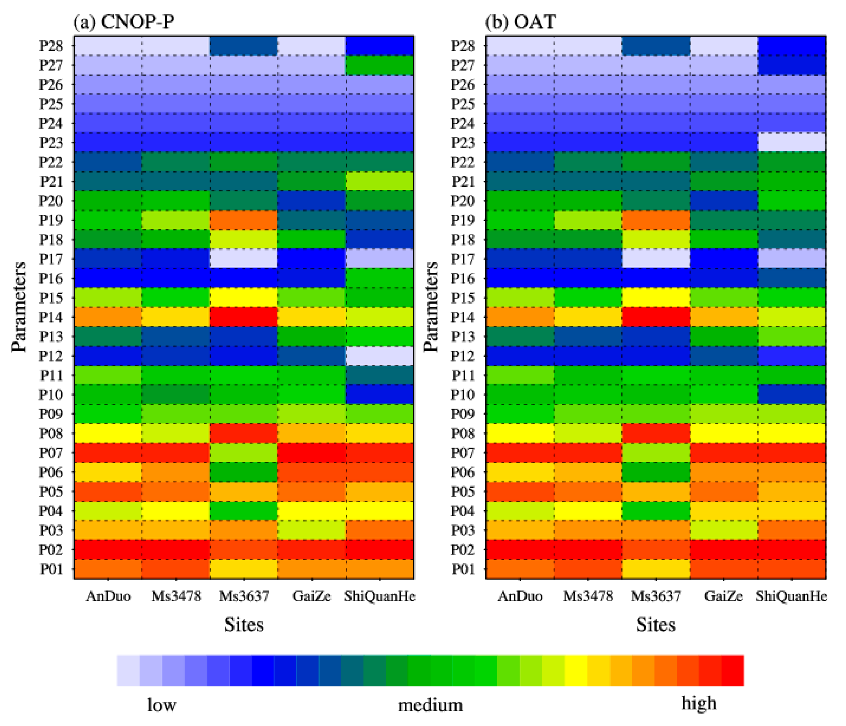
In the sensitivity analysis framework based on the CNOP-P method, after determining the information about the selected parameters, the subsequent step was to conduct a sensitivity analysis for a single parameter. Figure 8a shows the results of a single parameter sensitivity analysis for SH using the CNOP-P approach. At all sites, except the Ms3637 site, sensitivities of P01 (i.e., the porosity of the upper soil layer), P02 (i.e., the porosity of the lower soil layer) and P07 (i.e., the saturated hydraulic conductivity of the upper soil layer) always ranked as the top five. The OAT method was also used to conduct a single parameter sensitivity analysis for SH, and the results also revealed the similar importance and sensitivity of P01, P02 and P07 (Figure 8b). In the Clapp and Hornberger empirical formulas [63] applied by the CoLM model, P01 and P02 were used to obtain the soil hydraulic conductivity and matric potential, both of which are key factors influencing the simulation of soil moisture. In addition, the formula of hydraulic conductivity also depends on the saturated hydraulic conductivity. As the simulation of SH is closely related to the modeled soil moisture [65], the three parameters P01, P02 and P07 could alter the soil moisture through soil hydraulic conductivity and matric potential, and thus had a significant influence on SH. This is consistent with the findings of our previous research [66], which revealed that porosity and saturated hydraulic conductivity were important and sensitive parameters for surface soil moisture modeling on the Tibetan Plateau.
Through the single parameter analysis based on the CNOP-P approach, the first eight sensitive parameters can be acquired. Then, by the multiple parameter analysis built on the CNOP-P method, the most sensitive and important parameter combinations with four member parameters for SH were identified from the eight obtained relatively sensitive parameters. Table 3 lists the most sensitive parameter combinations at different Tibetan sites and the maximal uncertainties these parameter combinations could induce. The most sensitive parameter combinations varied among sites. At nearly all of the sites, three or four soil texture-related parameters were contained in these identified combinations. Only at the wetter sites, such as AnDuo and Ms3637, were parameters related to vegetation contained in the most sensitive parameter combinations. Furthermore, even if the combinations had only four parameters, the potential uncertainties due to these four-parameter combinations accounted for a large proportion of the uncertainties that the 28 parameters could cause.
3.3.2. LH
For LH, the results of a single parameter sensitivity analysis for LH using the CNOP-P approach also addressed the important and sensitive roles of P01, P02 and P07 (ranking as the top five) at all sites except the Ms3637 site, similar to the results for SH (Figure 9a). In addition, the OAT method for LH confirmed this point (Figure 9b). Considering that both soil moisture and SH are strongly linked to LH [65], it is physically reasonable that perturbations to P01, P02 and P07 could greatly affect LH.
Using the results of the single parameter sensitivity analysis, through the last step of the sensitivity analysis framework based on the CNOP-P method, the most sensitive and important parameter combinations with four member parameters were screened out for LH from the remaining eight relatively sensitive parameters, which are displayed in Table 4. Similar to the results for SH, the most sensitive parameter combinations varied among sites. At nearly all of the sites, in these identified combinations, three or four parameters were soil texture related. Only at the wetter sites, such as AnDuo and Ms3637, were parameters related to vegetation contained in the most sensitive parameter combinations, similar to the SH results. In addition, the uncertainties due to the parameter combination with four parameters were comparable to those caused by 28 parameters.
3.3.3. ST
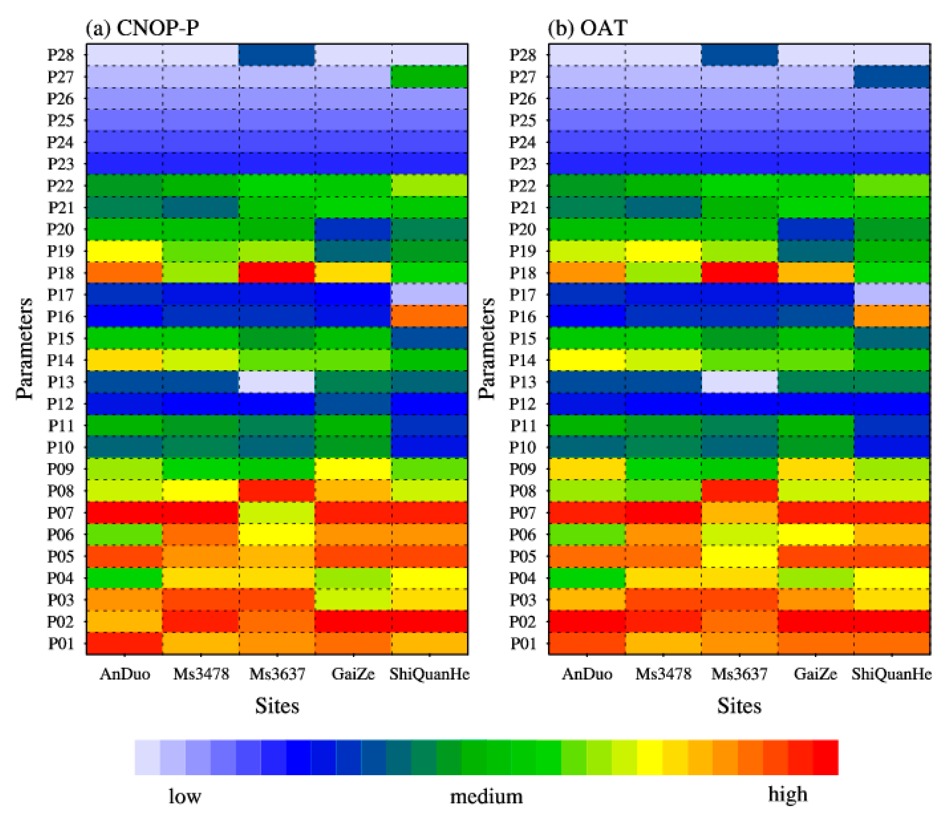
The results of the single parameter sensitivity analysis for ST using the CNOP-P approach are shown in Figure 10a. At most sites, the first five sensitive parameters always included P02 and P07. The OAT method was used to determine the sensitivity of a single parameter, also indicating the sensitivity and importance of P02 and P07 (Figure 10b). As discussed above, P02 and P07 could exert important influences on soil moisture by affecting soil hydraulic conductivity and matric potential and thus have considerable impacts on ST.
Using the multiple parameter analysis based on the CNOP-P method, the most sensitive parameter combinations with four parameters for ST were identified from the eight relatively sensitive parameters obtained from the results of a single parameter sensitivity analysis. Table 5 shows the most sensitive parameter combinations at different Tibetan sites and the maximal uncertainties these parameter combinations could induce. The most sensitive parameter combinations varied among sites. At nearly all of the sites, three or four soil texture-related parameters were contained in these identified combinations. Similar to SH and LH, only at the wetter sites, such as AnDuo and Ms3637, were parameters related to vegetation contained in the most sensitive parameter combinations. In addition, even if the combinations only had four parameters, the potential uncertainties accounted for a large proportion of the uncertainties that the 28 parameters could cause.
4. Summary and Future Work
To provide guidelines for the accurate representation of land surface processes over the TP in LSMs by removing the uncertainties in a smaller set of model parameters, comprehensive uncertainty and sensitivity analyses were conducted in this study for surface heat fluxes (including SH and LH) as well as soil temperature (i.e., ST) simulated by the CoLM model. First, the CNOP-P approach was used to explore the impacts of 28 uncertain model parameters on SH, LH and ST modeling. This approach is a nonlinear optimization method and could be used to evaluate the maximal uncertainties of simulations or predictions in the reasonable range of parameter errors by considering the nonlinear interactions among multiple parameters. Then, the sensitivity analysis framework based on the CNOP-P proposed by Sun and Mu [39] was used to evaluate the sensitivities of a single parameter or parameter combination. This sensitivity analysis framework inherited the merit of the CNOP-P approach where the nonlinear interactions among parameters were considered, and could be used to identify the sensitivities of parameter combinations. For comparison, the OAT method, in which interactions among parameters were ignored, was also used to investigate the sensitivities of parameters. Five observational sites, namely, AnDuo, Ms3478, Ms3637, GaiZe and ShiQuanHe, were selected to represent the land surfaces over the TP. The first three sites were typical alpine meadows situated in the central and eastern TP, and the last two were typical alpine deserts located in the western TP.
Within the TP, the simulation uncertainties of LSMs caused by the model structure were addressed in a number of studies, while those associated with model parameters received little attention. Our study focused on the simulation uncertainties due to only model parameters. Numerical results based on the CNOP-Ps showed that parameter errors owned the ability to result in considerable simulation uncertainties in surface heat fluxes (i.e., SH and LH) as well as soil temperature (i.e., ST). For example, at the AnDuo site, the uncertainties in SH, LH and ST were 131.23 W m−2, 166.08 W m−2 and 7.41 °C, respectively. Due to the close relationships among SH, LH and ST constrained by the surface heat balance at each of the five Tibetan sites, greater (smaller) uncertainties in any one of the three state variables (SH, LH and ST) meant greater (smaller) uncertainties in the remaining two state variables. Generally, uncertainties at the AnDuo, GaiZe and ShiQuanHe sites were greater, and smaller at the remaining two sites (i.e., Ms3478 and Ms3637). The physical processes that primarily contributed to the simulation uncertainties were also analyzed and shown to vary among sites.
The simulation uncertainties due to model parameters were confirmed to be non-neglectable. To improve the model performance from the view of model parameters, the most sensitive parameter combinations were identified using the three-step sensitivity analysis framework based on the CNOP-P, and the parameter size of parameter combinations was set to 4. The results showed that although the most sensitive parameter combinations only had four parameters, the potential simulation uncertainties due to these four-parameter combinations accounted for a large proportion of the uncertainties that the 28 parameters could cause. In addition, the most sensitive parameter combinations identified varied with the target state variables and sites. However, they also bore some similarities. For any of the three state variables, at nearly all of the sites, three or four members from the most sensitive combinations were soil texture related. Consistent with the study by Li et al. [67], their sensitivity analysis results showed that soil parameters were generally more sensitive than vegetation parameters over the central TP for the Noah with Multiple Parameterizations (Noah-MP) LSM, and the dominant role of soil parameters was determined in the simulated land surface energy fluxes and soil temperature. This indicated that if the soil texture-related parameters were properly assigned, SH and LH together with ST could be better captured by LSMs, at least by the CoLM model. Furthermore, only at the wetter sites, such as AnDuo and Ms3637, were parameters related to vegetation contained in the most sensitive parameter combinations for SH, LH and ST.
In future work, based on the most sensitive parameter combinations identified for SH, LH and ST, studies on parameter estimations through multiobjective or single-objective optimization will be conducted to improve the performance of the CoLM model over the TP and to further verify the important role of the most sensitive parameter combinations. In addition, the parameter size of the most sensitive parameter combinations could be amplified, and then, more important parameters would be identified.
Supplementary Materials
The following are available online at https://www.mdpi.com/2073-4441/11/8/1724/s1. Figure S1: Comparisons of half-hourly SH (W m−2) between observations and simulations from the CoLM model at the Ms3637 site in the study period of 1998.08.01–08.31, at the Ms3478 site in the study period of 1998.09.01–09.16, and at the AnDuo site in the study period of 1998.06.16–06.22. Figure S2: Comparisons of half-hourly LH (W m−2) between observations and simulations from the CoLM model at the Ms3478 site in the study period of 1998.09.01–09.16, and at the AnDuo site in the study period of 1998.06.16–06.22. Table S1: Observations and simulations for SH at Ms3637, Ms3478, and AnDuo sites averaged in respective study periods. Table S2: Observations and simulations for LH at Ms3478 and AnDuo sites averaged in respective study periods.
Author Contributions
Conceptualization, F.P. and G.S.; Methodology, F.P. and G.S.; Software, F.P. and G.S.; Validation, F.P. and G.S.; Formal analysis, F.P. and G.S.; Investigation, F.P. and G.S.; Writing—original draft preparation, F.P. and G.S.; Writing—review and editing, F.P. and G.S.; Visualization, F.P.; Supervision, G.S.
Funding
Grants from the National Key Research and Development Program of China (Nos. 2017YFA0604804), grants from the National Natural Science Foundation of China (Nos. 41675104), and Youth Innovation Promotion Association, Chinese Academy of Sciences (No. 2015060) provided the funding for this research.
Conflicts of Interest
The authors declare no conflict of interest.
References
- Duan, A.M.; Wu, G.X. Role of the Tibetan Plateau thermal forcing in the summer climate patterns over subtropical Asia. Clim. Dyn. 2005, 24, 793–807. [Google Scholar] [CrossRef]
- Ueda, H.; Kamahori, H.; Yamazaki, N. Seasonal Contrasting Features of Heat and Moisture Budgets between the Eastern and Western Tibetan Plateau during the GAME IOP. J. Clim. 2003, 16, 2309–2324. [Google Scholar] [CrossRef]
- Wu, G.; He, B.; Duan, A.; Liu, Y.; Yu, W. Formation and variation of the atmospheric heat source over the Tibetan Plateau and its climate effects. Adv. Atmos. Sci. 2017, 34, 1169–1184. [Google Scholar] [CrossRef]
- Wu, G.; Duan, A.; Liu, Y.; Mao, J.; Ren, R.; Bao, Q.; He, B.; Liu, B.; Hu, W. Tibetan Plateau climate dynamics: Recent research progress and outlook. Natl. Sci. Rev. 2015, 2, 100–116. [Google Scholar] [CrossRef]
- Yanai, M.; Li, C.; Song, Z. Seasonal Heating of the Tibetan Plateau and Its Effects on the Evolution of the Asian Summer Monsoon. J. Meteorol. Soc. Jpn. 1992, 70, 319–351. [Google Scholar] [CrossRef] [Green Version]
- Ye, D.-Z.; Wu, G.-X. The role of the heat source of the Tibetan Plateau in the general circulation. Theor. Appl. Clim. 1998, 67, 181–198. [Google Scholar] [CrossRef]
- Zhao, P.; Chen, L. Climatic features of atmospheric heat source/sink over the Qinghai-Xizang Plateau in 35 years and its relation to rainfall in China. Sci. China Ser. D Earth Sci. 2001, 44, 858–864. [Google Scholar] [CrossRef]
- Zhou, X.; Zhao, P.; Chen, J.; Chen, L.; Li, W. Impacts of thermodynamic processes over the Tibetan Plateau on the Northern Hemispheric climate. Sci. China Ser. D Earth Sci. 2009, 52, 1679–1693. [Google Scholar] [CrossRef]
- Liu, Y.; Wu, G.; Hong, J.; Dong, B.; Duan, A.; Bao, Q.; Zhou, L. Revisiting Asian monsoon formation and change associated with Tibetan Plateau forcing: II. Change. Clim. Dyn. 2012, 39, 1183–1195. [Google Scholar] [CrossRef]
- Duan, A.; Wang, M.; Lei, Y.; Cui, Y. Trends in Summer Rainfall over China Associated with the Tibetan Plateau Sensible Heat Source during 1980–2008. J. Clim. 2013, 26, 261–275. [Google Scholar] [CrossRef]
- Wan, B.; Gao, Z.; Chen, F.; Lu, C. Impact of Tibetan-Plateau Surface Heating over on Persistent Extreme Precipitation Events in Southeastern China. Mon. Weather Rev. 2017, 145, 3485–3505. [Google Scholar] [CrossRef]
- Wang, Y.; Zhao, P.; Yu, R.; Rasul, G. Inter-decadal variability of Tibetan spring vegetation and its associations with eastern China spring rainfall. Int. J. Clim. 2010, 30, 856–865. [Google Scholar] [CrossRef]
- Xiao, Z.; Duan, A. Impacts of Tibetan Plateau Snow Cover on the Interannual Variability of the East Asian Summer Monsoon. J. Clim. 2016, 29, 8495–8514. [Google Scholar] [CrossRef]
- Zhang, J.; Wu, L.; Huang, G.; Zhu, W.; Zhang, Y. The role of May vegetation greenness on the southeastern Tibetan Plateau for East Asian summer monsoon prediction. J. Geophys. Res. Space Phys. 2011, 116, 05106. [Google Scholar] [CrossRef]
- Zhang, Y.; Li, T.; Wang, B. Decadal Change of the Spring Snow Depth over the Tibetan Plateau: The Associated Circulation and Influence on the East Asian Summer Monsoon. J. Clim. 2004, 17, 2780–2793. [Google Scholar] [CrossRef]
- Chen, Y.; Yang, K.; He, J.; Qin, J.; Shi, J.; Du, J.; He, Q. Improving land surface temperature modeling for dry land of China. J. Geophys. Res. Space Phys. 2011, 116, 20104. [Google Scholar] [CrossRef]
- Fang, X.; Luo, S.; Lyu, S.; Chen, B.; Zhang, Y.; Ma, D.; Chang, Y. A Simulation and Validation of CLM during Freeze-Thaw on the Tibetan Plateau. Adv. Meteorol. 2016, 2016, 1–15. [Google Scholar] [CrossRef]
- Van Der Velde, R.; Su, Z.; Ek, M.; Rodell, M.; Ma, Y. Influence of thermodynamic soil and vegetation parameterizations on the simulation of soil temperature states and surface fluxes by the Noah LSM over a Tibetan plateau site. Hydrol. Earth Syst. Sci. 2009, 13, 759–777. [Google Scholar] [CrossRef] [Green Version]
- Yang, K.; Chen, Y.-Y.; Qin, J. Some practical notes on the land surface modeling in the Tibetan Plateau. Hydrol. Earth Syst. Sci. Discuss. 2009, 6, 1291–1320. [Google Scholar] [CrossRef]
- Zhang, G.; Gan, Y.; Chen, F. Assessing uncertainties in the Noah-MP ensemble simulations of a cropland site during the Tibet Joint International Cooperation program field campaign. J. Geophys. Res. Atmos. 2016, 121, 9576–9596. [Google Scholar] [CrossRef]
- Zheng, D.; Van Der Velde, R.; Su, Z.; Booij, M.J.; Hoekstra, A.; Wen, J. Assessment of Roughness Length Schemes Implemented within the Noah Land Surface Model for High-Altitude Regions. J. Hydrometeorol. 2014, 15, 921–937. [Google Scholar] [CrossRef] [Green Version]
- Gao, Z.; Chae, N.; Choi, T.; Lee, H.; Gao, Z.; Kim, J.; Hong, J. Modeling of surface energy partitioning, surface temperature, and soil wetness in the Tibetan prairie using the Simple Biosphere Model 2 (SiB2). J. Geophys. Res. Space Phys. 2004, 109. [Google Scholar] [CrossRef]
- Li, Y.; Liu, X.; Li, W. Numerical Simulation of Land Surface Process at Different Underlying Surfaces in Tibetan Plateau. Plateau Meteorol. 2012, 31, 581–591. (In Chinese) [Google Scholar]
- Duan, A.; Sun, R.; He, J. Impact of surface sensible heating over the Tibetan Plateau on the western Pacific subtropical high: A land–air–sea interaction perspective. Adv. Atmos. Sci. 2017, 34, 157–168. [Google Scholar] [CrossRef]
- Gao, Y.; Xiao, L.; Chen, D.; Chen, F.; Xu, J.; Xu, Y. Quantification of the relative role of land-surface processes and large-scale forcing in dynamic downscaling over the Tibetan Plateau. Clim. Dyn. 2016, 48, 1705–1721. [Google Scholar] [CrossRef]
- Duan, Q.; Schaake, J.; Andréassian, V.; Franks, S.; Goteti, G.; Gupta, H.; Gusev, Y.; Habets, F.; Hall, A.; Hay, L.; et al. Model Parameter Estimation Experiment (MOPEX): An overview of science strategy and major results from the second and third workshops. J. Hydrol. 2006, 320, 3–17. [Google Scholar] [CrossRef] [Green Version]
- Rosolem, R.; Gupta, H.V.; Shuttleworth, W.J.; Gonçalves, L.G.G.; Zeng, X. Towards a comprehensive approach to parameter estimation in land surface parameterization schemes. Hydrol. Process. 2013, 27, 2075–2097. [Google Scholar] [CrossRef]
- Raoult, N.M.; Jupp, T.E.; Cox, P.M.; Luke, C.M. Land-surface parameter optimisation using data assimilation techniques: The adJULES system V1.0. Geosci. Model Dev. 2016, 9, 2833–2852. [Google Scholar] [CrossRef]
- Suzuki, K.; Zupanski, M.; Zupanski, D. A case study involving single observation experiments performed over snowy Siberia using a coupled land-atmosphere modeling system. Atmos. Sci. Lett. 2017, 18, 106–111. [Google Scholar] [CrossRef]
- Foglia, L.; Hill, M.C.; Mehl, S.W.; Burlando, P. Sensitivity analysis, calibration, and testing of a distributed hydrological model using error-based weighting and one objective function. Water Resour. Res. 2009, 45, 06427. [Google Scholar] [CrossRef]
- Gan, Y.; Liang, X.-Z.; Duan, Q.; Ye, A.; Di, Z.; Hong, Y.; Li, J. A systematic assessment and reduction of parametric uncertainties for a distributed hydrological model. J. Hydrol. 2018, 564, 697–711. [Google Scholar] [CrossRef]
- Huang, M.; Ray, J.; Hou, Z.; Ren, H.; Liu, Y.; Swiler, L. On the applicability of surrogate-based Markov chain Monte Carlo-Bayesian inversion to the Community Land Model: Case studies at flux tower sites. J. Geophys. Res. Atmos. 2016, 121, 7548–7563. [Google Scholar] [CrossRef]
- Ren, H.; Hou, Z.; Huang, M.; Bao, J.; Sun, Y.; Tesfa, T.; Leung, L.R. Classification of hydrological parameter sensitivity and evaluation of parameter transferability across 431 US MOPEX basins. J. Hydrol. 2016, 536, 92–108. [Google Scholar] [CrossRef] [Green Version]
- Zhang, G.; Zhou, G.; Chen, F. Analysis of parameter sensitivity on surface heat exchange in the Noah land surface model at a temperate desert steppe site in China. J. Meteorol. Res. 2017, 31, 1167–1182. [Google Scholar] [CrossRef]
- Hou, Z.; Huang, M.; Leung, L.R.; Lin, G.; Ricciuto, D.M. Sensitivity of surface flux simulations to hydrologic parameters based on an uncertainty quantification framework applied to the Community Land Model. J. Geophys. Res. Space Phys. 2012, 117. [Google Scholar] [CrossRef]
- Huang, M.; Hou, Z.; Leung, L.R.; Ke, Y.; Liu, Y.; Fang, Z.; Sun, Y. Uncertainty Analysis of Runoff Simulations and Parameter Identifiability in the Community Land Model: Evidence from MOPEX Basins. J. Hydrometeorol. 2013, 14, 1754–1772. [Google Scholar] [CrossRef]
- Dai, Y.; Zeng, X.; Dickinson, R.E.; Baker, I.; Bonan, G.B.; Bosilovich, M.G.; Denning, A.S.; Dirmeyer, P.A.; Houser, P.R.; Niu, G.; et al. The Common Land Model. Bull. Am. Meteorol. Soc. 2003, 84, 1013–1023. [Google Scholar] [CrossRef]
- Mu, M.; Duan, W.; Wang, Q.; Zhang, R. An extension of conditional nonlinear optimal perturbation approach and its applications. Nonlinear Process. Geophys. 2010, 17, 211–220. [Google Scholar] [CrossRef]
- Sun, G.; Mu, M. A new approach to identify the sensitivity and importance of physical parameters combination within numerical models using the Lund–Potsdam–Jena (LPJ) model as an example. Theor. Appl. Clim. 2017, 128, 587–601. [Google Scholar] [CrossRef]
- Sun, G.; Mu, M. A flexible method to determine the sensitive physical parameter combination for soil carbon under five plant types. Ecosphere 2017, 8, e01920. [Google Scholar] [CrossRef]
- Sun, G.; Peng, F.; Mu, M. Uncertainty assessment and sensitivity analysis of soil moisture based on model parameter errors—Results from four regions in China. J. Hydrol. 2017, 555, 347–360. [Google Scholar] [CrossRef]
- Koike, T.; Yasunari, T.; Wang, J.; Yao, T. GAME-Tibet IOP Summary Report. In Proceedings of the 1st International Workshop on GAME-Tibet, Xi’an, China, 11–13 January 1999; pp. 1–2. [Google Scholar]
- Luo, Q.; Lv, S.; Zhang, Y.; Hu, Z.; Ma, Y.; Li, S.; Shang, L. Simulation analysis on land surface process of BJ site of central Tibetan Plateau using CoLM. Plateau Meteorol. 2008, 27, 259–271. [Google Scholar]
- Meng, X.; Fu, Z. Comparative Evaluation of Land Surface Models BATS, LSM, and CoLM at Tongyu Station in Semi-arid Area. Clim. Environ. Res. 2009, 14, 352–362. (In Chinese) [Google Scholar]
- Xin, Y.; Bian, L.; Zhang, X. The application of CoLM to arid region of northwest China and Qinghai-Xizang Plateau. Plateau Meteorol. 2006, 25, 567–574. [Google Scholar]
- Liang, X.; Guo, J. Intercomparison of land-surface parameterization schemes: Sensitivity of surface energy and water fluxes to model parameters. J. Hydrol. 2003, 279, 182–209. [Google Scholar] [CrossRef]
- Cuntz, M.; Mai, J.; Samaniego, L.; Clark, M.; Wulfmeyer, V.; Branch, O.; Attinger, S.; Thober, S. The impact of standard and hard-coded parameters on the hydrologic fluxes in the Noah-MP land surface model. J. Geophys. Res. Atmos. 2016, 121, 10–676. [Google Scholar] [CrossRef]
- Yu, Y.; Mu, M.; Duan, W. Does Model Parameter Error Cause a Significant “Spring Predictability Barrier” for El Niño Events in the Zebiak–Cane Model? J. Clim. 2011, 25, 1263–1277. [Google Scholar] [CrossRef]
- Wang, Q.; Mu, M.; Dijkstra, H. Application of the conditional nonlinear optimal perturbation method to the predictability study of the Kuroshio large meander. Adv. Atmos. Sci. 2012, 29, 118–134. [Google Scholar] [CrossRef]
- Sun, G.; Mu, M. Nonlinearly combined impacts of initial perturbation from human activities and parameter perturbation from climate change on the grassland ecosystem. Nonlinear Process. Geophys. 2011, 18, 883–893. [Google Scholar] [CrossRef] [Green Version]
- Sun, G.; Xie, D. A study of parameter uncertainties causing uncertainties in modeling a grassland ecosystem using the conditional nonlinear optimal perturbation method. Sci. China Earth Sci. 2017, 60, 1674–1684. [Google Scholar] [CrossRef]
- Sun, G.; Mu, M. Responses of soil carbon variation to climate variability in China using the LPJ model. Theor. Appl. Clim. 2012, 110, 143–153. [Google Scholar] [CrossRef]
- Sun, G.; Mu, M. Understanding variations and seasonal characteristics of net primary production under two types of climate change scenarios in China using the LPJ model. Clim. Chang. 2013, 120, 755–769. [Google Scholar] [CrossRef]
- Sun, G.; Mu, M. The analyses of the net primary production due to regional and seasonal temperature differences in eastern China using the LPJ model. Ecol. Model. 2014, 289, 66–76. [Google Scholar] [CrossRef]
- Sun, G.; Mu, M. Projections of soil carbon using the combination of the CNOP-P method and GCMs from CMIP5 under RCP4.5 in north-south transect of eastern China. Plant Soil 2017, 413, 243–260. [Google Scholar] [CrossRef]
- Peng, F.; Mu, M.; Sun, G. Responses of soil moisture to climate change based on projections by the end of the 21st century under the high emission scenario in the ‘Huang–Huai–Hai Plain’ region of China. J. Hydro-Environ. Res. 2017, 14, 105–118. [Google Scholar] [CrossRef]
- Sun, G.; Peng, F.; Mu, M. Variations in soil moisture over the ‘Huang-Huai-Hai Plain’ in China due to temperature change using the CNOP-P method and outputs from CMIP5. Sci. China Earth Sci. 2017, 60, 1838–1853. [Google Scholar] [CrossRef]
- Li, H.; Guo, W.; Sun, G.; Zhang, Y.; Fu, C. A new approach for parameter optimization in land surface model. Adv. Atmos. Sci. 2011, 28, 1056–1066. [Google Scholar] [CrossRef]
- Wang, B.; Huo, Z. Extended application of the conditional nonlinear optimal parameter perturbation method in the common land model. Adv. Atmos. Sci. 2013, 30, 1213–1223. [Google Scholar] [CrossRef]
- Storn, R.; Price, K. Differential Evolution—A Simple and Efficient Heuristic for global Optimization over Continuous Spaces. J. Glob. Optim. 1997, 11, 341–359. [Google Scholar] [CrossRef]
- Pitman, A.J. Assessing the Sensitivity of a Land-Surface Scheme to the Parameter Values Using a Single Column Model. J. Clim. 1994, 7, 1856–1869. [Google Scholar] [CrossRef] [Green Version]
- Li, J.; Duan, Q.Y.; Gong, W.; Ye, A.; Dai, Y.; Miao, C.; Di, Z.; Tong, C.; Sun, Y.; Duan, Q. Assessing parameter importance of the Common Land Model based on qualitative and quantitative sensitivity analysis. Hydrol. Earth Syst. Sci. 2013, 17, 3279–3293. [Google Scholar] [CrossRef] [Green Version]
- Clapp, R.B.; Hornberger, G.M. Empirical equations for some soil hydraulic properties. Water Resour. Res. 1978, 14, 601–604. [Google Scholar] [CrossRef] [Green Version]
- Cosby, B.J.; Hornberger, G.M.; Clapp, R.B.; Ginn, T.R. A Statistical Exploration of the Relationships of Soil Moisture Characteristics to the Physical Properties of Soils. Water Resour. Res. 1984, 20, 682–690. [Google Scholar] [CrossRef] [Green Version]
- Henderson-Sellers, A. Soil moisture: A critical focus for global change studies. Glob. Planet. Chang. 1996, 13, 3–9. [Google Scholar] [CrossRef]
- Peng, F.; Mu, M.; Sun, G.D. Uncertainty and sensitivity evaluations for soil moisture modeling in the Tibetan Plateau. 2019; submitted to Tellus A: Dynamic Meteorology & Oceanography (under review). [Google Scholar]
- Li, J.; Chen, F.; Zhang, G.; Barlage, M.; Gan, Y.; Xin, Y.; Wang, C. Impacts of Land Cover and Soil Texture Uncertainty on Land Model Simulations Over the Central Tibetan Plateau. J. Adv. Model. Earth Syst. 2018, 10, 2121–2146. [Google Scholar] [CrossRef] [Green Version]
Figure 1.
Map of the five observational sites within the TP (i.e., AnDuo, Ms3478, Ms3637, GaiZe and ShiQuanHe).
Figure 1.
Map of the five observational sites within the TP (i.e., AnDuo, Ms3478, Ms3637, GaiZe and ShiQuanHe).

Figure 2.
The simulated sensible heat flux (SH; a), latent heat flux (LH; b) and soil temperature (ST; c) using the common land model (CoLM) with the unperturbed parameters at five Tibetan sites. For each site, SH, LH and ST are averaged in the corresponding study period, which was shown in Table 1.

Figure 3.
The flow chart of this study. SA = sensitivity analysis.

Figure 4.
The maximal uncertainties in the simulated SH (a), LH (b) and ST (c) due to parameter uncertainties at different Tibetan sites during different study periods.
Figure 4.
The maximal uncertainties in the simulated SH (a), LH (b) and ST (c) due to parameter uncertainties at different Tibetan sites during different study periods.

Figure 5.
The variations in the sensible heat flux from the ground (SHG), sensible heat flux from the leaves (SHL; a), ground surface temperature (Tg; b) and evapotranspiration from leaves (ETL; c) due to the parameter errors characterized by the conditional nonlinear optimal perturbation related to parameters (CNOP-Ps) at different Tibetan sites when SH was chosen as the objective state variable in the CNOP-P approach. For each site, the variations denote the changes averaged over the entire study period, which was introduced in Table 1.

Figure 6.
The variations in evapotranspiration from the canopy to atmosphere (ET), evaporation from the ground (Eg) and ETL (units: mm/day) due to the parameter errors characterized by the CNOP-Ps at different Tibetan sites when LH was chosen as the objective state variable in the CNOP-P approach. For each site, the variations denote the changes averaged over the entire study period, which was introduced in Table 1.

Figure 7.
The variations in ground heat flux (GHF; units: W m−2) due to the parameter errors characterized by the CNOP-Ps at different Tibetan sites when ST was chosen as the objective state variable in the CNOP-P approach. For each site, the variations denote the changes averaged over the entire study period, which was introduced in Table 1.

Figure 8.
The ranks of the sensitivities of all 28 parameters based on single parameter sensitivity analyses using the CNOP-P approach (a) and the one-at-a-time (OAT) method (b) for SH.
Figure 8.
The ranks of the sensitivities of all 28 parameters based on single parameter sensitivity analyses using the CNOP-P approach (a) and the one-at-a-time (OAT) method (b) for SH.

Figure 9.
The ranks of the sensitivities of all 28 parameters based on single parameter sensitivity analyses using the CNOP-P approach (a) and the OAT method (b) for LH.
Figure 9.
The ranks of the sensitivities of all 28 parameters based on single parameter sensitivity analyses using the CNOP-P approach (a) and the OAT method (b) for LH.

Figure 10.
The ranks of the sensitivities of all 28 parameters based on single parameter sensitivity analyses using the CNOP-P approach (a) and the OAT method (b) for ST.
Figure 10.
The ranks of the sensitivities of all 28 parameters based on single parameter sensitivity analyses using the CNOP-P approach (a) and the OAT method (b) for ST.


Table 1.
Descriptions of the selected observational sites.
| Name | Elevation (Unit: m) | Land Surface Type | Study Period |
|---|---|---|---|
| AnDuo | 4700 | Alpine meadow | 16 June 1998–22 June 1998 |
| Ms3478 | 5063 | Alpine meadow | 1 September 1998–16 September 1998 |
| Ms3637 | 4533 | Alpine meadow | 1 August 1998–31 August 1998 |
| GaiZe | 4420 | Alpine desert | 1 May 1998–31 May 1998 |
| ShiQuanHe | 4278 | Alpine desert | 1 July 1998–31 July 1998 |
Table 2.
Parameter descriptions and their ranges for the Tibetan Plateau (TP) sites in the CoLM model.
Table 2.
Parameter descriptions and their ranges for the Tibetan Plateau (TP) sites in the CoLM model.
| Index | Parameter | Unit | Category | Feasible Range | Physical Meaning |
|---|---|---|---|---|---|
| P01 | porsl(up) | - | Soil | [0.25, 0.75] | Porosity of upper soil, fraction of soil mass that is voids [37] |
| P02 | porsl(low) | - | Soil | [0.25, 0.75] | Porosity of lower soil, fraction of soil mass that is voids [37] |
| P03 | phi0(up) | mm | Soil | [50.0, 500.0] | Minimum soil suction of upper soil [37] |
| P04 | phi0(low) | mm | Soil | [50.0, 500.0] | Minimum soil suction of lower soil [37] |
| P05 | bsw(up) | - | Soil | [2.5, 7.5] | Clapp and Hornberger “b” parameter of upper soil [63] |
| P06 | bsw(low) | - | Soil | [2.5, 7.5] | Clapp and Hornberger “b” parameter of lower soil [63] |
| P07 | hksati(up) | mm/s | Soil | [0.001, 1.0] | Saturated hydraulic conductivity of upper soil [64] |
| P08 | hksati(low) | mm/s | Soil | [0.001, 1.0] | Saturated hydraulic conductivity of lower soil [64] |
| P09 | sqrtdi | m−1/2 | Vegetation | [2.5, 7.5] | The inverse of the square root of the leaf dimension [37] |
| P10 | slti | - | Vegetation | [0.1, 0.3] | Slope of the low temperature inhibition function [37] |
| P11 | shti | - | Vegetation | [0.15, 0.45] | Slope of the high temperature inhibition function [37] |
| P12 | trda | - | Vegetation | [0.65, 1.95] | Temperature coefficient of conductance–photosynthesis model [37] |
| P13 | trdm | - | Vegetation | [300.0, 350.0] | Temperature coefficient of conductance–photosynthesis model [37] |
| P14 | trop | - | Vegetation | [250.0, 300.0] | Temperature coefficient of conductance–photosynthesis model [37] |
| P15 | extkn | - | Vegetation | [0.5, 0.75] | Coefficient of leaf nitrogen allocation [37] |
| P16 | zlnd | m | Soil | [0.005, 0.015] | Roughness length for soil surface [37] |
| P17 | zsno | m | Snow | [0.0012, 0.0036] | Roughness length for snow [37] |
| P18 | csoilc | - | Soil | [0.002, 0.006] | Drag coefficient for the soil under the canopy [37] |
| P19 | dewmx | mm | Vegetation | [0.05, 0.15] | Maximum ponding of the leaf area [37] |
| P20 | wtfact | - | Soil | [0.15, 0.45] | Fraction of the shallow groundwater area [37] |
| P21 | capr | - | Soil | [0.17, 0.51] | Tuning factor of the soil surface temperature [37] |
| P22 | cnfac | - | Soil | [0.25, 0.5] | Crank Nicholson factor [37] |
| P23 | ssi | - | Snow | [0.03, 0.04] | Irreducible water saturation of snow [37] |
| P24 | wimp | - | Soil | [0.01, 0.1] | Water is impermeable if porosity is less than wimp [37] |
| P25 | pondmx | mm | Soil | [5.0, 15.0] | Maximum ponding depth for the soil surface [37] |
| P26 | smpmax | mm | Vegetation | [−2.0 × 10⁵, −1.0 × 10⁵] | Wilting point potential [37] |
| P27 | smpmin | mm | Soil | [−1.0 × 10⁸, −9.0 × 10⁷] | Restriction for the minimum of the soil potential [37] |
| P28 | trsmx0 | mm/s | Vegetation | [0.0001, 0.01] | Maximum transpiration for vegetation [37] |
Table 3.
The most sensitive parameter combinations for SH at different sites and their corresponding values of the cost function.
Table 3.
The most sensitive parameter combinations for SH at different sites and their corresponding values of the cost function.
| Sites | The Values of the Cost Function | The Most Sensitive Parameter Combination |
|---|---|---|
| AnDuo | 119.45 | P05, P06, P07, P14 |
| Ms3478 | 34.89 | P01, P02, P03, P05 |
| Ms3637 | 27.27 | P08, P14, P18, P19 |
| GaiZe | 87.84 | P06, P07, P08, P09 |
| ShiQuanHe | 138.80 | P03, P06, P07, P08 |
Table 4.
The most sensitive parameter combinations for LH at different sites and their corresponding values of the cost function.
Table 4.
The most sensitive parameter combinations for LH at different sites and their corresponding values of the cost function.
| Sites | The Values of the Cost Function | The Most Sensitive Parameter Combination |
|---|---|---|
| AnDuo | 154.41 | P02, P03, P08, P14 |
| Ms3478 | 47.28 | P01, P02, P05, P07 |
| Ms3637 | 35.17 | P01, P08, P14, P19 |
| GaiZe | 119.24 | P01, P02, P04, P07 |
| ShiQuanHe | 225.21 | P03, P06, P07, P08 |
Table 5.
The most sensitive parameter combinations for ST at different sites and their corresponding values of the cost function.
Table 5.
The most sensitive parameter combinations for ST at different sites and their corresponding values of the cost function.
| Sites | The Values of the Cost Function | The Most Sensitive Parameter Combination |
|---|---|---|
| AnDuo | 7.04 | P02, P05, P07, P18 |
| Ms3478 | 2.26 | P01, P05, P07, P08 |
| Ms3637 | 0.72 | P01, P02, P08, P18 |
| GaiZe | 10.31 | P05, P06, P07, P08 |
| ShiQuanHe | 9.98 | P01, P05, P06, P07 |
© 2019 by the authors. Licensee MDPI, Basel, Switzerland. This article is an open access article distributed under the terms and conditions of the Creative Commons Attribution (CC BY) license (http://creativecommons.org/licenses/by/4.0/).
Share and Cite
MDPI and ACS Style
Peng, F.; Sun, G. Identifying Sensitive Model Parameter Combinations for Uncertainties in Land Surface Process Simulations over the Tibetan Plateau. Water 2019, 11, 1724. https://doi.org/10.3390/w11081724
AMA Style
Peng F, Sun G. Identifying Sensitive Model Parameter Combinations for Uncertainties in Land Surface Process Simulations over the Tibetan Plateau. Water. 2019; 11(8):1724. https://doi.org/10.3390/w11081724
Chicago/Turabian StylePeng, Fei, and Guodong Sun. 2019. "Identifying Sensitive Model Parameter Combinations for Uncertainties in Land Surface Process Simulations over the Tibetan Plateau" Water 11, no. 8: 1724. https://doi.org/10.3390/w11081724
Note that from the first issue of 2016, this journal uses article numbers instead of page numbers. See further details here.