Evaluation of Precipitation Estimates CMORPH-CRT on Regions of Mexico with Different Climates

 , , and
Abstract
:1. Introduction
2. Materials and Methods
2.1. Precipitation Data Set
2.1.1. Precipitation Data of the Weather Stations
2.1.2. SBP CMORPH-CRT Product
2.2. Evaluation Methods
3. Results
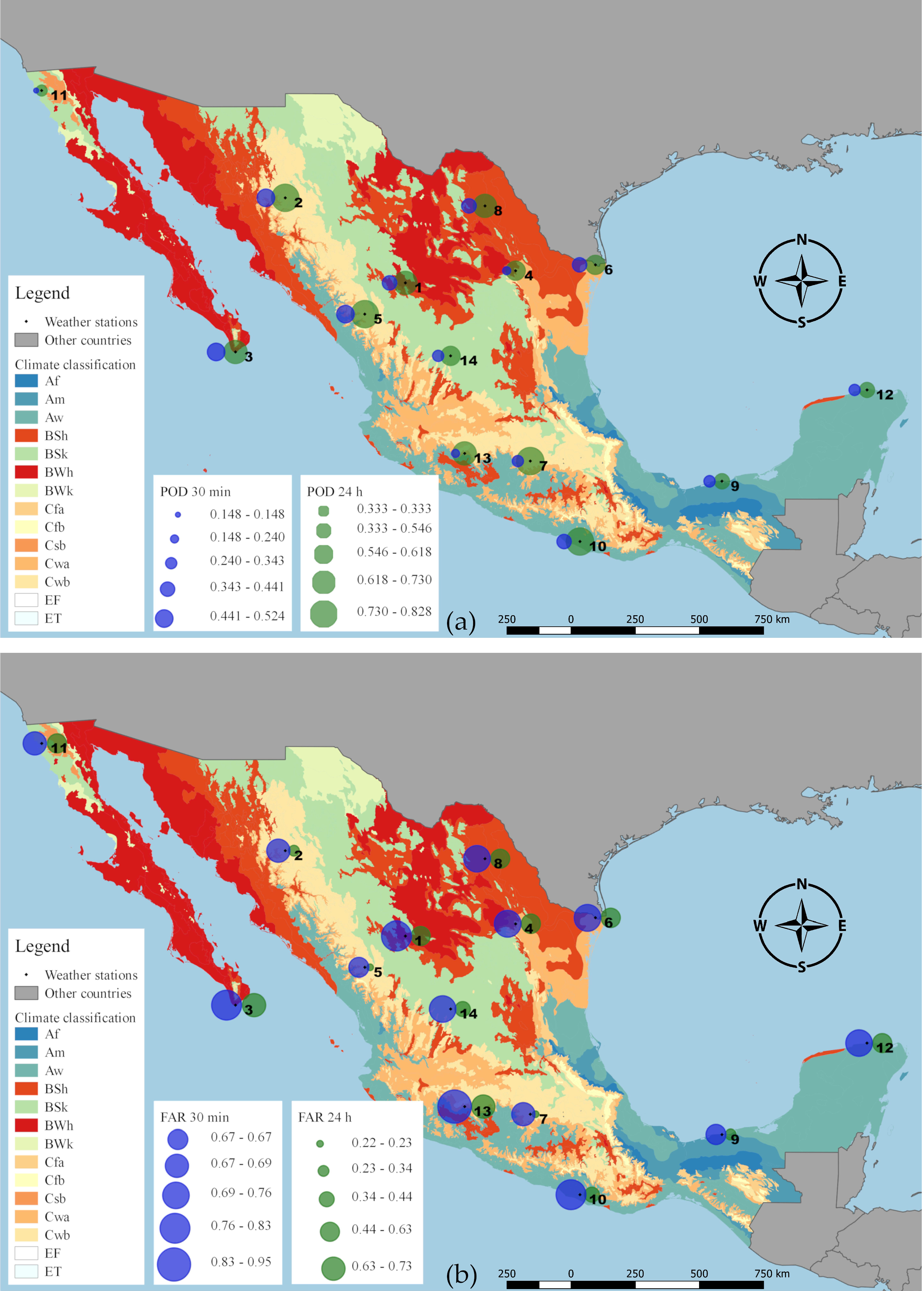
3.1. Analysis of Precipitation Detection Capacity
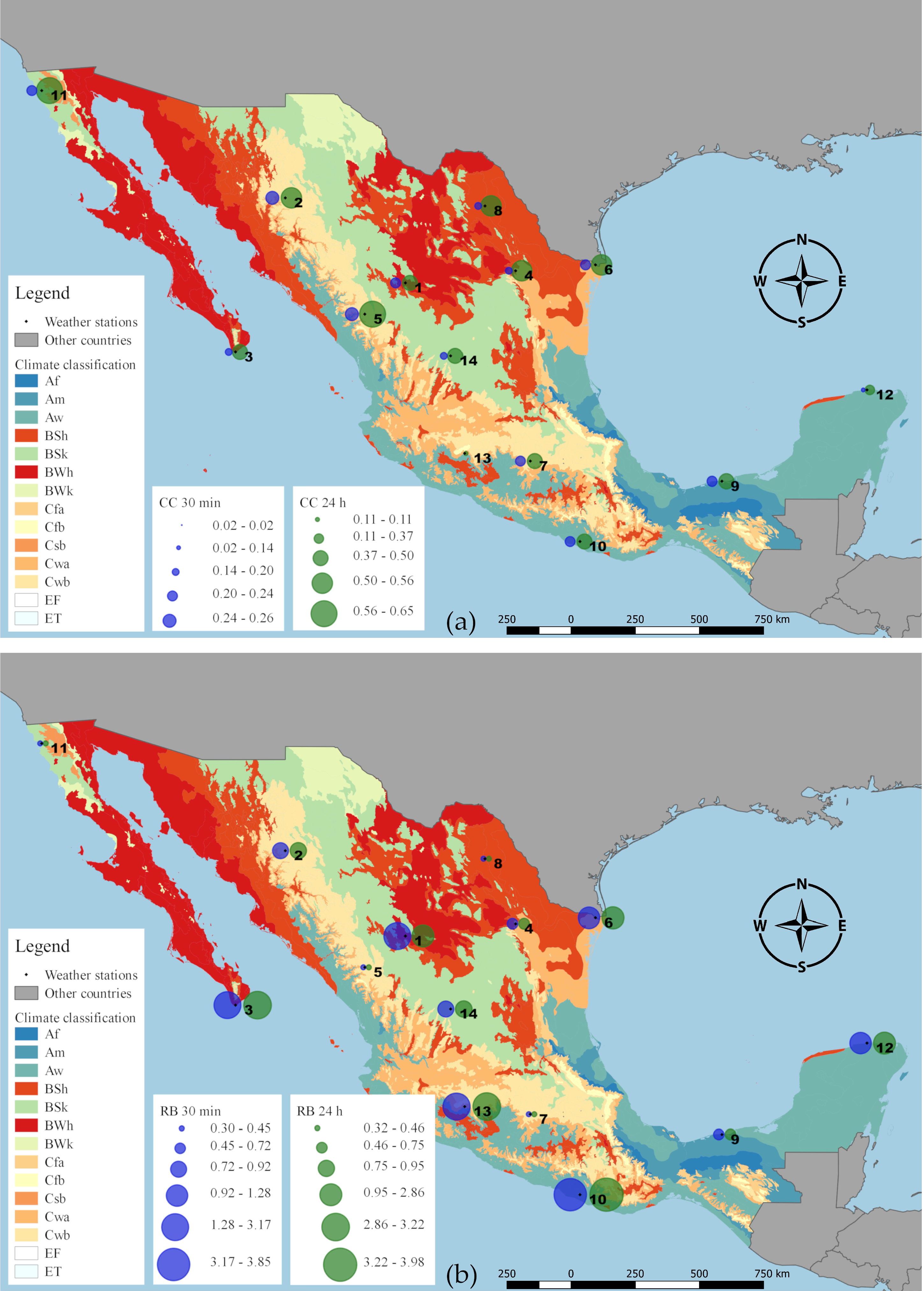
3.2. Quantification of the Precision or Discrepancy between the CMORPH Estimates and the Precipitation Data of the Rain Gauges
4. Discussion
5. Conclusions
- The CMORPH-CRT product has a better performance for the daily aggregation level than for the 30 min level, both in the detection capacity and in the accuracy of the precipitation estimation.
- For the two levels of temporal aggregation, the CMORPH-CRT product overestimates the number of precipitation events, that is, detects more events than actually occurs.
- With respect to the accuracy, for the two levels of temporal aggregation, the CMORPH-CRT product tends to overestimate the amount of precipitation.
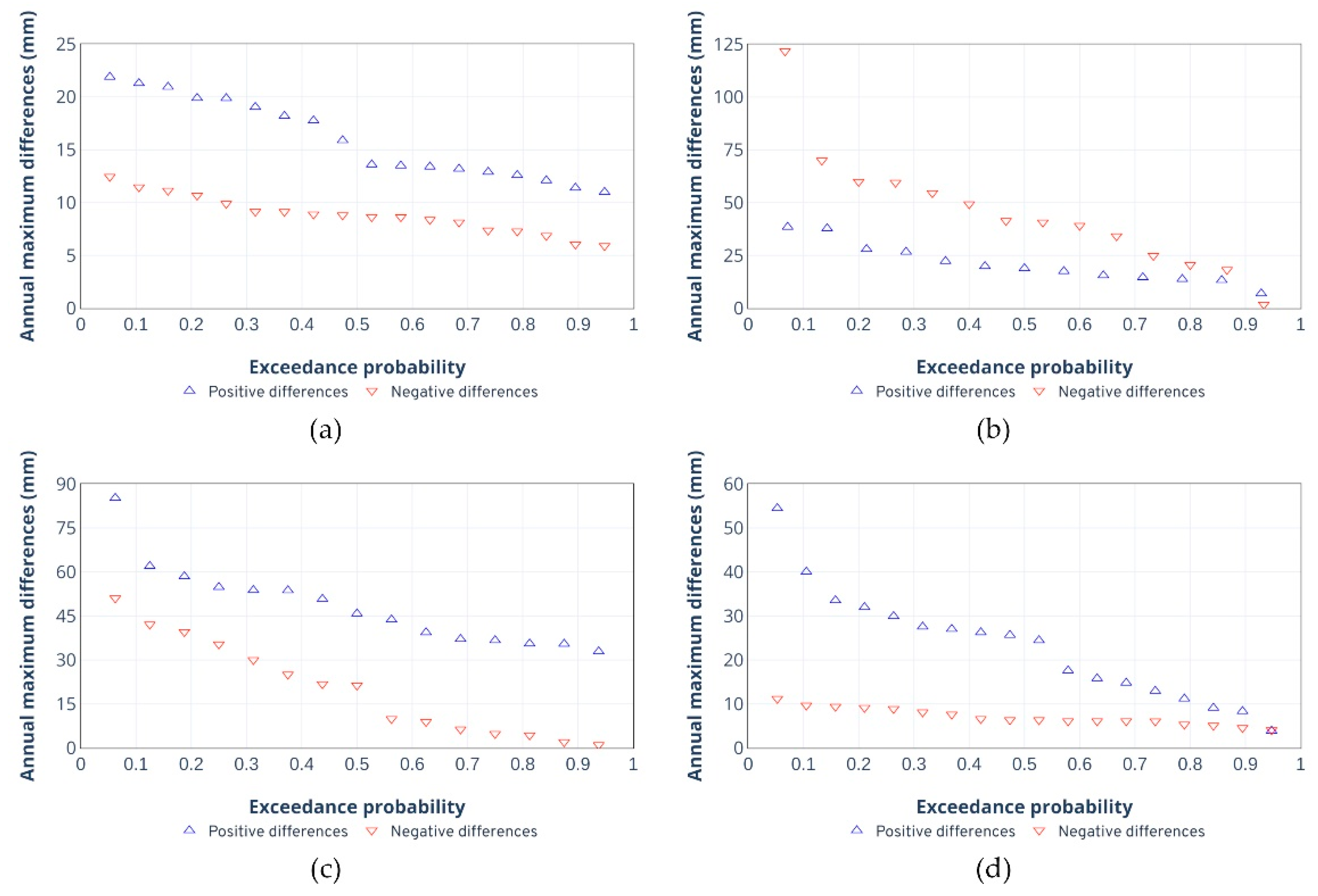
- The results of the analysis of maximum annual differences clearly show the risk of introducing major errors when using the CMORPH-CRT product in hydrological analyzes, research should be conducted focused on identifying the causes of the differences. One of the causes could be the difference in the spatial sampling of the rain gauge and the SBP product since the first provides point measurements and the last delivers spatial averages over the area of a grid cell. The rain gauge may not be detecting convective precipitation events located over the area of the grid cell of the SBP product [16].
Author Contributions
Funding
Acknowledgments
Conflicts of Interest
Appendix A
References
- Alijanian, M.; Rakhshandehroo, G.R.; Mishra, A.K.; Dehghani, M. Evaluation of satellite rainfall climatology using CMORPH, PERSIANN-CDR, PERSIANN, TRMM, MSWEP over Iran. Int. J. Climatol. 2017, 37, 4896–4914. [Google Scholar] [CrossRef]
- Sorooshian, S.; Hsu, K.L.; Gao, X.; Gupta, H.V.; Imam, B.; Braithwaite, D. Evaluation of PERSIANN system satellite-based estimates of tropical rainfall. Bull. Am. Meteorol. Soc. 2000, 81, 2035–2046. [Google Scholar] [CrossRef]
- Joyce, R.J.; Janowiak, J.E.; Arkin, P.A.; Xie, P. CMORPH: A method that produces global precipitation estimates from passive microwave and infrared data at high spatial and temporal resolution. J. Hydrometeorol. 2004, 5, 487–503. [Google Scholar] [CrossRef]
- Huffman, G.J.; Adler, R.F.; Bolvin, D.T.; Gu, G.; Nelkin, E.J.; Bowman, K.P.; Hong, Y.; Stocker, E.F.; Wolff, D.B. The TRMM Multisatellite Precipitation Analysis (TMPA): Quasi-global, multiyear, combined-sensor precipitation estimates at fine scales. J. Hydrometeorol. 2007, 8, 38–55. [Google Scholar] [CrossRef]
- AghaKouchak, A.; Behrangi, A.; Sorooshian, S.; Hsu, K.; Amitai, E. Evaluation of satellite-retrieved extreme precipitation rates across the central United States. J. Geophys. Res. Atmos. 2011, 116, 1–11. [Google Scholar] [CrossRef]
- Jiang, Q.; Li, W.; Wen, J.; Qiu, C.; Sun, W.; Fang, Q.; Xu, M.; Tan, J. Accuracy evaluation of two high-resolution satellite-based rainfall products: TRMM 3B42V7 and CMORPH in Shanghai. Water 2018, 10, 40. [Google Scholar] [CrossRef]
- Kumar, B.; Patra, K.C.; Lakshmi, V. Daily rainfall statistics of TRMM and CMORPH: A case for trans-boundary Gandak river basin. J. Earth Syst. Sci. 2016, 125, 919–934. [Google Scholar] [CrossRef]
- Haile, A.T.; Habib, E.; Rientjes, T. Evaluation of the climate prediction center (CPC) morphing technique (CMORPH) rainfall product on hourly time scales over the source of the Blue Nile River. Hydrol. Process. 2013, 27, 1829–1839. [Google Scholar] [CrossRef]
- Nastos, P.T.; Kapsomenakis, J.; Philandras, K.M. Evaluation of the TRMM 3B43 gridded precipitation estimates over Greece. Atmos. Res. 2016, 169, 497–514. [Google Scholar] [CrossRef]
- Wang, J.; Wolff, D.B. Evaluation of TRMM rain estimates using ground measurements over central Florida. J. Appl. Meteorol. Climatol. 2012, 51, 926–940. [Google Scholar] [CrossRef]
- Quirino, D.T.; Casaroli, D.; Jucá Oliveira, R.A.; Mesquita, M.; Pego Evangelista, A.W.; Alves Júnior, J. Evaluation of TRMM satellite rainfall estimates (algorithms 3B42 V7 & RT) over the Santo Antônio county (Goiás, Brazil). Rev. Fac. Nac. Agron. 2017, 70, 8251–8261. [Google Scholar]
- Ávila-Carrasco, J.R.; Júnez-Ferreira, H.E.; Gowda, P.H.; Steiner, J.L.; Moriasi, D.N.; Starks, P.J.; Gonzalez, J.; Villalobos, A.A.; Bautista-Capetillo, C. Evaluation of satellite-derived rainfall data for multiple physio-climatic regions in the Santiago River Basin, Mexico. J. Am. Water Resour. Assoc. 2018, 54, 1068–1086. [Google Scholar] [CrossRef]
- Xie, P.; Joyce, R.; Wu, S.; Yoo, S.H.; Yarosh, Y.; Sun, F.; Lin, R. Reprocessed, bias-corrected CMORPH global high-resolution precipitation estimates from 1998. J. Hydrometeorol. 2017, 18, 1617–1641. [Google Scholar] [CrossRef]
- Zhang, C.; Chen, X.; Shao, H.; Chen, S.; Liu, T.; Chen, C.; Ding, Q.; Du, H. Evaluation and intercomparison of high-resolution satellite precipitation estimates—GPM, TRMM, and CMORPH in the Tianshan Mountain Area. Remote Sens. 2018, 10, 1543. [Google Scholar] [CrossRef]
- Jiménez-Jiménez, S.I.; Ojeda-Bustamante, W.; Ontiveros-Capurata, R.E.; Flores-Velázquez, J.; de Marcial-Pablo, M.J.; Robles-Rubio, B.D. Quantification of the error of digital terrain models derived from images acquired with UAV. Ing. Agrícola Biosist. 2017, 9, 85–100. [Google Scholar] [CrossRef]
- Cánovas-García, F.; García-Galiano, S.; Alonso-Sarría, F. Assessment of satellite and radar quantitative precipitation estimates for real time monitoring of meteorological extremes over the southeast of the Iberian Peninsula. Remote Sens. 2018, 10, 1023. [Google Scholar] [CrossRef]


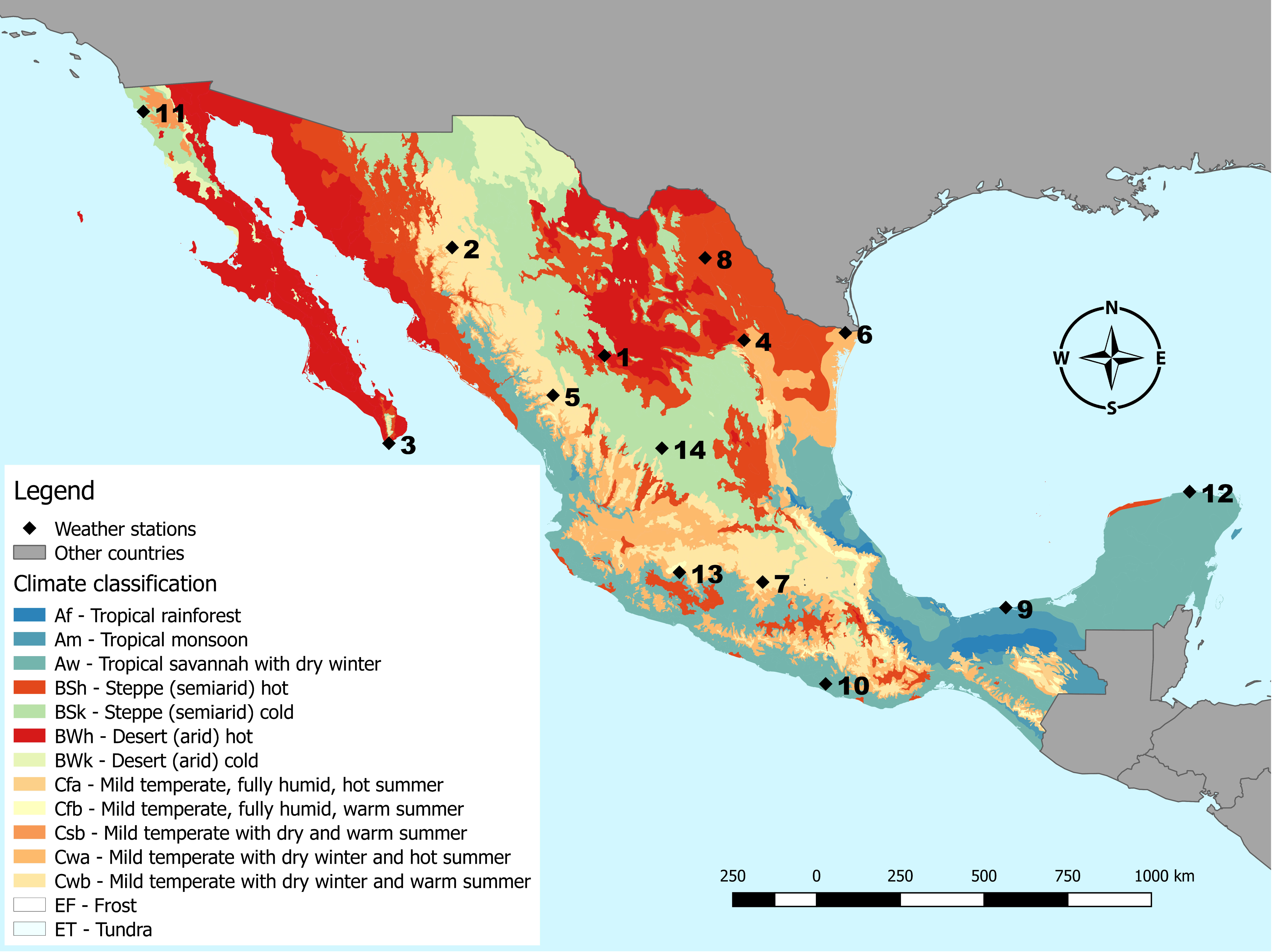
| Station ID | Station Name | State | Municipality | Latitude | Longitude | Altitude Masl | Analysis Period | Climate Code |
|---|---|---|---|---|---|---|---|---|
| 1 | Agustín Melgar | Durango | Nazas | 25.2633 | −104.0661 | 1226 | 2003–2018 | BWh |
| 2 | Basaseachi | Chihuahua | Ocampo | 28.1992 | −108.2089 | 1973 | 2000–2018 | Cwb |
| 3 | Cabo San Lucas | Baja California Sur | Los Cabos | 22.8811 | −109.9264 | 224 | 2000–2018 | BWh |
| 4 | Fierro, N.L. SAHM | Nuevo León | Monterrey | 25.6828 | −100.2719 | 500 | 2001–2017 | BSh |
| 5 | Las Vegas | Durango | San Dimas | 24.1858 | −105.4661 | 2398 | 2003–2018 | Cwb |
| 6 | Matamoros | Tamaulipas | Matamoros | 25.8858 | −97.5186 | 4 | 2000–2018 | Cwa |
| 7 | Nevado de Toluca | México | Toluca | 19.1167 | −99.7667 | 4139 | 2000–2018 | ET |
| 8 | Nueva Rosita | Coahuila | San Juan de Sabinas | 27.9200 | −101.3300 | 366 | 2003–2018 | BSh |
| 9 | Paraíso | Tabasco | Paraíso | 18.4233 | −93.1556 | 4 | 2003–2018 | Am |
| 10 | Pinotepa Nacional | Oaxaca | Santiago Pinotepa Nacional | 16.3497 | −98.0525 | 195 | 2002–2018 | Aw |
| 11 | Presa Emilio López Zamora (Ensenada) | Baja California | Ensenada | 31.8914 | −116.6033 | 32 | 2000–2018 | BSk |
| 12 | Río Lagartos | Yucatán | Río Lagartos | 21.5711 | −88.1603 | 5 | 2000–2018 | Aw |
| 13 | Uruapan | Michoacán | Uruapan | 19.3810 | −102.0291 | 1606 | 1999–2017 | Cwa |
| 14 | Zacatecas | Zacatecas | Guadalupe | 22.7467 | −102.5061 | 2270 | 2000–2018 | BSk |
| CMORPH Algorithm | |||
|---|---|---|---|
| Precipitation Detected | Yes | No | |
| Rain Gauge | Yes | Hit (a) | Miss (c) |
| No | False alarm (b) | Correct negative (d) | |
| Indicator | Range | Optimal Value | Equation | |
|---|---|---|---|---|
| Probability of detection (POD) | [0, 1] | 1 | (1) | |
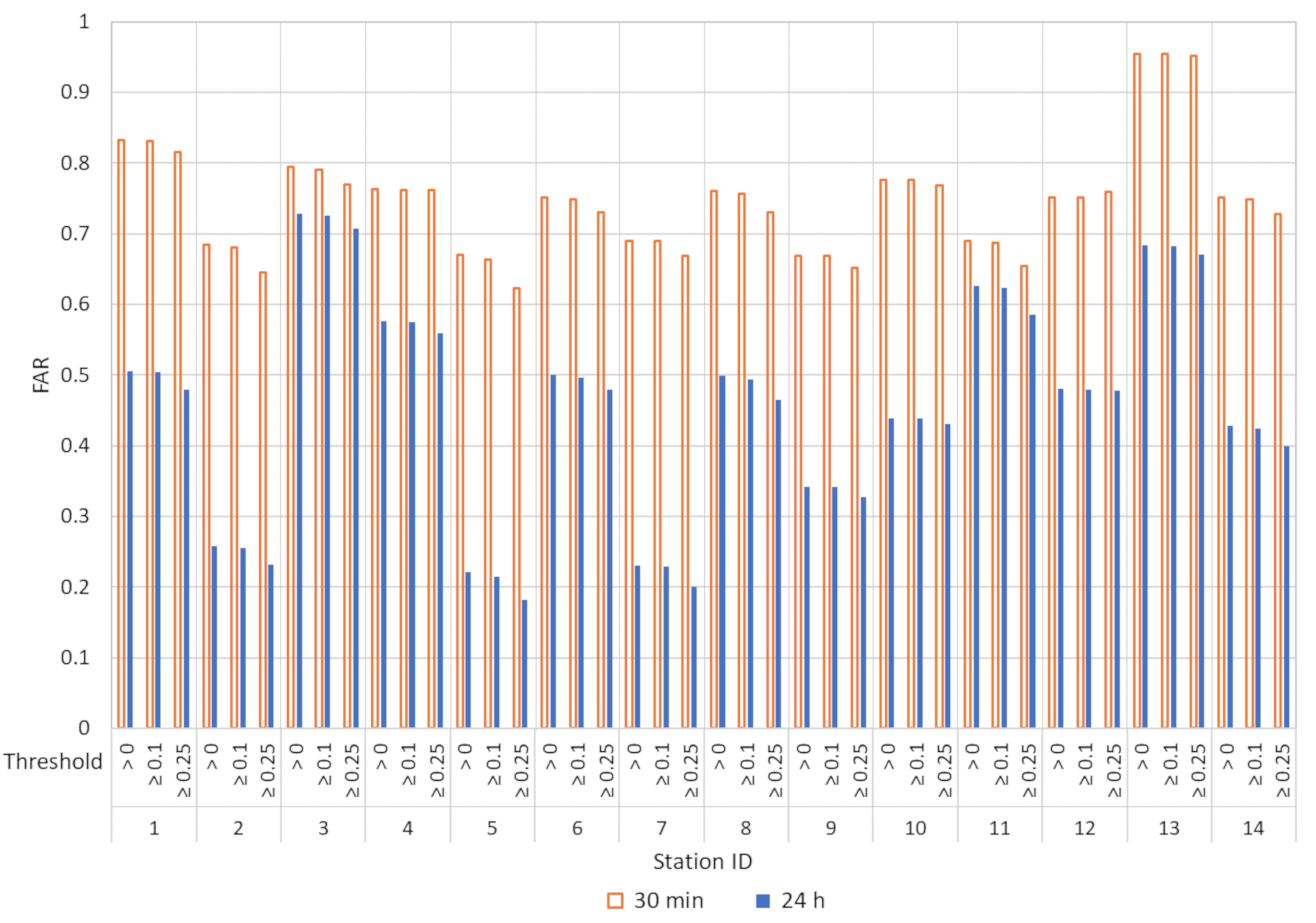
| False alarm rate (FAR) | [0, 1] | 0 | (2) | |
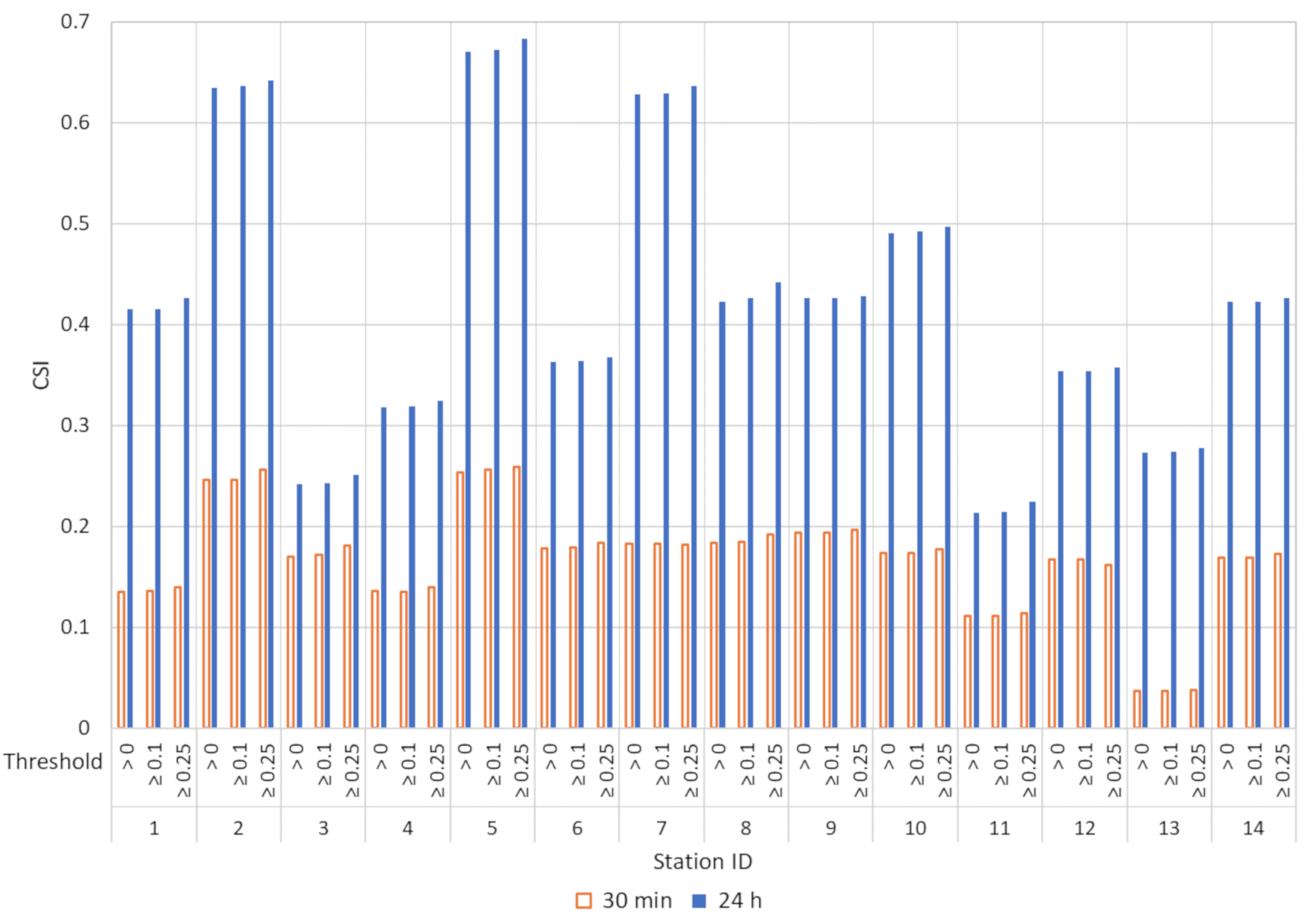
| Critical success index (CSI) | [0, 1] | 1 | (3) | |
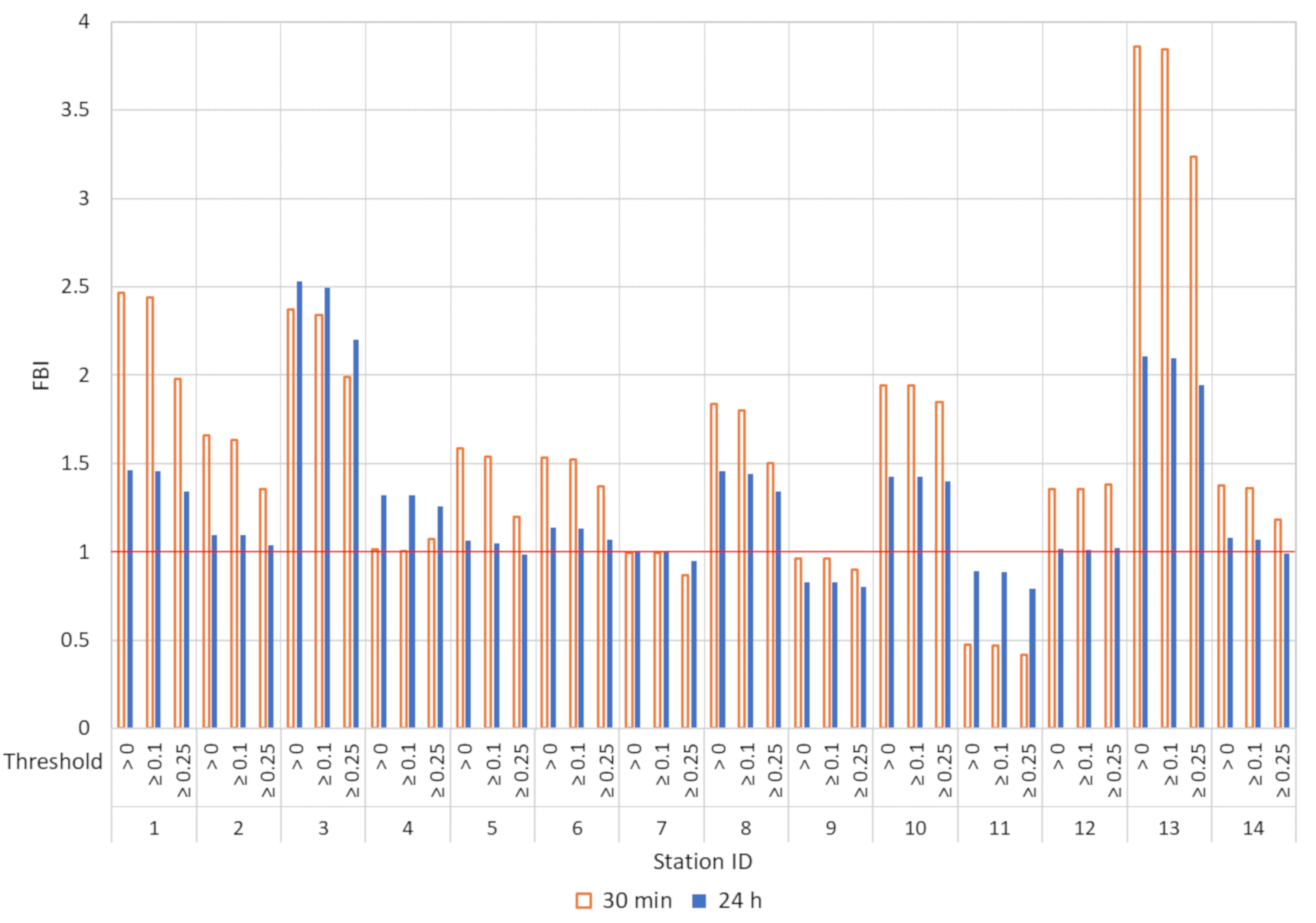
| Frequency bias index (FBI) | [0, ∞] | 1 | (4) | |
| Indicator | Range | Optimal Value | Equation | |
|---|---|---|---|---|
| Mean absolute error (MAE) | [0, ∞] | 0 | (5) | |
| Root of the mean square error (RMSE) | [0, ∞] | 0 | (6) | |
| Relative bias (RB) | [−∞, ∞] | 0 | (7) | |
| Correlation coefficient (CC) | [−1, 1] | 1 | (8) | |
| Station ID | Indicator | |||||||||||
|---|---|---|---|---|---|---|---|---|---|---|---|---|
| POD | FAR | |||||||||||
| Temporal Aggregation Level | Temporal Aggregation Level | |||||||||||
| 30 | 30 | 30 | 24 | 24 | 24 | 30 | 30 | 30 | 24 | 24 | 24 | |
| (min) | (min) | (min) | (h) | (h) | (h) | (min) | (min) | (min) | (h) | (h) | (h) | |
| Threshold | Threshold | Threshold | Threshold | |||||||||
| >0 | ≥0.1 | ≥0.25 | >0 | ≥0.1 | ≥0.25 | >0 | ≥0.1 | ≥0.25 | >0 | ≥0.1 | ≥0.25 | |
| 1 | 0.413 | 0.412 | 0.366 | 0.722 | 0.722 | 0.700 | 0.832 | 0.831 | 0.815 | 0.506 | 0.505 | 0.479 |
| 2 | 0.524 | 0.520 | 0.480 | 0.814 | 0.814 | 0.797 | 0.684 | 0.681 | 0.645 | 0.258 | 0.256 | 0.232 |
| 3 | 0.490 | 0.490 | 0.458 | 0.689 | 0.684 | 0.643 | 0.794 | 0.791 | 0.770 | 0.728 | 0.726 | 0.708 |
| 4 | 0.240 | 0.239 | 0.255 | 0.561 | 0.561 | 0.555 | 0.763 | 0.762 | 0.762 | 0.576 | 0.575 | 0.559 |
| 5 | 0.522 | 0.518 | 0.451 | 0.828 | 0.823 | 0.805 | 0.670 | 0.663 | 0.623 | 0.221 | 0.215 | 0.182 |
| 6 | 0.383 | 0.382 | 0.368 | 0.569 | 0.569 | 0.556 | 0.751 | 0.749 | 0.731 | 0.500 | 0.497 | 0.479 |
| 7 | 0.309 | 0.309 | 0.287 | 0.774 | 0.774 | 0.758 | 0.690 | 0.690 | 0.669 | 0.231 | 0.229 | 0.201 |
| 8 | 0.441 | 0.437 | 0.403 | 0.730 | 0.728 | 0.716 | 0.760 | 0.757 | 0.731 | 0.499 | 0.494 | 0.465 |
| 9 | 0.318 | 0.318 | 0.312 | 0.547 | 0.547 | 0.541 | 0.669 | 0.669 | 0.652 | 0.342 | 0.342 | 0.328 |
| 10 | 0.436 | 0.436 | 0.427 | 0.799 | 0.799 | 0.796 | 0.776 | 0.776 | 0.768 | 0.439 | 0.439 | 0.431 |
| 11 | 0.148 | 0.148 | 0.145 | 0.333 | 0.333 | 0.329 | 0.690 | 0.687 | 0.654 | 0.626 | 0.624 | 0.585 |
| 12 | 0.337 | 0.337 | 0.333 | 0.528 | 0.526 | 0.533 | 0.751 | 0.751 | 0.759 | 0.481 | 0.480 | 0.478 |
| 13 | 0.174 | 0.174 | 0.154 | 0.665 | 0.665 | 0.641 | 0.955 | 0.955 | 0.952 | 0.684 | 0.683 | 0.671 |
| 14 | 0.342 | 0.341 | 0.322 | 0.618 | 0.616 | 0.595 | 0.751 | 0.749 | 0.728 | 0.428 | 0.425 | 0.400 |
| Mean | 0.363 | 0.362 | 0.340 | 0.656 | 0.654 | 0.640 | 0.753 | 0.751 | 0.733 | 0.466 | 0.464 | 0.443 |
| SD | 0.119 | 0.118 | 0.105 | 0.139 | 0.138 | 0.134 | 0.076 | 0.077 | 0.086 | 0.160 | 0.161 | 0.163 |
| Station ID | Indicator | |||||||||||
|---|---|---|---|---|---|---|---|---|---|---|---|---|
| CSI | FBI | |||||||||||
| Temporal Aggregation Level | Temporal Aggregation Level | |||||||||||
| 30 | 30 | 30 | 24 | 24 | 24 | 30 | 30 | 30 | 24 | 24 | 24 | |
| (min) | (min) | (min) | (h) | (h) | (h) | (min) | (min) | (min) | (h) | (h) | (h) | |
| Threshold | Threshold | Threshold | Threshold | |||||||||
| >0 | ≥0.1 | ≥0.25 | >0 | ≥0.1 | ≥0.25 | >0 | ≥0.1 | ≥0.25 | >0 | ≥0.1 | ≥0.25 | |
| 1 | 0.135 | 0.136 | 0.140 | 0.415 | 0.415 | 0.426 | 2.463 | 2.440 | 1.978 | 1.461 | 1.459 | 1.344 |
| 2 | 0.246 | 0.246 | 0.256 | 0.635 | 0.636 | 0.642 | 1.633 | 1.633 | 1.353 | 1.096 | 1.094 | 1.038 |
| 3 | 0.170 | 0.172 | 0.181 | 0.242 | 0.243 | 0.251 | 2.372 | 2.341 | 1.991 | 2.533 | 2.495 | 2.200 |
| 4 | 0.136 | 0.135 | 0.140 | 0.318 | 0.319 | 0.325 | 1.012 | 1.005 | 1.071 | 1.322 | 1.320 | 1.259 |
| 5 | 0.254 | 0.256 | 0.259 | 0.670 | 0.672 | 0.683 | 1.583 | 1.537 | 1.197 | 1.063 | 1.047 | 0.985 |
| 6 | 0.178 | 0.179 | 0.184 | 0.363 | 0.364 | 0.368 | 1.535 | 1.522 | 1.368 | 1.137 | 1.131 | 1.067 |
| 7 | 0.183 | 0.183 | 0.182 | 0.628 | 0.629 | 0.636 | 0.995 | 0.994 | 0.867 | 1.007 | 1.004 | 0.948 |
| 8 | 0.184 | 0.185 | 0.192 | 0.423 | 0.426 | 0.442 | 1.838 | 1.798 | 1.499 | 1.456 | 1.439 | 1.339 |
| 9 | 0.194 | 0.194 | 0.197 | 0.426 | 0.426 | 0.428 | 0.961 | 0.961 | 0.899 | 0.830 | 0.830 | 0.804 |
| 10 | 0.174 | 0.174 | 0.177 | 0.491 | 0.492 | 0.497 | 1.944 | 1.943 | 1.845 | 1.425 | 1.424 | 1.398 |
| 11 | 0.111 | 0.111 | 0.114 | 0.214 | 0.215 | 0.225 | 0.476 | 0.471 | 0.418 | 0.892 | 0.886 | 0.793 |
| 12 | 0.167 | 0.167 | 0.162 | 0.354 | 0.354 | 0.358 | 1.356 | 1.354 | 1.381 | 1.017 | 1.012 | 1.020 |
| 13 | 0.037 | 0.037 | 0.038 | 0.273 | 0.274 | 0.278 | 3.857 | 3.846 | 3.234 | 2.105 | 2.096 | 1.946 |
| 14 | 0.169 | 0.169 | 0.173 | 0.423 | 0.423 | 0.426 | 1.374 | 1.360 | 1.184 | 1.080 | 1.071 | 0.992 |
| Mean | 0.167 | 0.167 | 0.171 | 0.420 | 0.421 | 0.428 | 1.673 | 1.658 | 1.449 | 1.316 | 1.308 | 1.224 |
| SD | 0.054 | 0.054 | 0.055 | 0.144 | 0.145 | 0.145 | 0.834 | 0.829 | 0.675 | 0.477 | 0.470 | 0.410 |
| Station ID | MAE | RMSE | RB | CC | ||||
|---|---|---|---|---|---|---|---|---|
| 30 min | 24 h | 30 min | 24 h | 30 min | 24 h | 30 min | 24 h | |
| 1 | 0.048 | 1.825 | 0.445 | 7.524 | 2.616 | 2.856 | 0.219 | 0.466 |
| 2 | 0.121 | 4.065 | 0.748 | 11.173 | 0.921 | 0.951 | 0.250 | 0.529 |
| 3 | 0.025 | 0.969 | 0.467 | 9.411 | 2.816 | 3.223 | 0.168 | 0.464 |
| 4 | 0.091 | 3.021 | 0.750 | 10.866 | 0.721 | 0.746 | 0.197 | 0.546 |
| 5 | 0.085 | 2.391 | 0.557 | 6.599 | 0.299 | 0.323 | 0.260 | 0.608 |
| 6 | 0.087 | 3.070 | 0.890 | 13.854 | 1.279 | 1.386 | 0.237 | 0.563 |
| 7 | 0.134 | 4.171 | 0.629 | 9.299 | 0.424 | 0.420 | 0.233 | 0.477 |
| 8 | 0.084 | 2.735 | 0.970 | 11.284 | 0.448 | 0.458 | 0.166 | 0.532 |
| 9 | 0.183 | 6.802 | 1.398 | 25.500 | 0.578 | 0.650 | 0.213 | 0.495 |
| 10 | 0.219 | 9.213 | 1.545 | 26.448 | 3.854 | 3.983 | 0.218 | 0.495 |
| 11 | 0.026 | 0.960 | 0.423 | 5.790 | 0.401 | 0.416 | 0.234 | 0.652 |
| 12 | 0.097 | 3.684 | 1.077 | 17.460 | 1.154 | 1.222 | 0.139 | 0.367 |
| 13 | 0.125 | 5.234 | 0.730 | 12.546 | 3.173 | 3.199 | 0.018 | 0.111 |
| 14 | 0.059 | 2.121 | 0.557 | 7.718 | 0.893 | 0.903 | 0.193 | 0.471 |
© 2019 by the authors. Licensee MDPI, Basel, Switzerland. This article is an open access article distributed under the terms and conditions of the Creative Commons Attribution (CC BY) license (http://creativecommons.org/licenses/by/4.0/).
Share and Cite
Bruster-Flores, J.L.; Ortiz-Gómez, R.; Ferriño-Fierro, A.L.; Guerra-Cobián, V.H.; Burgos-Flores, D.; Lizárraga-Mendiola, L.G. Evaluation of Precipitation Estimates CMORPH-CRT on Regions of Mexico with Different Climates. Water 2019, 11, 1722. https://doi.org/10.3390/w11081722
Bruster-Flores JL, Ortiz-Gómez R, Ferriño-Fierro AL, Guerra-Cobián VH, Burgos-Flores D, Lizárraga-Mendiola LG. Evaluation of Precipitation Estimates CMORPH-CRT on Regions of Mexico with Different Climates. Water. 2019; 11(8):1722. https://doi.org/10.3390/w11081722
Chicago/Turabian StyleBruster-Flores, José L., Ruperto Ortiz-Gómez, Adrian L. Ferriño-Fierro, Víctor H. Guerra-Cobián, Dagoberto Burgos-Flores, and Liliana G. Lizárraga-Mendiola. 2019. "Evaluation of Precipitation Estimates CMORPH-CRT on Regions of Mexico with Different Climates" Water 11, no. 8: 1722. https://doi.org/10.3390/w11081722