Article

Effect of Sediment Load Boundary Conditions in Predicting Sediment Delta of Tarbela Reservoir in Pakistan

by
Zeeshan Riaz Tarar
1,
Sajid Rashid Ahmad
1,
Iftikhar Ahmad
1,
Shabeh ul Hasson
2,3,
Zahid Mahmood Khan
4,
Rana Muhammad Ali Washakh
5,6,
Sardar Ateeq-Ur-Rehman
4,7,* and
Minh Duc Bui
7
1
College of Earth & Environmental Sciences (CEES), University of the Punjab, Punjab 54590, Pakistan
2
CEN, Institute of Geography, University of Hamburg, 20148 Hamburg, Germany
3
Department of Space Science, Institute of Space Technology, Islamabad 44000, Pakistan
4
Department of Agriculture Engineering, BZ University, Multan 60800, Pakistan
5
Key Laboratory of Mountain Hazards and Surface Process, Institute of Mountain Hazards and Environment, Chinese Academy of Sciences, Chengdu 610041, China
6
University of Chinese Academy of Sciences, Beijing 100049, China
7
Chair of Hydraulic and Water Resources Engineering, Technical University of Munich, 80333 Munich, Germany
*
Author to whom correspondence should be addressed.
Water 2019, 11(8), 1716; https://doi.org/10.3390/w11081716
Submission received: 16 June 2019 / Revised: 10 August 2019 / Accepted: 13 August 2019 / Published: 18 August 2019
(This article belongs to the Special Issue Modeling of Soil Erosion and Sediment Transport)

Abstract

:
Setting precise sediment load boundary conditions plays a central role in robust modeling of sedimentation in reservoirs. In the presented study, we modeled sediment transport in Tarbela Reservoir using sediment rating curves (SRC) and wavelet artificial neural networks (WA-ANNs) for setting sediment load boundary conditions in the HEC-RAS 1D numerical model. The reconstruction performance of SRC for finding the missing sediment sampling data was at R2 = 0.655 and NSE = 0.635. The same performance using WA-ANNs was at R2 = 0.771 and NSE = 0.771. As the WA-ANNs have better ability to model non-linear sediment transport behavior in the Upper Indus River, the reconstructed missing suspended sediment load data were more accurate. Therefore, using more accurately-reconstructed sediment load boundary conditions in HEC-RAS, the model was better morphodynamically calibrated with R2 = 0.980 and NSE = 0.979. Using SRC-based sediment load boundary conditions, the HEC-RAS model was calibrated with R2 = 0.959 and NSE = 0.943. Both models validated the delta movement in the Tarbela Reservoir with R2 = 0.968, NSE = 0.959 and R2 = 0.950, NSE = 0.893 using WA-ANN and SRC estimates, respectively. Unlike SRC, WA-ANN-based boundary conditions provided stable simulations in HEC-RAS. In addition, WA-ANN-predicted sediment load also suggested a decrease in supply of sediment significantly to the Tarbela Reservoir in the future due to intra-annual shifting of flows from summer to pre- and post-winter. Therefore, our future predictions also suggested the stability of the sediment delta. As the WA-ANN-based sediment load boundary conditions precisely represented the physics of sediment transport, the modeling concept could very likely be used to study bed level changes in reservoirs/rivers elsewhere in the world.

1. Introduction

The uncertainties in modeling reservoir sedimentation are due to: (a) both flow and sediment; (b) the distribution of sediment particle size; (c) the specific weights of sediment deposits; (d) reservoir geometry; and (e) the operational rules of reservoirs [1]. These uncertainties are propagated, particularly, due to the varying input of sediment loads as boundary conditions. Normally, sediment series, as input to the model, are estimated by utilizing sediment rating curves (SRCs), prepared by developing relationships through simple regression techniques, between flow and sediment, observed over a considerable period, adequately representing the complete hydrological cycle over decades [2,3]. It has been observed in various sediment studies of reservoirs around the world that SRCs, though a simple and convenient way to estimate missing values of sediment inflow, often overestimate and overshoot the sediment entry into the reservoirs against the actual conditions, up to 50% [4,5]. Tarbela Reservoir hydrographical/bathymetric surveys have been conducted since 1979 to observe the sediment entry and position/advancement of the delta in the reservoir. Each year, the reservoir authorities issue Sedimentation Reports based on the above conducted surveys. As per the Sedimentation Report of Tarbela Reservoir [6], the actual observed sediment deposits in the reservoir are about 171.3 Mt/year, which are about 53% of the average of the below-mentioned studies, i.e., 47% overestimation. Hence, precise hydro-morphodynamic boundary conditions play a principal role in modeling the transport processes in rivers and reservoirs.
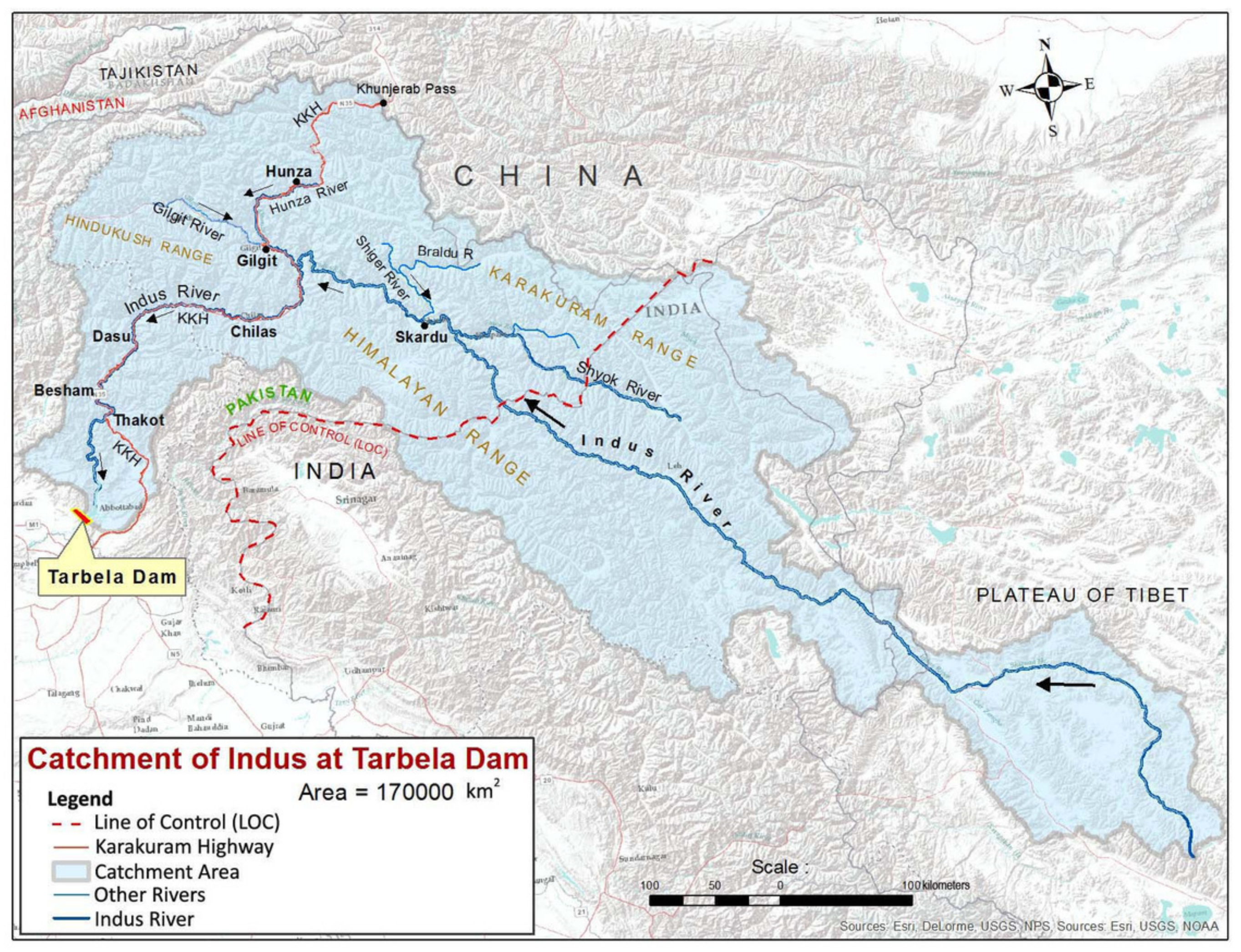
The Tarbela Dam Project (TDP) was completed in the mid-1970s and is the backbone of the hydropower and water resources of Pakistan, with its 3478 MW of existing installed and 6298 MW of near future capacity. It is the world’s largest earth-filled dam and also by structural volume [7]. The Tarbela Reservoir drains UIB and lies at its lowest point. The drainage area up to the dam is about 170,000 km2, as shown and demarcated in Figure 1. The huge body of water created behind the dam, originally 11.620 million acre feet (MAF), has been reduced by sedimentation to 6.856 MAF in 2019 [8], meaning that it is only 59% of its original storage volume, and the rest has been consumed by sedimentation. The feasibility and engineering studies of Tarbela Dam that were conducted in the mid-1960s and 1970s took serious note of the potential sedimentation problems that were likely to arise after some years of dam construction. Various studies at the time and afterwards estimated sediment entering the reservoir to be substantially overestimated, based primarily on techniques in vogue and with less data. The Tarbela Dam Consultants (Tippets, Abbett, McCarthy, Stratton (TAMS)) used 235 million tons (Mt) annually as the sediments entering the reservoir [9]. The Kalabagh Dam Consultants estimated the annual sediment load entering Tarbela as 295.7 Mt using sediment rating curves. The same figure of 295.7 Mt was adopted for sediment studies of Tarbela by the Consultants of the Ghazi Barotha Hydropower Project located just 8 km downstream of Tarbela Dam. The Consultants for the Mega Diamer-Basha Dam, making use of additional data from 1962–2003 in sediment rating curves, calculated the load for Tarbela Reservoir as 233 Mt annually [10]. Future sedimentation scenarios fir Tarbela Reservoir hold a pivotal position for authorities and water managers alike, as a reduction in the storage capacity of Pakistan’s largest water body and its implications for all related disciplines would be sensitive enough to provoke studies into alternative or preventive measures.
A list of studies also cited by [11], in addition to the ones mentioned above, calculating sediment entering Tarbela Reservoir/main Upper Indus Basin (UIB), is tabulated in Table 1:
All above estimates were based on sediment rating curve (SRC) method and varied in a wide range from around 200 Mt y−1 – 675 Mt y−1 over the last 50 years. Unfortunately, the accuracy of SRCs is limited, as they map all scattered data points of discharge and sediment loads using a single fitting line, which is more likely to be affected by data outliers [22,23,24]. Therefore, the single fitting line cannot handle sediment transport processes connected to the phenomenon of hysteresis and noticeable hydrological variations, such as: (a) fluvial erosion and transport processes, interacting with other sediment-production processes; (b) sediment temporary storage in the main channel of the river [25]; (c) landslide phases related to aggradation and degradation [26]; (d) on average, 5–10 waves of high flow of an average of 10–12 days’ duration during the monsoon period; (e) different discharge and sediment conveyance times and their differing lag-times from sources to the gauge recording stations. Basically, all these processes cause different sediment concentrations on same magnitude of discharge during rising and falling limbs of flood events, which is referred to as the hysteresis phenomenon. As SRCs are mostly employed in the estimation process of sediment load boundary conditions due to their construction simplicity, a marked compromise could arise in the numerical or physical modeling outcomes.
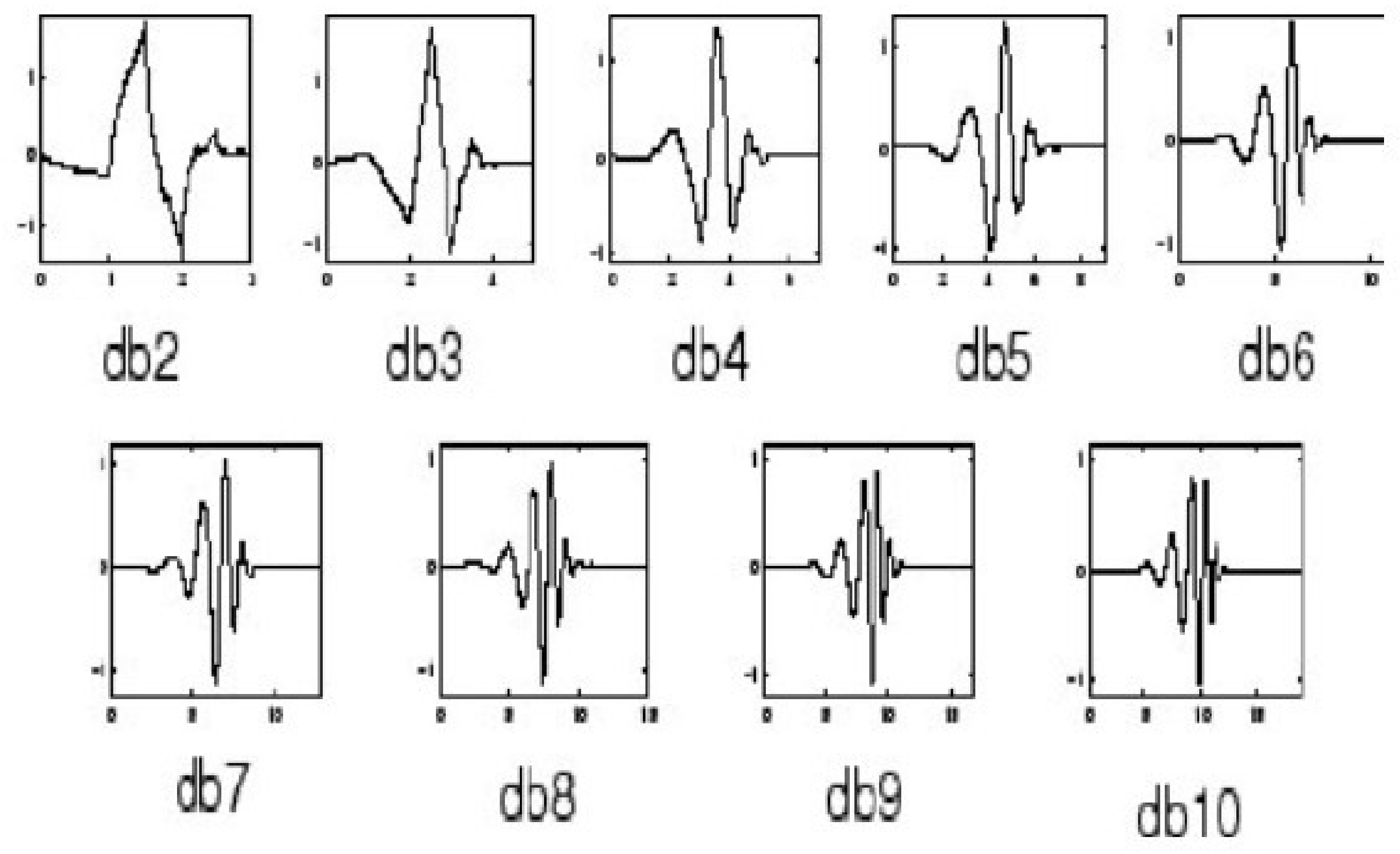
Since the variations in sediment load boundary conditions affect the calculations of the morphodynamics, it is essential to model time-related changes in sediment supply more accurately, influenced by the above-mentioned phenomenon of hysteresis and noticeable hydrological changes. During recent years, artificial neural networks (ANNs) have gained increased reception as new analytical techniques due to their robustness and ability to model non-stationary data series. Therefore, ANNs have a clear advantage over other conceptual models as they do not need previous knowledge of the process because they build a relationship between data inputs and targets using non-linear activation functions. The ANNs have multiple inputs with dissimilar characteristics, making ANNs be able to represent time-space variation [1]. In spite of the adequate flexibility of ANNs in modeling time series, sometimes, ANNs have a weakness when signal alterations are highly non-stationary and physical hydrological processes operate under scales of large ranges, with variations of one day to several years. In such a situation, different methods have been proposed, among which are wavelet transforms. They have become a capable method for analyzing such changes and trends in hydrological time series [27,28,29,30,31]. A wavelet has been defined as a small wave whose energy is limited in a short period of time and is a logical method for signals that are non-stationary, having short-lived transient components, featuring at different scales, or singularities. A non-stationary signal can be broken up into a certain number of unvarying signals by wavelet transform. ANN is then combined with wavelet transform (WA-ANN). It is considered that WA-ANN models are more precise than the conventional methods since wavelet transforms provide effective break-ups of the original time series, and the wavelet transformation data improves the performance of conventional ANN models by catching effective information for various resolution levels [4,5,11].
In the present study, effort has been made to model the sediment delta of Tarbela Reservoir using the 1D HEC-RAS numerical model with the objective to reduce variations in its future prediction by employing first the conventionally-estimated sediment inflow based on SRC and then by the above elaborated innovative WA-ANN technique. The sediment series based on WA-ANN, as developed by [4,11], was further updated, calibrated, and validated by inclusion of sediment data up to 2014 and used as input to the model.

2. Methods

2.1. HEC-RAS Program System

The River Analysis System (HEC-RAS), a one-dimensional model, created by Hydrologic Engineering Centre, has been designed to carry out steady flow water surface profile computations of natural rivers and networks of natural and constructed channels, unsteady flow simulations, moving boundary sediment transport computations, and water quality analysis. All these components utilize a common geometric data representation and hydraulic computation procedures. The calculations of one-dimensional moving material of the river bed causing scour or deposition over a certain modeling period establish a base for sediment transport simulations. Generally, sediment transport in rivers, channels, and streams depends on two modes: bed load and suspended load, which in turn depend on sediment particle size, the velocity of water, and river bed slope. The basic idea of evaluating sediment transport capacity by HEC-RAS is by computing sediment capacity of each cross-section as a control volume and for all particle sizes. HEC-RAS requires boundary condition data of each type for making such calculations. The boundary conditions are necessary to get the solution to the differential equations set, describing the problem over the area of interest. There are a number of boundary conditions for steady flow and sediment analysis computations in HEC-RAS. Boundary conditions can be either external, which are specified at the ends of the simulated network at the upstream/downstream, or internal, which are to be used for connecting junctions. Background information regarding computational methods and equations used in modeling sediment transport is available in [32].

2.2. Data Collection

Owing to the noticeable global warming influence on the hydrological and river systems observed around the turn of the century, we considered to start the modeling process from 2005 onward [33,34,35,36,37,38]. For this, we collected the levels of Tarbela Reservoir and the flows of the Indus River at Besham Qila, the nearest station to the upper periphery of the reservoir located about 134 km upstream of the dam, from the project authorities for the 2005–2018 period. To hydrodynamically and morphodynamically initialize, calibrate, and validate the model, bathymetric surveys of the Tarbela Reservoir for the years 2005, 2013, and 2017 were also obtained.
To develop SRC and WA-ANN models, suspended sediment concentrations (ppm) and its gradational data at Besham Qila gauge recording station were collected for the 1969–2014 period from the Surface Water Hydrology Project (SWHP) of the Water and Power Development Authority (WAPDA), Pakistan. The raw data so collected are presented in Figure 2.
The Tarbela Reservoir was cut into 73 cross-sections or range lines (R/Lines) to study the morphodynamics of the huge reservoir (see Figure 3).
The first comprehensive reservoir survey after the dam’s construction was in 1974, and since then, each year, hydro-graphic surveys of the Tarbela Reservoir have been conducted. To cover the whole reservoir area, i.e., 161 km2, the hydro-graphic surveys were conducted using a systematic sounding method over the 73 cross-sectional range lines. Approximately 3500–4000 sounding measurements of the bed level alterations, reservoir depths, and water level elevations along these range lines are available, which were collected mostly during September–November. The distance between the cross-sections/range lines and the measured data points along these cross-sections are not identical. The average distance between each cross-section measured along River Thalweg was approximately 1000 m. However, compared to the upper periphery of the reservoir, the distances between the cross-sections nearer to the dam were smaller. The distance between measured data points along the cross-sections, i.e., lateral distance in y direction, was also variable with a mean of 39 m. The mean cross-sectional width near the dam axis was approximately 4000–5000 m, reducing to only 90–150 m near the upper periphery of the reservoir. Therefore, the major storage volume is near the dam axis, containing huge sediment deposits.
Water depths in the reservoir vary from a maximum 150 m near the dam to mostly 20 m at the reservoir inlet. To secure the stability of the dam and bank slopes along the reservoir, the maximum lowering and rising rate for the reservoir during operation is 4 m/day and 3 m/day, respectively, between reservoir levels 396 and 460 m and only 1 m/day up to the maximum conservation level of 472.5 m asl. The average slope of the river bed in 1979 was 0.0011211, which decreased in 2010 with an average slope of 0.0005988.

2.3. Performance Measures for Model Evaluation

To assess the performance of the models in terms of accuracy and consistency in simulating reservoir water depths and river bed levels, the following three statistical measures tests were made up of: (a) the coefficient of determination (R2), an indication of the level of the relationship between the observed and simulated data, ranging from 0–1; (b) the observations’ standard deviation ratio (RSR), the ratio of the root mean squared error (RMSE) to the standard deviation (STDEV) of the observed data; (c) the Nash–Sutcliffe efficiency (NSE), a statistical assessment to calculate the relative magnitude of residual variance compared to the measured data variance [39]. The formulas are shown in Table 2.

2.4. Sediment Rating Curves

The SRC method is based on an empirical relationship between the discharge and the sediment concentration/load. Likewise, the collected suspended sediment concentration samples were converted into suspended sediment load (SSL) in t/day and related to their corresponding discharges in m3/s to develop the rating curves, encompassing low and high flow conditions. Additionally, 10% bed load was added to the suspended load as recommended by [10]. Total load equations (Equations (1) and (2)) are expressed in the form QT = a Qb, where QT is sediment discharge in t/day; Q is water discharge in m3/s; and a and b are constants as solved on page 15 of [3]. They were entered as upper boundary conditions in the model and depicted graphically in Figure 4.
Q T = 1 . 686 × 10 4 Q 2 . 627 , for Q > = 481 m 3 / s
Q T = 4 . 474 × 10 32 Q 12 . 868 , for Q < 481 m 3 / s
where Q T = total load (suspended + bed load) in t/day with respect to flow discharge Q in m3/s.
The annual load calculated by SRC was 212 million tons (Mt). The calculated monthly loads are shown in Table 3 and Figure 5. As can be seen, most of the sediment transport processes took place in the summer months. Against 84% of the annual flow, 98% of the sediment load transport occurred from May–September.

2.5. Wavelet-Artificial Neural Network

2.5.1. Wavelet Transform

Recently, wavelet analysis has been widely accepted in a wide range of science and engineering applications. Some of the latest studies utilizing the wavelet analysis are [4,27,28,29,30,31]. The wavelet analysis technique has also been used in: data and image compression, partial differential equation solving, transient detection, pattern recognition, texture analysis, noise reduction, trend detection, etc. Wavelets have been identified as more effective tools than the Fourier transform (FT) in analyzing the non-stationary time series. Instead of FT, which analyses the data in two dimensions, i.e., time and frequency, wavelet transform was used, which analyses the data in three dimensions, i.e., time, space, and frequency. This provides a significant opportunity to examine the variation in the hydrological processes.

2.5.2. Continuous and Discrete Wavelet Analysis

Wavelet transform (WT) breaks down/separates data series into logically-ordered wave-like oscillations (wavelets) analogous to data vis-à-vis time within a range of frequencies. The original time series can be depicted with regard to a wavelet expansion that uses the coefficients of the wavelet functions. Several wavelets can be made from a function ψ ( t ) known as a “mother wavelet”, which is restricted in a finite/bound interval. That is, WT expresses/breaks a given signal into frequency bands and then analyses them in time. WT is widely categorized into the continuous wavelet transform (CWT) and discrete wavelet transform (DWT). CWT is defined as the sum over the whole time of the signal to be analyzed, multiplied by the scaled and shifted versions of the transforming function ψ . The CWT of a signal f ( t ) is expressed as follows:
W a , b = 1 a f ( t ) Ψ * t b a d t
where “*” denotes the complex conjugate. On the other hand, CWT looks for correlations/mutual relationships between the signal and wavelet function. This measurement is done at distinct scales of a and locally around the time of b. The result is a ripple/wavelet coefficient W a , b outline sketch. However, enumerating the wavelet/ripple coefficients at every likely scale (resolution level) demands a huge amount of data and calculation time. DWT analyzes a given time series with distinct resolutions for a distinct range of frequencies. This is done by decaying the data into coarse approximation and detail coefficients. For this, the scaling and wavelet/ripple functions are utilized. Choosing the scales a and the positions b based on the powers of two (binary scales and positions), DWT for a discontinuous time series f i , becomes:
W m , n = 2 m 2 i = 0 N 1 f i Ψ * 2 m i n
where i is the integer time steps ( i = 0 , 1 , 2 , . . . , N 1 and N = 2 M ); m and n are integers that control, respectively, the scale and time; W m , n is the wavelet coefficient for the scale factor a = 2 m and the time factor b = 2 m n . The original signal can be built back/recreated using the inverse discrete wavelet transform as follows:
f i = A M , i + m = 1 M n = 0 ( 2 M m 1 ) W m , n 2 m 2 Ψ 2 m i n
or in a simple form as:
f i = A M , i + m = 1 M D m , i
where A M , i is called an approximation sub-signal at level M and D m , i are the detail sub-signals at levels m = 1 , 2 , . . . , M . The approximation coefficient A M , i represents the high-scale, low-frequency component of the signal, while the detailed coefficients D m , i represent the low-scale, high-frequency component of the signal.
There are a number of mother wavelets such as: Haar; Daubechies; Coiflet; and biorthogonal. Normally, Daubechies, belonging to the Haar wavelet, achieves improved results in sediment transport processes due to its inherent capacity to discover time localization information, such as dealing with the annual recurrence and hysteresis/lag phenomenon; the time localization information is beneficial in flow discharge and sediment processes. The different Daubechies wavelet families from [40] are shown in Figure 6. The Coiflet wavelet is more symmetrical than the Daubechies wavelet. Likewise, biorthogonal wavelets have the characteristic of the linear phase, which is required for signal rebuilding [29]. The appropriateness and selection of the mother wavelet are dependent on application type and characteristics of the data.

2.5.3. Combining Wavelet Analysis and Artificial Neural Networks

Wavelet transforms are mathematical tools that covert the one-dimensional time-domain signals into two-dimensional time-frequency-domain signals. The transformation separates significant changes in the time series in the form of high- and low-frequency signals. This property of wavelets is required for the identification of seasonality and hysteresis phenomenon in the data and helps ANNs to build a better relationship between inputs and sediment parameters. The level of transformation of signals depends on river properties, such as catchment, tributaries, lag-time, landslides, spatio-temporal sediment storage in tributaries, etc. Owing to the irregular and non-symmetric shape of the wavelets, their coupling with ANNs has been successful for filling missing sediment load data and for predictions in catchments where no land use/land cover changes occurred. There are many mother wavelets like Haar, Daubechies, or Coiflet. Application of the Daubechies wavelet using more than one decomposition level with a one-day lag-time has been proven more successful for the Upper Indus River [41]. We adopted the design of the WA-ANN model from [41], but extended the training period from 1969–2008 to 1969–2014.

3. Results and Discussion

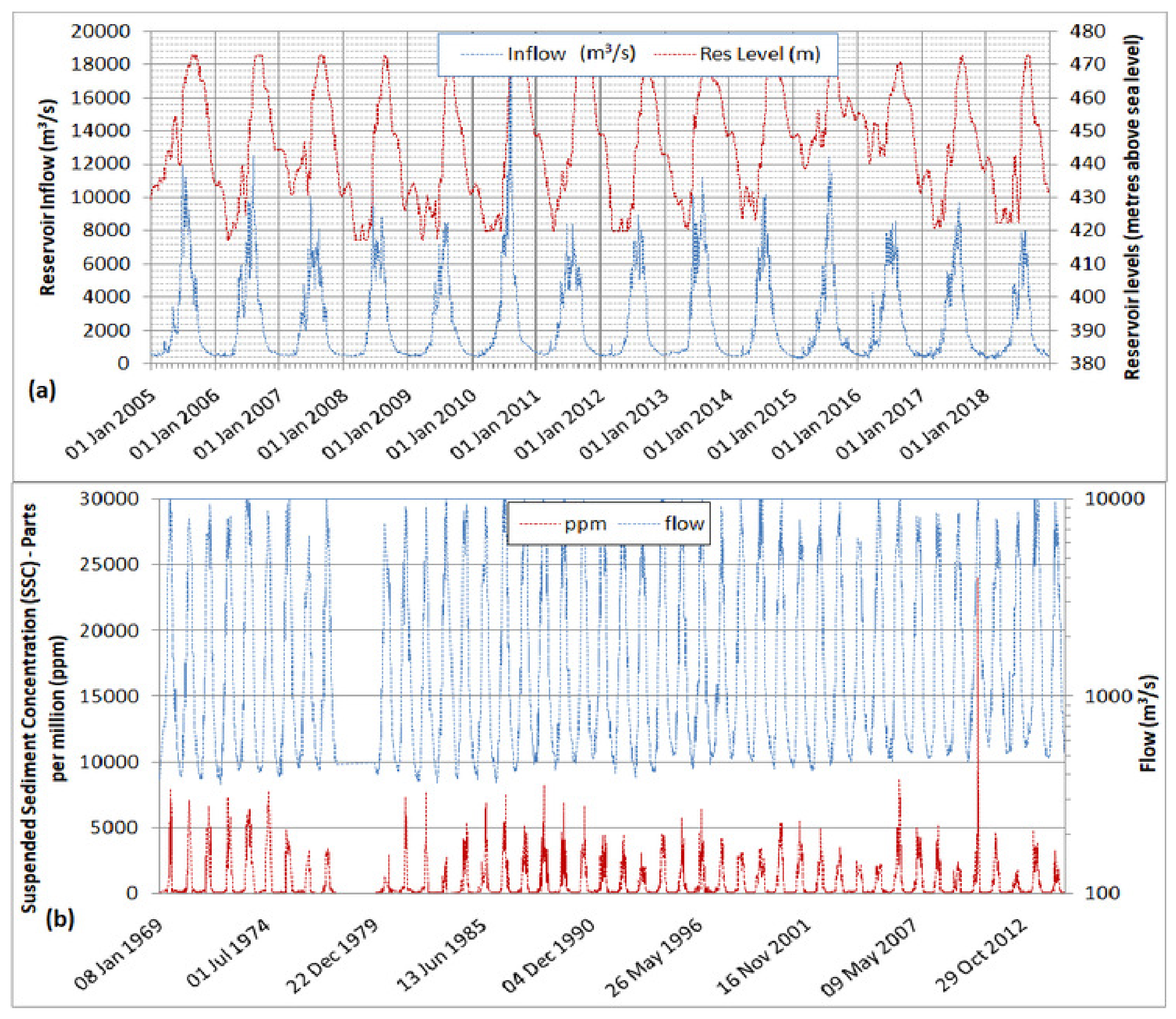
In the numerical model, daily reservoir water levels (RWLs) of the Tarbela Reservoir were applied for the downstream boundary condition. At the upstream boundary, we specified daily inflows with corresponding sediment load. Modeled results were compared to observations and evaluated based on the statistical performance parameters like the coefficient of determination (R2), the observations standard deviations ratio (RSR), and the Nash–Sutcliffe Efficiency (NSE).
Actual daily inflows of 14 years (2005–2018) were given as the upper flow boundary condition for running the model with the SRC-based sediment loads and were repeated thereafter up to 2030. For running the model with the WA-ANN-based sediment loads, actual daily inflows from 2005–2018 and thereafter futuristic flows from 2019–2030 as projected by [35] under plausible near-future climatic conditions were applied as upper boundary conditions. Actual daily RWLs of the Tarbela Reservoir were given as the downstream boundary condition up to 2018 and repeated thereafter for both SRC and WA-ANN runs of the model.
To check the performance of the SRC method (Equations (1) and (2)), sediment loads were generated and matched against observed sediment loads. The sediment equations output sediment load in t/day by the input of flow in m3/s. The generated/estimated sediment load was matched against observed sediment load entering the reservoir for that particular day. The observed sediment load was calculated by converting observed sedimentation concentration in mg/L for that day into t/day by carrying out a dimensional analysis. The calculated values of NSE, R2, and RSR were 0.635, 0.655, and 0.076, respectively, amply proving that the SRC technique, although in vogue, predicted output with an unacceptable level of certainty.
Applying the concept of data preprocessing on Besham Qila gauge station’s data developed by [41], where he found the best relationship by selecting 70% of the input data for training, 15% for testing, and 15% for validation, we also obtained better results for the time period 1969–2014. The 70%, 15%, and 15% data from the entire available series was randomly selected for training, testing, and validation processes, respectively. It is also worthwhile to mention here that data pre-processing plays an important role where a short duration data series is available; however, our data series of more than 40 years also provided us the best results on even specifying 60% of data for training, 20% for testing, and the remaining 20% for validation. The coefficient of determination (R2) for the training and testing datasets was 0.780 and 0.743, respectively. The Nash–Sutcliffe efficiency (NSE) was also 0.780 and 0.742 for training and testing, respectively. As our ANN trained best using single decomposition on Q(t), the inputs were only detailed and approximated coefficients of discharge without lag-time. The best trained WA-ANN used “tainsig” transfer functions in both the hidden and output layers. The number of hidden neurons in the single hidden layer of ANN was only five compared to seven for the same gauge station in [41]. As the Levenberg–Marquardt algorithm has fast convergence and also performed well for the Indus River [4], it also performed best in our training. The simulations stopped when the difference between the last and second to last simulation was less than 1/1000 or it reached maximum epochs of 1000 iterations. The work in [41] used the data series from 1969–2008 and reconstructed missing data for the Tarbela Reservoir with R2 = 0.773 and 0.794 for testing and training, respectively. The statistical performance of our WA-ANN with a larger data series up to 2014 was slightly better for training data; however, it was slightly lower for testing data, which may be due to the inclusion of the exceptionally high flood of 2010. Similarly, increasing the decomposition levels slightly affected the model performance, which, interestingly, was significantly improved in [41]. In addition, the WA-ANN-generated sediment series showed an annual 160 Mt of suspended sediment load (excluding 10% bed load) entering the Tarbela Reservoir, which was similar to the estimate of [41].

3.1. Model Calibration

The model was calibrated for a period of nine years (2005–2013). The gradational analysis showed that on average, the Indus River transported silt (56.68%) as compared to sand (33.94%) and clay (9.78%).
Further, an extensive analysis of available particle size data of Besham Qila gauging station for 1983, 1989, 1991, 1994, and from 2002–2012 was conducted to calculate its variations with flow. Firstly, as mentioned in the previous paragraph, the average percentages for sand-, silt-, and clay-sized particles were calculated for all flow conditions. Then, the data were segregated into different sets corresponding to the indicated flow ranges in Table 4, and average percentages for sand-, silt-, and clay-sized particles were calculated for those particular flow ranges/bands. The analysis showed conclusively that the percentages of gradations across the sediment classes changed significantly with changing flow bands and were liable to affect sediment transport behavior as the flows increase/decrease. This analysis was important to study and model the morphodynamics across changing low and high flow bands accurately. The results are shown in Table 4 and entered in the sediment module of HEC-RAS as an adjunct to SRC and WA-ANN load series.
First, only hydrodynamic calibration was carried out up to 2013 by changing the value of Manning’s roughness (n) throughout the length of the reservoir and comparing the calculated water levels with the observed water levels at different locations along the 66 available cross-sections. Initially, a uniform hydraulic roughness n = 0.04 from the literature [42,43] was adopted and subsequently adjusted in a plausible range of 0.035–0.04, throughout the 73 R/Lines of the reservoir and by comparing with available observed water levels, achieving an NSE and R2 of 0.916 and 0.940, respectively. Next, hydro-morphodynamic calibration was attempted by varying both bed roughness and sediment parameters in the model.
Applying SRC sediment load at the inlet, it was noticed that the Ackers–White transport formula with the sorting method of Exner (7) was producing somewhat higher values of NSE and R2. Exner (5) and Exner (7) are common bed sorting methods (sometimes called the mixing or armoring methods), which keep track of the bed gradation used by HEC-RAS to compute grain size-specific capacities and also to simulate armoring processes. Exner (5) uses a three-layer bed model that forms an independent coarse armor layer, which limits the erosion of deeper layers, whereas Exner (7) is an alternate version of Exner (5) designed for sand bed rivers as it forms armor layers more slowly and computes more erosion.
Hence, by keeping the combination of Ackers–White + Exner (7) constant, different fall velocities were tested to better the results. Amongst provisions to input commonly-used fall velocity methods like van Rijn, Ruby, and Tofaletti, HEC-RAS has an option to input the Report 12 fall velocity method, which finds solution iteratively by using the same curves as van Rijn, but using the computed fall velocity to compute the new Reynolds number until the assumed velocity matches with the computed velocity within tolerable limits. Consequently, a third tier calibration effort was attempted by varying scaling factors for transport and mobility functions of the transport formula as allowed by the HEC-RAS model for calibration fine-tuning, the result of which emerged with NSE and R2 of 0.943 and 0.959, respectively. The default value of scaling factors was one, which was manipulated to achieve the maximum hydrodynamic calibration of NSE and R2 of 0.996. It is worth mentioning here that for the sediment simulation and management study in Tarbela Reservoir in 1998 [44], the Ackers–White transport formula [45] was selected. The work in [43] also suggested the adoption of the Ackers–White formula, for the total load transport capacity of sand-sized fractions. However, other formulas were also tested in the calibration process as detailed in Table 5. A comparison with observed bed levels of 2013 was made and presented in Figure 7.
Further, another extensive calibration exercise was carried out applying WA-ANN-based boundary conditions. Again, the Ackers–White transport formula with the sorting method of Exner (5) showed better results. Next, the above combination (Ackers–White + Exner-5) was evaluated by changing the fall velocity equations. Similar to the SRC case, the Tofaletti technique showed the best results hitherto, prior to application of scaling factors. Consequently, the best combination of input parameters (Ackers–White + Exner-7 + Tofaletti) was subjected to rigorous scaling of transport formula parameters. Hence, the highest NSE of 0.979 was achieved during calibration, and the results of the exercise tabulated in Table 6 in increasing order of NSE values. A comparison with observed bed levels of 2013 was made and presented in Figure 8.

3.2. Model Validation

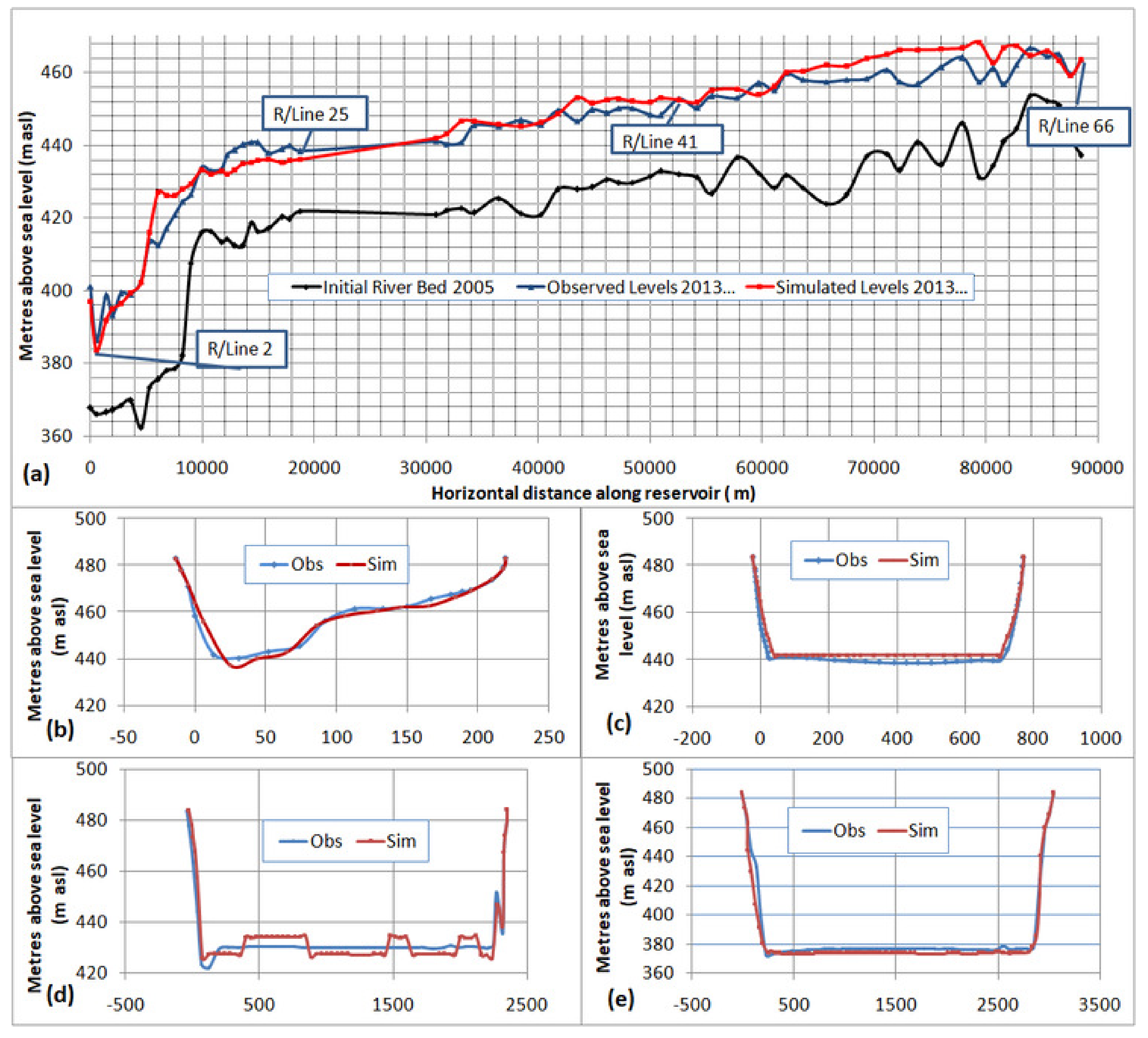
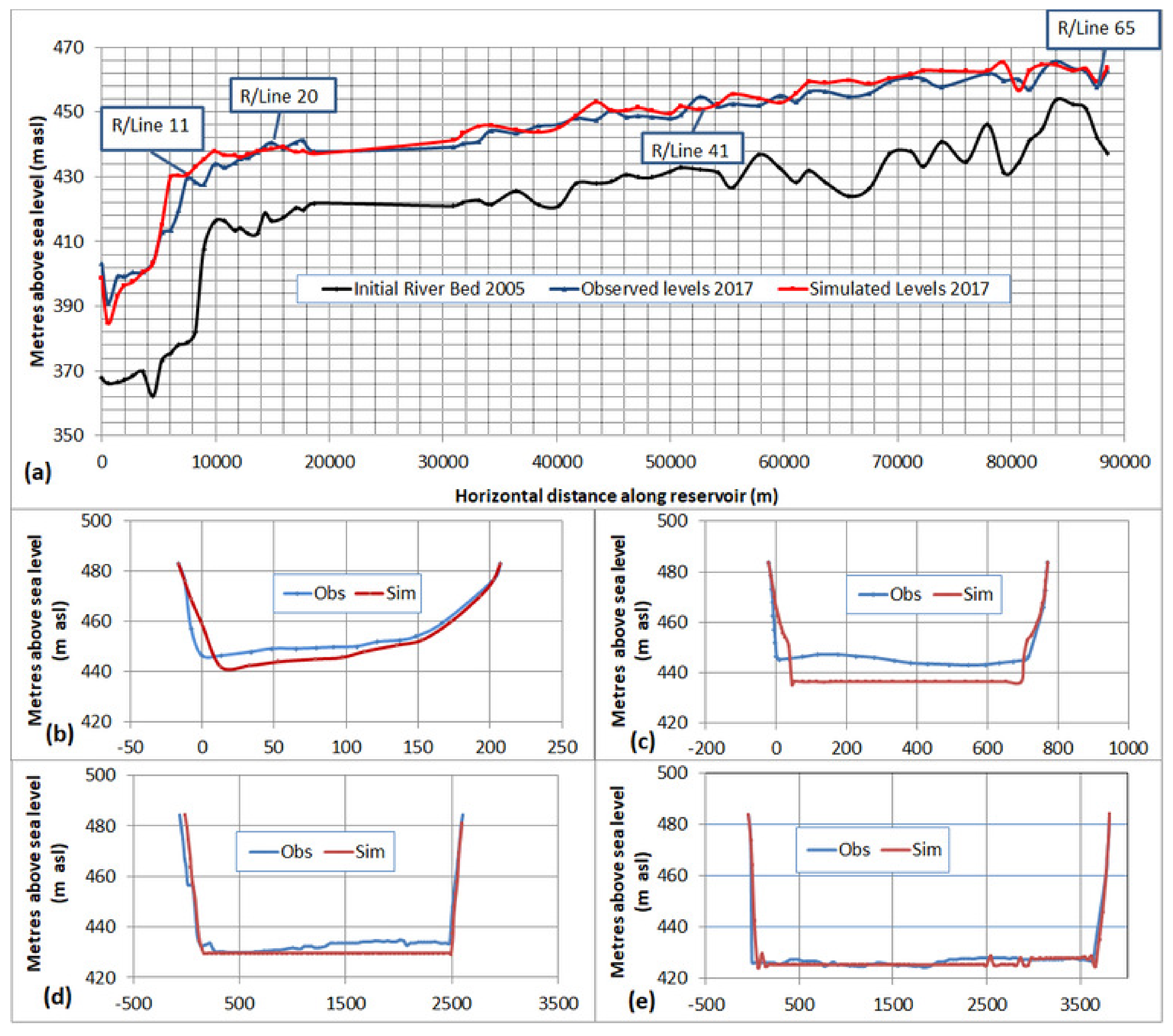
To validate the HEC-RAS model with the SRC technique, it was run for another four years up to 2017. The output was compared with observed sediment deposits of 2017 and is presented in Figure 9.
The R2 and NSE in the validation process were 0.950 and 0.893, respectively. The observed standard deviation was at 0.041. In a recent study [46], the HEC-RAS model was validated for the Tarbela Reservoir by simulating it only for one year, and an approximately 20-m difference between the observed and simulated river beds for the sediment delta in the year 2000 was found. However, in the present study, the difference of four years of simulation was only 4–5 m in the whole longitudinal profile (Figure 9). A better modeling performance might be due to more accurate sediment load boundary conditions generated using a long-term data series, i.e., 1969–2014, whereas [46] used only a 28-year data series, i.e., 1979–2006.
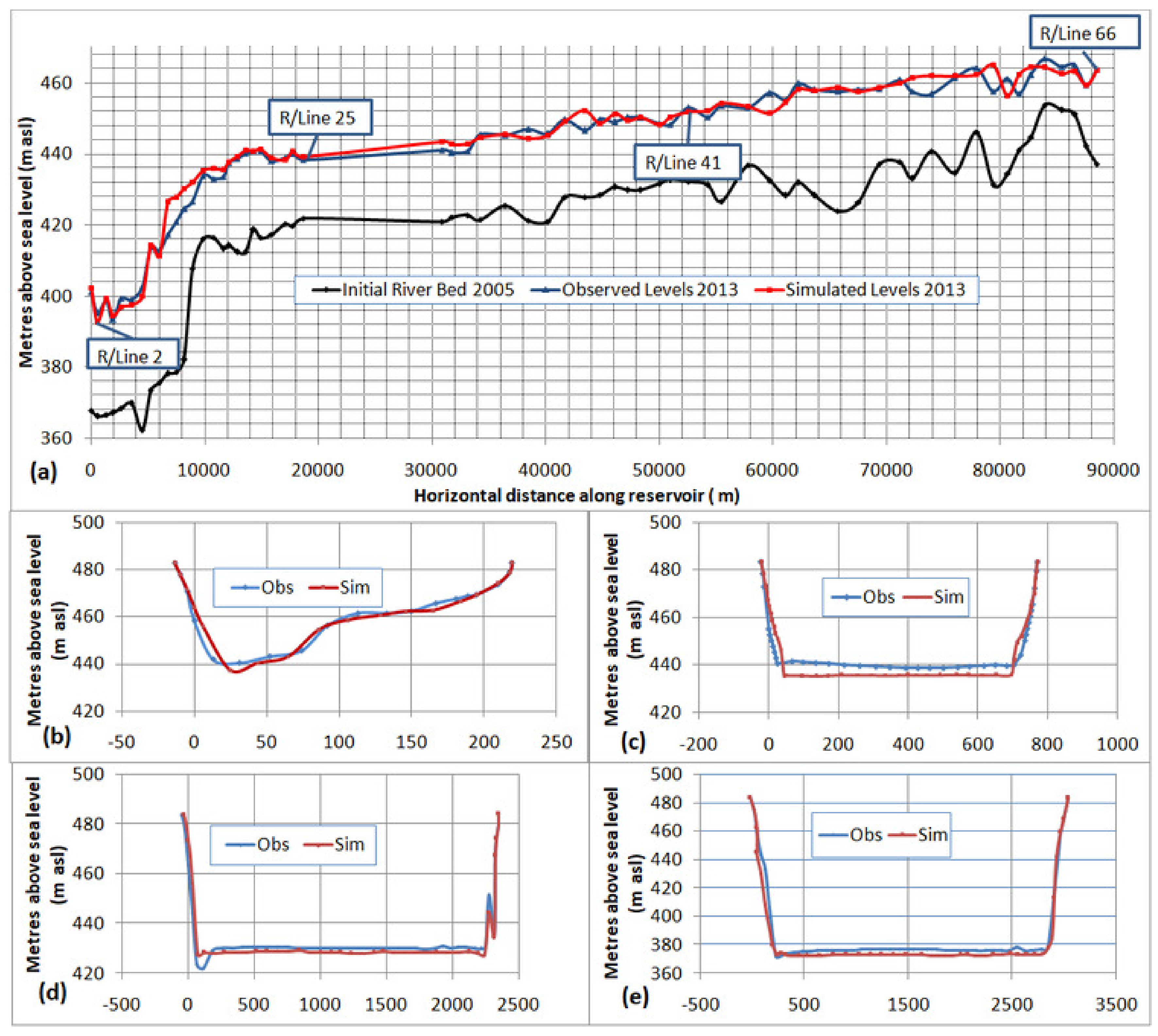
To validate the HEC-RAS model with the above calibrated WA-ANN sediment series, it was run for another four years up to 2017, similar to the SRC model. The output was compared with observed sediment deposits of 2017 and presented in Figure 10. The R2 and NSE in the validation process were 0.968 and 0.959, respectively. The observed standard deviation was at 0.025.

3.3. HEC-RAS Model Performance with the SRC and WA-ANN Techniques

To sum up the above-elaborated calibration and validation exercises using SRC and WA-ANN-based boundary conditions, their statistical performance was compared and tabulated in Table 7. The statistical results (Table 7) clearly indicated a preferable performance of the model using WA-ANN-based sediment load boundary conditions. As SRC reconstructed the missing sediment load data with R2 and NSE at 0.635 and 0.655, respectively, the model calibration took a long time to adjust transport parameters for attaining stability. However, due to better recondition accuracy using WA-ANN (R2 = 0.771 and NSE = 0.771), the HEC-RAS model simulated the bed-levels changes with great stability. As the SRC overestimated sediment load, therefore to flush extra sediments, we needed to adjust the transport parameters that might not represent the correct physics of the transport processes in the reservoir. Therefore, more accurate boundary conditions played a vital role in precise modeling of the transport processes by keeping transport parameters within the physical limits.

3.4. Models’ Application for Sediment Delta Prediction

More than 200 million people of Pakistan directly or indirectly depend on the irrigation supply and power generation from the Tarbela Dam. Therefore, it is very important to assess the future delta movement and sedimentation scenarios in the reservoir. It is pertinent to mention here that SRC-generated sediment load boundary conditions are being used for all types of sedimentation modeling in the upper Indus River projects [21,42]. Therefore, to check and ascertain the long-term application of the SRC and WA-ANN techniques, the HEC-RAS model was run up to the year 2030 using future discharges calculated by [35] employing the University of British Columbia (UBC) watershed model. UBC is a less data-extensive semi-distributed watershed model developed by the University of British Columbia. As discharge alone with one level of decomposition represents more accurately the transport processes at Besham Qila, calculated future discharges by [
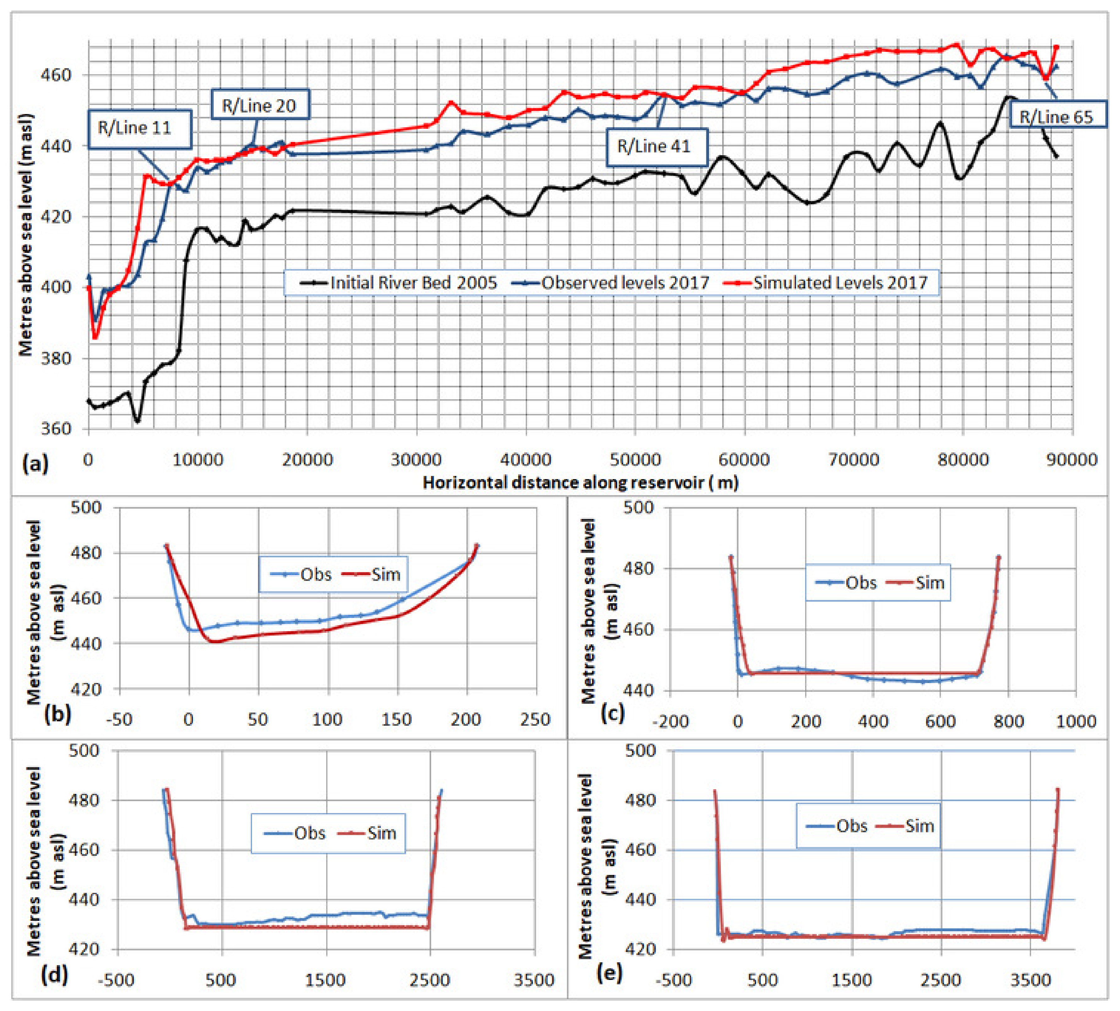
35] were used in the trained WA-ANN model for obtaining future sediment loads. Reservoir water levels from 2005–2018 were repeated for 2019–2030. The simulated/forecasted levels of the Tarbela Reservoir for 2022 and 2030 along with observed levels of 2013 and 2017 showed a huge volume lost due to sedimentation (see Figure 11). As SRC showed overestimation (190 Mt of suspended sediment load (SSL) compared to 160 Mt SSL using WA-ANN) for the Indus River (Table 1), therefore, using SRC as the boundary condition in the modeling process also overestimated the bed level variations in the major ponding area of the reservoir near the dam. As SRC has been used for sedimentation modeling of all studies of the Upper Indus River, and it has been predicting similar results. For example, the 4320-MW Dasu Hydropower Project, which is under construction upstream of Tarbela Dam, will be silted up just 20–25 years after its commissioning without conducting yearly flushing operations [21,41]. The predicted short life of the Dasu project could very likely be a result of the overestimation of sediment load using SRCs. Initially, the work in [13] in 1970 also estimated 400 Mt of sediment load using SRC for the Tarbela Reservoir, which showed a shorter life of the reservoir. However, later studies estimated 50% lower sediment load for the Indus River at Tarbela Dam (see Table 1). Due to less sediments entering the reservoir, it is still operational and not silted-up. It might be possible that in 1970, very limited sediment concentration data were available, which might have consisted of high-flow hydrological years. However, the availability of long data series of sediment sampling cannot help SRC to model the hysteresis phenomenon and hydrological variations related to shifting in high flows from summer to post- and pre-summer months at the Upper Indus Basin [41]. Therefore, the WA-ANN-generated sediment load boundary condition, using future projected discharges, can more precisely represent the sedimentation modeling processes.

4. Conclusions

In the present study, the performance of HEC-RAS 1D model for modeling morphodynamic processes in the Tarbela Reservoir was tested using sediment rating curves and WA-ANN-based sediment load boundary conditions. A data series from 2005–2013 was used in the calibration, while a data series from 2014–2017 was used in the validation process. Based on the study results, the following conclusions can be drawn:
  • Compared to sediment rating curves, the WA-ANN model better represented the hysteresis phenomenon for the Indus River and could reconstruct the missing sediment load more accurately.
  • More accurate sediment load boundary conditions enabled the numerical model to calculate the bed level changes more precisely and also to provide stability in the calculation process. By comparing Figure 7d and Figure 8d, it is evident that the simulated bed with WA-ANN showed stability against the SRC-simulated bed.
  • A de-synchronization between glacier melt and rainfall in the upper Indus catchment will cause a decrease in sediment to the Tarbela Reservoir and will decrease the sedimentation rate.
On the basis of the above conclusions, the following recommendations are being put forward:
  • Sediment rating curves should not be utilized to design the reservoir sediment management rules for the existing, under construction, or planned projects in the upper Indus Basin, as they cannot adjust the hysteresis phenomenon and contribute variations in the sediment load boundary conditions.
  • As we have repeated 2005–2018 reservoir operational rules for 2019–2030 in the modeling process, the future reservoir operational rules should be optimized to keep sediment delta stable.

Author Contributions

Z.R.T. defined the problem, outlined the research plan, carried out the research, and interpreted and drafted the outcome. S.R.A. calculated and analyzed flow and sediment concentration data, prepared SRCs, and made significant contributions to improve the draft. S.u.H. contributed the hydrological model for future flows of the Indus River. S.A.-U.-R. and M.D.B. developed WA-ANN models for setting sediment load boundary conditions and helped in the preparation of this paper with proof reading and corrections. R.M.A.W. collected/collated all the relevant data from different sources. Z.M.K. and I.A. supervised and directed the research study and reviewed the end result critically.

Funding

This research received no external funding.

Acknowledgments

The study data were provided by the Tarbela Dam Organisation of WAPDA upon specific request of College of Earth and Environmental Sciences (CEES). We appreciate their help and cooperation. Shabeh ul Hasson also acknowledges the support and funding from the Deutsche Forschungsgemeinschaft (DFG, German Research Foundation) through the Cluster of Excellence ‘CliSAP’ (EXC177), and under Germany‘s Excellence Strategy –EXC 2037 ‘CLICCS - Climate, Climatic Change, and Society’ –Project Number: 390683824, contribution to the Center for Earth System Research and Sustainability (CEN) of Universität Hamburg. The corresponding author is also grateful to Rohit Kumar, DNZE Munich, for his help.

Conflicts of Interest

The authors declare no conflicts of interest.

References

  1. Hassan, M.; Shamim, M.A.; Sikandar, A.; Mehmood, I.; Ahmed, I.; Ashiq, S.Z.; Khitab, A. Development of sediment load estimation models by using artificial neural networking techniques. Environ. Monit. Assess. 2015, 187, 1–13. [Google Scholar] [CrossRef] [PubMed]
  2. Colby, B. Relationship of Sediment Discharge to Streamflow; United States Geological Survey: Reston, VA, USA, 1956. [Google Scholar]
  3. Glysson, G. Sediment-Transport Curves; United States Geological Survey: Reston, VA, USA, 1987. [Google Scholar]
  4. Ateeq-Ur-Rehman, S.; Bui, M.D.; Rutschmann, P. Variability and trend detection in the sediment load of the Upper Indus River. Water 2018, 10, 1–16. [Google Scholar] [CrossRef]
  5. Ateeq-Ur-Rehman, S.; Bui, M.D.; Hasson, S.U.; Rutschmann, P. An Innovative Approach to Minimizing Uncertainty in Sediment Load Boundary Conditions for Modeling Sedimentation in Reservoirs. Water 2018, 10, 1411. [Google Scholar] [CrossRef]
  6. Survey and Hydrology. Annual Report on Tarbela Reservoir Sedimentation—2011; Water and Power Development Authority (WAPDA): Lahar, Pakistan, 2012. [Google Scholar]
  7. Asianics Agro-Dev. International (Pvt) Ltd. Tarbela Dam and Related Aspects of the Indus River Basin, Pakistan, A WCD Case Study Prepared as an Input to the World Commission on Dams; Asianics Agro-Dev. International (Pvt) Ltd.: Islamabad, Pakistan, 2000. [Google Scholar]
  8. Office of Superintending Engineer, Survey & Hydrology Residency. Tarbela Reservoir Capacity Table—2019; Wapda: Lahore, Pakistan, 2019. [Google Scholar]
  9. Consultants, G.G.H. Technical Report No. 3, Sedimentology of Ghazi-Garriala Hydropower Project, Feasibility Report; Technical Report; Water and Power Development Authority: Lahore, Pakistan, 1991. [Google Scholar]
  10. Consultants, D.B. Reservoir Sedimentation Studies, Appendix C to Reservoir Operation and Sediment Transport; Technical Report; Water and Power Development Authority: Lahar, Pakistan, 2007. [Google Scholar]
  11. Ateeq-Ur-Rehman, S.; Bui, M.D.; Rutschmann, P. Detection and estimation of sediment transport trends in the upper Indus River during the last 50 years. Hydropower: A Vital Source of Sustainable Energy for Pakistan; Sarwar, K., Ahmad, I., Eds.; Center of Excellence in Water Resources Engineering: Lahore, Pakistan, 2017; pp. 1–6. [Google Scholar]
  12. Holeman, J.N. The sediment yield of major rivers of the world. Water Resour. Res. 1968, 4, 737–747. [Google Scholar] [CrossRef]
  13. Peshawar University. The Sediment Load and Measurements for Their Control in Rivers of West Pakistan; Department of Water Resources: Peshawar, Pakistan, 1970. [Google Scholar]
  14. Meybeck, M. Total mineral dissolved transport by world major rivers/Transport en sels dissous des plus grands fleuves mondiaux. Hydrol. Sci. J. 1976, 21, 265–284. [Google Scholar] [CrossRef]
  15. Lowe, J.; Fox, I. Sedimentation in Tarbela reservoir. In Commission Internationale des Grandes Barrages (International Commission on Large Dams-ICOLD, Paris, France); Quatorzieme Congres des Grands Barrages: Rio de Janeiro, Brazil, 1982. [Google Scholar]
  16. Roca, M.; Tarbela Dam in Pakistan. Case study of reservoir sedimentation. In Proceedings of River Flow; Munoz, R.E.M., Ed.; CRC Press: London, UK, 2012. [Google Scholar]
  17. Milliman, J.; Quraishee, G.; Beg, M. Sediment discharge from the Indus River to the ocean: Past, present and future. In Marine Geology and Oceanography of Arabian Sea and Coastal Pakistan; Haq, B.U., Milliman, J.D., Eds.; van Nostrand Reinhold/Scientific and Academic Editions: New York, NY, USA, 1984; pp. 65–70. [Google Scholar]
  18. Summerfield, M.A.; Hulton, N.J. Natural controls of fluvial denudation rates in major world drainage basins. J. Geophys. Res.-Solid Earth 1994, 99, 13871–13883. [Google Scholar] [CrossRef]
  19. Collins, D. Hydrology of Glacierised Basins in the Karakoram: Report on Snow and Ice Hydrology Project in Pakistan with Overseas Development Administration, UK [ODA] and Water and Power Development Authority, Pakistan [WAPDA]; University of Manchester: Manchester, UK, 1994. [Google Scholar]
  20. Ali, K.F. Construction of Sediment Budgets in Large Scale Drainage Basins: The Case of the Upper Indus River. Ph.D. Thesis, Department of Geography and Planning, University of Saskatchewan, Saskatoon, SK, Canada, 2009. [Google Scholar]
  21. Dasu Hydropower Consultants. Detailed Engineering Design Report, Part A; Engineering Design; Water and Power Development Authority: Lahar, Pakistan, 2013. [Google Scholar]
  22. Graf, W.H. Hydraulics of Sediment Transport; Water Resources Publication: Littleton, CO, USA, 1984. [Google Scholar]
  23. McBean, E.A.; Al-Nassri, S. Uncertainty in suspended sediment transport curves. J. Hydraul. Eng. 1988, 114, 63–74. [Google Scholar] [CrossRef]
  24. Morris, G.L.; Fan, J. Reservoir Sedimentation Handbook: Design and Management of Dams, Reservoirs, and Watersheds for Sustainable Use; McGraw Hill Professional: New York, NY, USA, 1998. [Google Scholar]
  25. Bogen, J. The hysteresis effect of sediment transport systems. Nor. Geogr. Tidsskr.-Nor. J. Geogr. 1980, 34, 45–54. [Google Scholar] [CrossRef]
  26. Hewitt, K. Gifts and perils of landslides: Catastrophic rockslides and related landscape developments are an integral part of human settlement along upper Indus streams. Am. Sci. 2010, 98, 410–419. [Google Scholar]
  27. Partal, T.; Kucuk, M. Long-term trend analysis using discrete wavelet components of annual precipitations measurements in Marmara region (Turkey). Phys. Chem. Earth 2006, 31, 1189–1200. [Google Scholar] [CrossRef]
  28. Adamowski, K.; Prokoph, A.; Adamowski, J. Development of a new method of wavelet aided trend detection and estimation. Hydrol. Process. 2009, 23, 2686–2696. [Google Scholar] [CrossRef]
  29. Railean, I.; Moga, S.; Borda, M.; Stolojescu, C.L. A wavelet based prediction method for time series. In Stochastic Modeling Techniques and Data Analysis (SMTDA2010); Janssen, J., Ed.; ASMDA International: Chania, Greece, 2010. [Google Scholar]
  30. Tan, C.; Huang, B.S.; Liu, K.S.; Chen, H.; Liu, F.; Qiu, J.; Yang, J.X. Using the wavelet transform to detect temporal variations in hydrological processes in the Pearl River, China. Quat. Int. 2017, 440, 52–63. [Google Scholar] [CrossRef]
  31. Tarar, Z.R.; Ahmad, S.R.; Ahmad, I.; Majid, Z. Detection of Sediment Trends Using Wavelet Transforms in the Upper Indus River. Water 2018, 10, 918. [Google Scholar] [CrossRef]
  32. Brunner, G.W. HEC-RAS River Analysis System, Hydraulic Reference Manual; US Army Corps of Engineers: Washington, DC, USA, 2016. [Google Scholar]
  33. Hewitt, K. The Karakoram Anomaly? Glacier Expansion and the ‘Elevation Effect’, Karakoram Himalaya. Mt. Res. Dev. 2005, 25, 332–340. [Google Scholar] [CrossRef]
  34. Lutz, A.F.; Immerzeel, W.W.; Kraaijenbrink, P.D.A.; Shrestha, A.B.; Bierkens, M.F.P. Climate Change Impacts on the Upper Indus Hydrology: Sources, Shifts and Extremes. PLoS ONE 2016, 11, e0165630. [Google Scholar] [CrossRef] [PubMed]
  35. Hasson, S.U. Future Water Availability from Hindukush-Karakoram-Himalaya upper Indus Basin under Conflicting Climate Change Scenarios. Climate 2016, 4, 40. [Google Scholar] [CrossRef]
  36. Wijngaard, R.R.; Lutz, A.F.; Nepal, S.; Khanal, S.; Pradhananga, S.; Shrestha, A.B.; Immerzeel, W.W. Future changes in hydro-climatic extremes in the Upper Indus, Ganges, and Brahmaputra River basins. PLoS ONE 2017, 12, e0190224. [Google Scholar] [CrossRef]
  37. Bonekamp, P.N.J.; de Kok, R.J.; Collier, E.; Immerzeel, W.W. Contrasting Meteorological Drivers of the Glacier Mass Balance Between the Karakoram and Central Himalaya. Front. Earth Sci. 2019, 7, 107. [Google Scholar] [CrossRef]
  38. Organization, W.M. WMO Statement on the State of the Global Climate in 2018; World Meteorological Organization (WMO): Geneva, Switzerland, 2019. [Google Scholar]
  39. Nash, J.; Sutcliffe, J. River flow forecasting through conceptual models, part I: A discussion of principles. J. Hydrol. 1970, 10, 282–290. [Google Scholar] [CrossRef]
  40. Dixit, A.; Majumdar, S. Comparative analysis of Coiflet and Daubechies wavelets using global threshold for image denoising. Int. J. Adv. Eng. Technol. 2013, 6, 2247–2252. [Google Scholar]
  41. Ateeq-Ur-Rehman, S. Numerical Modeling of Sediment Transport in Dasu-Tarbela Reservoir Using Neural Networks and TELEMAC Model System. Ph.D. Thesis, Chair of Hydraulic and Water Resources Engineering, Technical University of Munich (TUM), Munich, Germany, 2019. [Google Scholar]
  42. Dasu Hydropower Project. Dasu Hydropower Project, Feasibility Report; Water and Power Development Authority: Lahore, Pakistan, 2009. [Google Scholar]
  43. HR Wallingford. Sedimentation Study, Dasu Hydropower Project, Pakistan; Report EX 6801 R1; Dasu Hydropower Consultants: Pakhtunkhwa, Pakistan, 2012. [Google Scholar]
  44. Wallingford, T.C.I.H. Tarbela Dam Sediment Management Study; Wapda: Lahore, Pakistan, 1998; Volume 2. [Google Scholar]
  45. Ackers, P.; White, W.R. Sediment Transport: New Approach and Analysis. ASCE Hydr. Div. J. 1973, 99, 2041–2060. [Google Scholar]
  46. Rehman, H.U.; Rehman, M.A.; Naeem, U.A.; Hashmi, H.N.; Shakir, A.S. Possible options to slow down the advancement rate of Tarbela delta. Environ. Monit. Assess. 2018, 190, 39. [Google Scholar] [CrossRef] [PubMed]
Figure 1. Demarcated Upper Indus Basin at Tarbela Dam.
Water 11 01716 g001
Figure 2. Data used in the study: (a) daily Tarbela Reservoir inflow and levels; (b) occasionally-collected suspended sediment concentration samples with observed flow.
Water 11 01716 g002
Figure 3. Range lines (R/Lines) of Tarbela Reservoir used from [5].
Water 11 01716 g003
Figure 4. Sediment rating curve.
Water 11 01716 g004
Figure 5. Monthly sediment load at Besham Qila with sediment rating curves (SRC).
Water 11 01716 g005
Figure 6. Daubechies wavelet families.
Water 11 01716 g006
Figure 7. Comparison of observed and SRC simulated bed levels during calibration for 2013: (a) along the Tarbela Reservoir; (b) R/Line 66; (c) R/Line 41; (d) R/Line 25; (e) R/Line 2.
Water 11 01716 g007
Figure 8. Comparison of observed and WA-ANN-simulated bed levels during calibration for 2013: (a) along the Tarbela Reservoir; (b) R/Line 66; (c) R/Line 41; (d) R/Line 25; (e) R/Line 2.
Water 11 01716 g008
Figure 9. Comparison of observed and SRC simulated bed levels during validation for 2017: (a) along the Tarbela Reservoir; (b) R/Line 65; (c) R/Line 41; (d) R/Line 20; (e) R/Line 11.
Water 11 01716 g009
Figure 10. Comparison of observed and WA-ANN-simulated bed levels during validation for 2017: (a) along Tarbela Reservoir; (b) R/Line 65; (c) R/Line 41; (d) R/Line 20; (e) R/Line 11.
Water 11 01716 g010
Figure 11. Comparison of simulated bed levels for 2022 and 2030 with the SRC and WA-ANN techniques, along with observed levels of 2013 and 2017. The longitudinal profile is only showing the sediment delta region of Tarbela Dam.
Water 11 01716 g011
Table 1. Published estimates of sediment load (SL) of the Upper Indus River.
Sediment Load (Mt year−1)Estimate by
480[12]
400[13]
475[14]
200[15] as per the report by [16]
675[17]
300[18]
200[19]
197[20]
200[21]
Table 2. Statistical performance parameters used to evaluate the modeling performance.
ParametersDescriptionRanges
Coefficient of determination R 2 = i = 1 P ( X i o b s X ¯ o b s ) ( X i s i m X ¯ s i m ) i = 1 P ( X i o b s X ¯ o b s ) 2 i = 1 P ( X i s i m X ¯ s i m ) 2 2 0–1
Observations standard deviation ratio (RSR) R S R = R M S E S T D E V o b s = 1 P i = 1 P ( X i o b s X i s i m ) 2 i = 1 P ( X i o b s X ¯ o b s ) 2 0–1
Nash–Sutcliffe efficiency (NSE) N S E = 1 i = 1 P ( X i o b s X i s i m ) 2 i = 1 P ( X i o b s X ¯ o b s ) 2 –1
X i o b s , X i s i m represent the i th observed and simulated value of parameters. X ¯ represents the mean.
Table 3. Average monthly load in Mt at Besham Qila with SRC.
JanFebMarAprMayJunJulAugSepOctNovDecAnnual
0.0370.0260.0680.3745.17138.61387.88466.2859.8000.6060.1540.077212.068
Table 4. Gradation percentages vis-à-vis increasing flow bands.
Flow Ranges (m3/s)Clay (%)Silt (%)Sand (%)
up to 14165.551.343.1
up to 283210.349.839.8
up to 42489.454.436.2
up to 56637.150.042.9
up to 70798.656.834.6
up to 84958.857.234.0
up to 991110.966.023.1
up to 11,327 and above17.568.014.5
Table 5. Statistical performance of HEC-RAS with SRC sediment series by the input of different transport formulae and varying parameters.
Sed Transport FormulaeSorting MethodFall VelocityScaling Factors AppliedNSER2
YangExner (5)van RijnNo0.8170.943
Laursen-CopelandExner (5)van RijnNo0.8590.948
Engelund-HansenExner (5)van RijnNo0.8670.950
Ackers–WhiteExner (5)van RijnNo0.8690.952
Ackers–WhiteExner (7)van RijnNo0.8960.956
Ackers–WhiteExner (7)RubyNo0.8970.955
Ackers–WhiteExner (7)Report 12No0.8980.956
Ackers–WhiteExner (7)TofalettiNo0.9080.964
Ackers–WhiteExner (7)TofalettiYes0.9430.959
Table 6. Statistical performance of HEC-RAS with WA-ANN sediment series by the input of different transport formulae and varying parameters.
Sed Transport FormulaeSorting MethodFall VelocityScaling Factors AppliedNSER2
Ackers–WhiteExner (7)van RijnNo0.8290.975
Laursen-CopelandExner (7)van RijnNo0.8300.975
YangExner (7)van RijnNo0.8300.974
Engelund-HansenExner (7)van RijnNo0.8310.976
YangExner (5)van RijnNo0.8320.966
Engelund-HansenExner (5)van RijnNo0.8550.969
Laursen-CopelandExner (5)van RijnNo0.8630.970
Ackers–WhiteExner (5)Report 12No0.8690.971
Ackers–WhiteExner (5)RubyNo0.8690.970
Ackers–WhiteExner (5)van RijnNo0.8700.970
Ackers–WhiteExner (5)TofalettiNo0.8760.972
Ackers–WhiteExner (5)TofalettiYes0.9790.980
Table 7. Statistical performance of HEC-RAS model with the SRC and WA-ANN techniques during the calibration and validation periods.
ProcessDurationR2RSRNSE
SRCWA-ANNSRCWA-ANNSRCWA-ANN
Calibration2005–20130.9590.9800.0300.0180.9430.979
Validation2014–20170.9500.9680.0410.0250.8930.959

