Fish Response to Turbulence Generated Using Multiple Randomly Actuated Synthetic Jet Arrays
by
 , ,
, ,
Samuel F. Harding
1,*, 
Robert P. Mueller
1,
Marshall C. Richmond
1,
Pedro Romero-Gomez
2 and
Alison H. Colotelo
1 1
Pacific Northwest National Laboratory, Richland, WA 99352, USA
2
ANDRITZ HYDRO GmbH, 4031 Linz, Austria
*
Author to whom correspondence should be addressed.
Water 2019, 11(8), 1715; https://doi.org/10.3390/w11081715
Submission received: 16 May 2019
/
Revised: 27 June 2019
/
Accepted: 18 July 2019
/
Published: 17 August 2019
(This article belongs to the Section Hydraulics and Hydrodynamics)
Abstract
:Hydroelectric power stations generate turbulent flow conditions, which represent a potentially significant hydraulic stressor to fish passing through the turbine system. A test facility has been developed using two randomly actuated synthetic jet arrays (RASJAs) of 25 independent submersible pumps to generate a turbulent flow field for biological dose-response testing. The novel elements of this approach include the ability to control the exposure duration within a test volume due to low mean flow velocity as well as the capacity to scale the turbulence levels as a function of pump capacity. Juvenile Chinook salmon (Oncorhynchus tshawytscha) were subjected to the turbulent flow regime with average turbulence kinetic energy per unit mass of for periods of 2 min and 10 min. No significant loss of equilibrium or disorientation was observed after exposure for either duration at the level of turbulence achieved in this prototype. Further scaling of this approach is required to generate a complete dose-response relationship.
1. Introduction
1.1. Background
The successful passage of fish through power stations is an important regulatory and ecological consideration of hydro sites. In particular, the downstream navigation of a hydro electric power station poses a range of risks to both anadromous and resident fish populations including contact with turbine components, changes in velocity, and rapid changes in pressure [1].
Turbulence, defined as quasi-random velocity fluctuations in fluid flows, produces hydrodynamic forces on fish passing through hydropower turbines. All dam passage routes expose fish to turbulent flow conditions which can lead to injury and mortality on passing fish, with maximal effects expected in the draft tube [2]. Important aspects of represented turbulent flow fields in the laboratory are discussed by Lacey et al. [3] who identify the four most relevant turbulence characteristics to consider as intensity, periodicity, orientation and scale in the introduction of the IPOS framework. Although turbulence is often listed as a major stressor for fish passing downstream through turbines [2], limited experimental literature exists to quantify the biological response to turbulence, and only a single study attempts to address hydropower-specific exposure conditions [4]. Because very little evidence has been presented to confirm turbulence as a direct stressor, it is possible that it is not a direct stressor, but rather an indirect stressor which can lead to exposure to fluid shear [5,6] and collisions, or cause disorientations that could increase susceptibility to predation [5,7,8], which are all well documented stressors.
The challenge is to begin to fill the gap in experimental knowledge that currently limits the ability to make dose-response predictions for the stressor of turbulence. In response to this challenge, a laboratory-scale turbulence test facility has been designed to assess biological performance in representative flow conditions and is presented herein.
1.2. Randomly Actuated Synthetic Jet Arrays
Turbulence generation for experimental fluid flow studies can be achieved using a range of flow-conditioning methods, including passive grids [9], oscillating grids [10,11,12], active grids [13,14,15], paddles [16] and nozzles [4]. Several of these concepts have been applied to behavioral studies of marine life to observe the biological response to turbulence [4,12,16].
A further method of turbulence generation that used a randomly actuated synthetic jet array (RASJA) has also been investigated. This method was introduced by [17] and used a regular grid of jet pumps, with intakes sufficiently close to the nozzle to represent a synthetic jet. In their study, each pump was capable of pumping a nominal discharge of 0.38 L/s through a nozzle diameter of 22 mm. The activation cycle of each pump was controlled independently and stochastically, and the duration of on-time and off-time was described by a normal distribution with a user-defined mean and standard deviation [18]. By installing two RASJAs in opposing directions, Bellani and Variano [19] significantly reduced the mean velocity of the enclosed volume, and a homogeneous turbulent kinetic energy per unit mass of was achieved over a central measurement volume.
In this study, the term ‘synthetic jet’ is used in a broad sense to describe a pumping arrangement which acts as a momentum input to create a jet from surrounding fluid, rather than utilizing an external fluid source. The ‘nozzle’ describes the cylindrical outlet of the pump.
The present authors identified the flow conditions generated using an opposing pair of RASJA as a novel way of introducing the turbulence stressor in a fish injury study in a controllable way, with the low bulk flow velocity minimizing impact, impingement, and abrasion against the tank walls. This has been a limiting factor in isolating the biological effect of turbulence from these other stressors in previous studies. A second challenge addressed by this work was to increase the level of turbulence reported in existing RASJA studies by an order of magnitude in order to be applicable to the study of biological performance during fish passage through a hydropower facility.
1.3. Aims and Objectives
This study targeted the development of an experimental facility which could be used to conduct controllable dose-response testing for turbulence in the laboratory within the context of fish passage through hydroelectric turbines.
Because turbulent flows generated in this facility were designed to represent those found during fish passage, the first objective of the study was to quantify the expected conditions during fish passage. Relevant flow metrics were calculated using computational fluid dynamics (CFD) simulations which are described in more detail in Appendix A.
Another key objective of the study was to demonstrate that the turbulence intensity could be increased from those presented in literature as a function of pumping capacity. This was approached through the design, fabrication and preliminary characterization of the flow in a prototype turbulence test tank.
A final objective of the study was to verify that the low mean flow speeds generated by the dual RASJA configuration would be effective in isolating the stressor of turbulence from other factors such as impingement and abrasion on boundaries of the test volume. This was achieved by conducting pilot-scale biological response experiments using juvenile Chinook salmon.
The primary goal of the present study was to develop and test the feasibility of an experimental apparatus that could provide more control over turbulent flow conditions and in which fish could also be tested. Given the limitations imposed by the feasibility nature of the study there are several important physical and biological processes that could not be addressed. We summarize those important aspects that should be included in future work in Section 5.
2. Methods
2.1. Estimation of Fish Exposure to Turbulence During Dam Passage
In the present study, numerical simulations of fluid flow through a typical large Kaplan turbine were conducted to determine the levels of turbulence relevant for designing the laboratory test facility. These simulations were based on a representative Kaplan turbine unit located at Ice Harbor Dam, which is operated by the U.S. Army Corps of Engineers (USACE) Walla Walla District on the Snake River, WA, USA. Ice Harbor is considered a typical large Kaplan turbine as there are many similar turbines, including those installed at 8 dams operated by the US Federal Government, on the Lower parts of the Columbia and Snake Rivers. As such, this hydropower project is an appropriate representation of what juvenile Pacific salmonids would experience during dam turbine passage with 30 m head. Smaller diversion dams on the basin’s tributaries typically have much lower head and turbulence values are expected to be less pronounced at these locations.
A detailed description of the site and the geometry model developed from information provided by the USACE is presented by Romero-Gomez and Richmond [20] and Harding et al. [21]. High-resolution CFD was applied to numerically solve the equations for mass conservation and momentum over the discretized volume contained within the geometry. The commercial CFD software Star-CCM+ Version 10.06 [22] was used for mesh generation and calculating the flow simulations. The temporally and spatially dependent velocity and pressure components were solved at prototype scale and at high spatio-temporal resolution by means of detached eddy simulation (DES) techniques. A full description of the CFD calculations and results is available in Appendix A.
Turbulence models used in CFD are typically described in terms of the variable k, which represents the level of kinetic energy per unit mass associated with the velocity fluctuations. With the three-dimensional (3D) distribution of k, the turbulent velocity can be calculated as where represents the characteristic 3D root-mean-square (RMS) velocity.
2.2. Development of the RASJA Test Facility
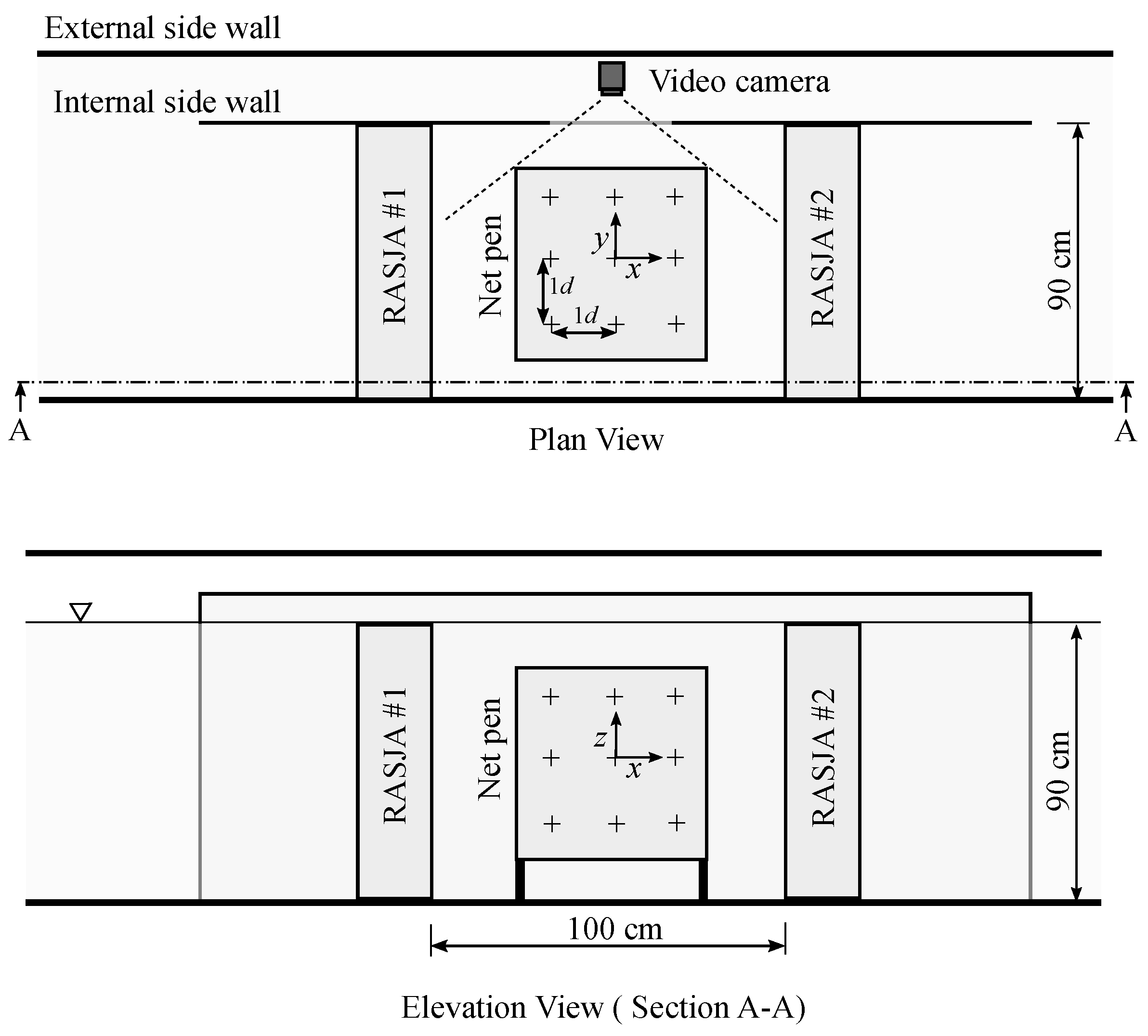
The turbulence test facility was developed at the Aquatic Research Laboratory (ARL) at the Pacific Northwest National Laboratory (PNNL), Richland, WA, USA, and installed in a fiberglass flume measuring 1.2 m wide, 1.4 m deep, and 12.2 m long. An internal wall was installed with a transparent acrylic window to allow underwater video observation of the test section as shown in Figure 1. Fish behavior during the acclimation, test, and post-test was monitored using a high-sensitivity wide-angle low-light monochrome video camera (Deep Sea Wide-i SeaCam) and monitor located in an office trailer.
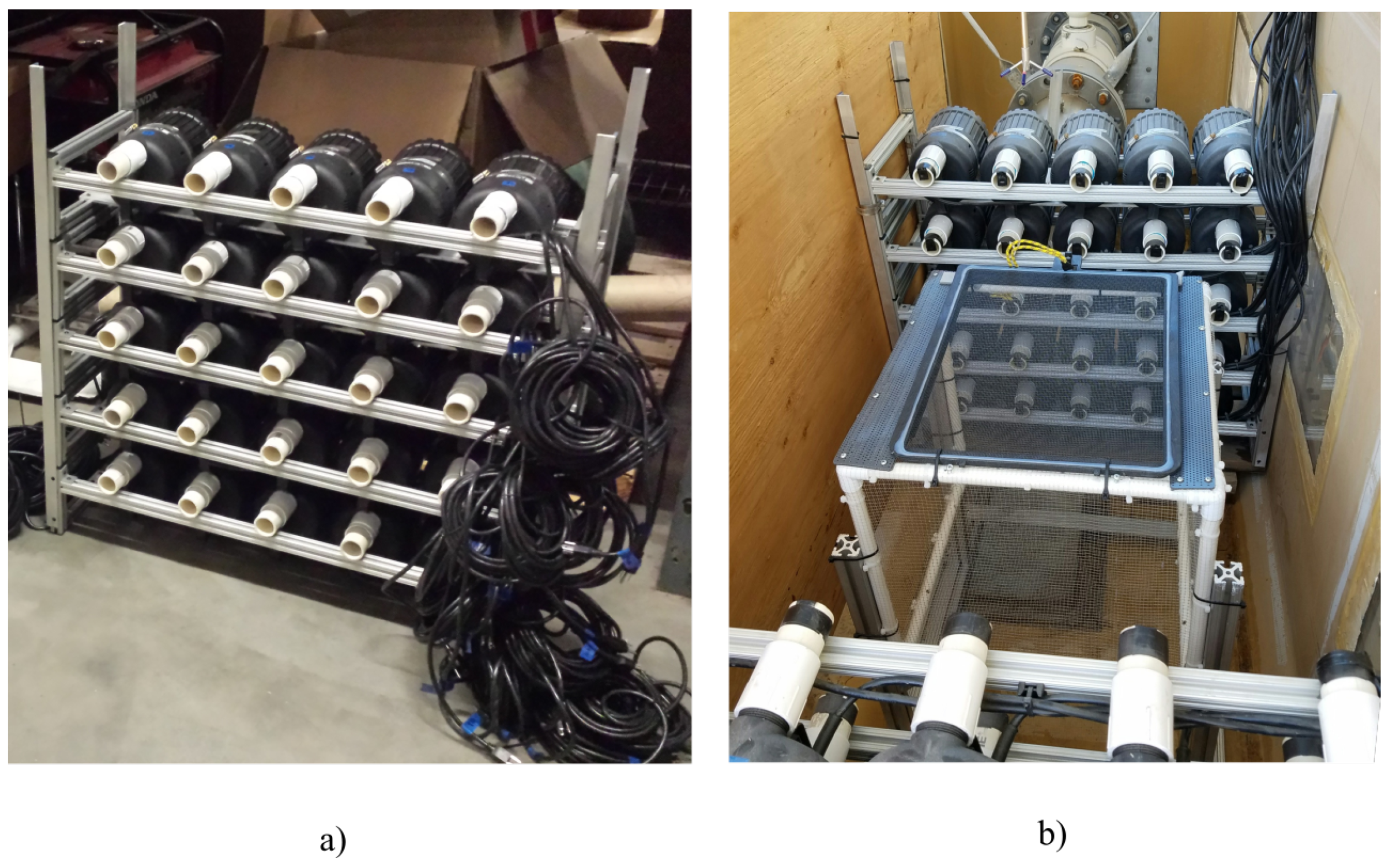
Each RASJA consisted of 25 submersible electric pumps mounted in a array, as shown in Figure 2a. The pump spacing, d, was 160 mm in both the vertical and transverse directions. Thermoplastic utility pumps manufactured by Flotech (Model FP0S3000X) were selected to provide the largest flow rate within the available power limits of the laboratory, with a rated flow rate of 3.15 L/s through a 35-mm diameter nozzle. The discharge rate of all 50 pumps was measured experimentally and had a mean of 2.74 L/s and a standard deviation of 0.08 L/s, which corresponded to a nominal jet exit velocity of 2.84 m/s. These pumps were oil free to avoid contaminating the water during fish testing. The intake to the pump is located at the opposite end of the casing from the nozzle. In this way, the pump intake and outlet are along the same axis and their proximity approximates a synthetic jet configuration. The switching of the pump operation was controlled using LabVIEW (National Instruments) and triggered using a Measurement Computing USB-DIO96 digital output card.
The test volume was defined by a net pen to contain the test fish during each experiment. This was constructed from 25.4 mm PVC pipe framing and clear monofilament mesh netting that had a 6.35 × 6.35 mm square aperture to allow penetration of the turbulent flow into the test section. The net pen was 60 cm long × 45 cm wide × 60 cm deep (Figure 2b). The mesh hole size of the netting was selected to be the large enough to minimize flow interference, while preventing the fish from escaping. All velocity characterization was performed by removing the top lid and measuring the flow within the net pen to account for any flow interference effects induced by the mesh walls.
The firing algorithm of each individual pump was governed by a random selection of on and off times, which were defined by a normal probability distribution with a user-defined mean, , and standard deviation, . The utilization ratio, , describes the proportion of the time that each pump is activated, where .
2.3. Fish Testing
Spring Chinook salmon (Oncorhynchus tshawytscha) eggs were obtained from the Washington Department of Fish and Wildlife, Leavenworth Hatchery (Leavenworth, WA, USA). The eggs were hatched and juvenile salmon were reared indoors at the PNNL ARL in 650 L circular tanks (122 cm diameter × 91 cm depth) supplied with flow-through (set to 23 L/min) Columbia River water (UV-treated and sand-filtered) at ambient river temperature (approximately 17 C). Dissolved oxygen levels were measured using a YSI portable O meter prior to each fish tested and maintained between 8−10 mg/L. Fish experienced a natural photoperiod simulated with fluorescent lighting. The juveniles were fed an ad libitum daily ration of commercial salmon feed (crumble—1.2 mm pellet; Bio Vita Fry, Bio-Oregon, Longview, WA, USA), except for 24 h before testing when fish were unfed. Two weeks prior to the study, fish were graded to size and stocked into five 650 L circular tanks, with the same environmental conditions as those during rearing. The size distribution of fish used in this study ranged from 57–84 mm fork length and 2.7–7.45 g in weight.
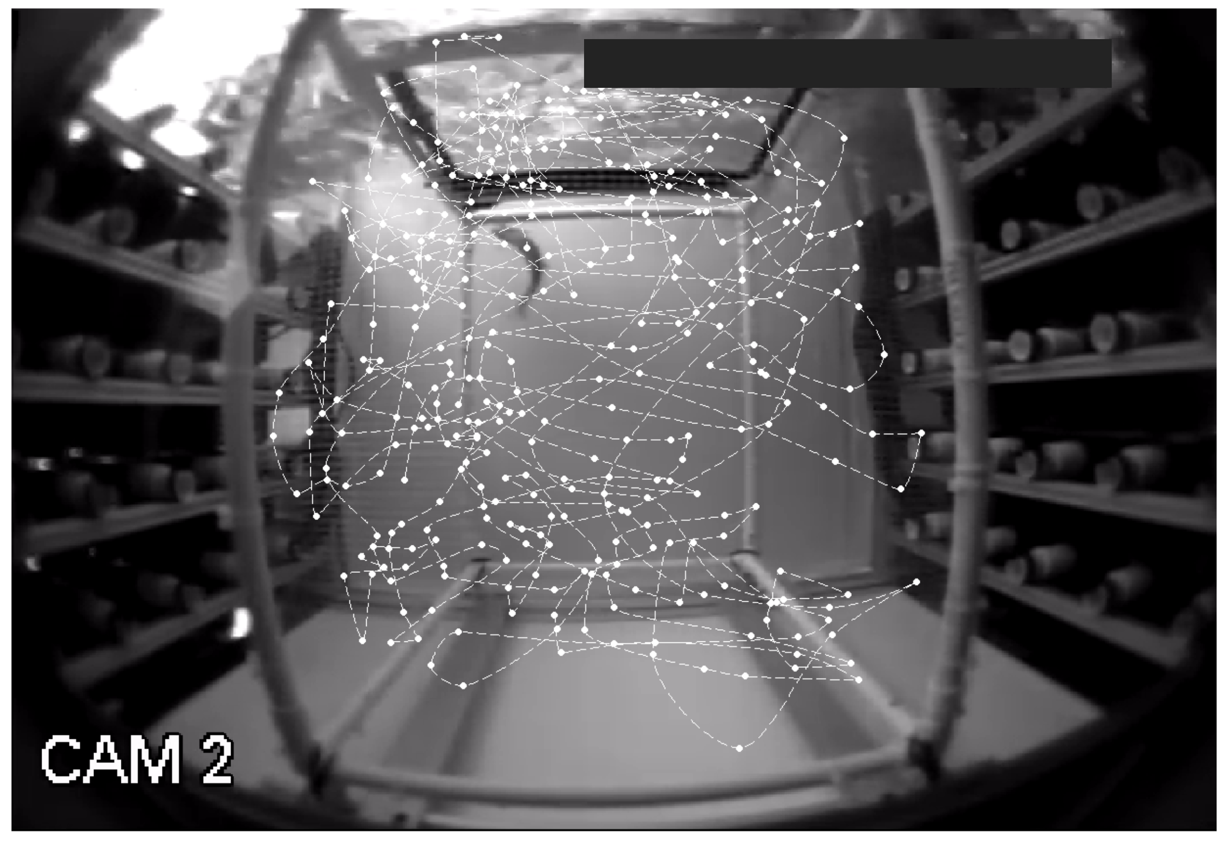
Individual fish were visually inspected for descaling and any other physical defects before being transferred into the net pen. The net pen lid was then secured to prevent the test fish from escaping. Fish were allowed a 10-min acclimation period prior to exposure to turbulence. During this time, fish were observed to monitor their general location within the cage and swimming behavior, as shown in Figure 3. A steady flow condition was generated using a single 10 pumps from RASJA during the acclimation period to create a consistent velocity profile within the net pen for the fish to orientate toward.
Once the acclimation period was completed, the RASJA were used to generate the turbulent flow conditions. Exposure durations of 2 min and 10 min were tested. A total of 49 or 50 fish were tested at each duration, and a randomized schedule of test and control fish was established prior to commencing testing. Control fish were treated the same as test fish except during the exposure period when the pumps were used to generate steady flow conditions identical to the acclimation flow rather than turbulence. Once the exposure time was completed, steady flow was again generated to observe fish recovery behavior. Fish were observed to determine: (1) if they could equilibrate in the water column, (2) if so, the time to reach equilibrium, (3) if they could orient themselves to swimming upstream into the steady flow, and (4) if so, the time to achieve reorientation. The time to reach equilibrium was measured as the time from the end of the turbulence exposure to when the fish was able to maintain a constant vertical position in the net pen. The time to achieve orientation was measured as the time from the end of the turbulence exposure to the time the fish oriented into the steady flow conditions. These results were a subjective assessment by the observer, and observer bias was accounted for through confirmation of identical response assessments in preliminary tests. Fish were then netted out of the net pen, anesthetized, weighed, and measured for fork length and given a unique fin clip to distinguish individuals. Both test and control fish were held for 24 h to assess any post-treatment mortality. An assessment of descaling was conducted at the time of fin clipping and again at the end of the holding period (post-test).
3. Results
3.1. Velocity Characterization
The flow velocity in the test volume was characterized using a Nortek Vectrino+ acoustic Doppler velocimeter (ADV). The tank was seeded using fine natural sediment particles. The seeding material was selected in preference to typical glass microsphere products because the tank drain discharged into a waterway without sufficient filtration to remove non-biodegradable material of that scale. Neutral buoyancy of the seeding particles was achieved by mixing the sediment particles with fresh water and allowing it to settle for a period of 5 min. Any buoyant material was removed from the surface of the settling tank, and then the seeded water was decanted from the mid-portion of the tank.
While the mean velocity can be determined from sampling periods of less than 60 s, higher order velocity metrics such as turbulence velocities require data acquisitions of significantly longer durations [18,23]. For each characterization acquisition, the ADV was set to collect data at 100 Hz for a period of 20 min, with a transmit length of 1.2 mm and a nominally cylindrical sampling volume with a diameter of 6.0 mm and length of 4.9 mm. A nominal velocity range of 2.5 m/s was selected to provide a measureable velocity range of 0.94 m/s and 3.28 m/s in the vertical and horizontal directions, respectively. For further information about the definition and implications of these settings refer to the Nortek User Manual [24].
The velocity signal was filtered using a correlation threshold, a signal-to-noise ratio threshold [25], and phase space filtering [26,27], as summarized in Table 1. The Doppler noise component was then calculated and removed from each velocity component [23].
3.1.1. Effects of Pump Utilization
A range of pump utilization ratios were tested prior to fish testing using mean activation periods from = 0.5 s and = 4 s. These measurements were made at the origin (centroid) of the net pen, as defined by the coordinate system shown in Figure 1. The measured turbulence kinetic energy was in the range of . Preliminary fish tests showed that pump activations of s resulted in fish impact and impingement against the walls of the net pen. For this reason, the selected utilization ratio was with = 1.0 s and = 0.1 s.
3.1.2. Spatial Characterization of Selected Pump Settings
The location of the centroid of the test volume was used for preliminary characterization of the velocity fluctuations. However the unconstrained and unanesthetized test fish were free to inhabit any location within the net pen between the RASJAs. For this reason, it was important to quantify the spatial sensitivity of the fluctuating velocity characteristics.
A 3D array of survey points was established to quantify the velocity fluctuations within the test volume. The survey array had a total of N = 27 points with a unit spacing of , and the center of the survey corresponded to the centroid of the test volume. The survey grid is indicated with cross-hairs in Figure 1. The flow parameters were measured for all 27 surveyed locations. The results are presented for the centroid location as well as the mean, standard deviation (STD) and range of these values over the 27 measured survey points in Table 2. The level of kinetic energy per unit mass associated with the velocity fluctuations, k, is related to the turbulent velocity, , through the relationship of .
The turbulence kinetic energy per unit mass at the centroid was equal to and the mean turbulence energy of all 27 survey locations was . This represents an increase in turbulence kinetic energy by two orders of magnitude compared to previous dual RASJA configurations [19].
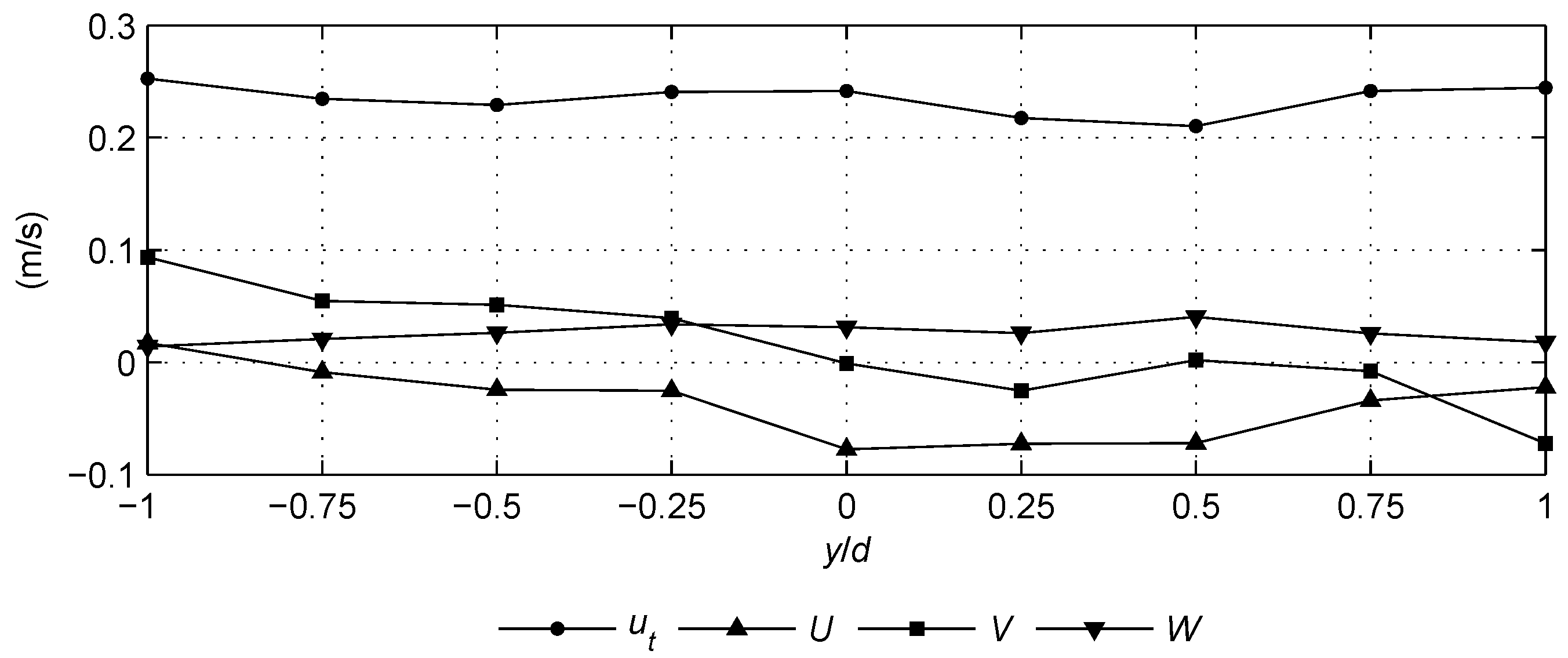
A transverse transect of measurements was taken at the mid-plane () and mid-depth () of the net pen, in increments of . The transverse profile of calculated from this transect is presented in Figure 4. The influence of the jets at , , and can be observed as local maxima in the turbulence profile. The mean turbulent velocity in the profile is 235 mm/s, which agrees closely with the results observed in the velocity survey presented in Table 2.
3.2. Biological Response
A total of 199 juvenile Chinook salmon were used in this experiment. The average size of the fish was 74.6 mm and 7.8 g. Fish from the 2-min turbulence treatment group were significantly longer than fish from the 2 min-control treatment group (Kruskall-Wallis H = 8.453; ). However, there were no significant differences in the mass of fish among treatment groups (Kruskall-Wallis H = 4.553; ; Table 3).
All fish from all exposure treatment groups immediately regained equilibrium after the treatment period ended. There were some delays in the fish’s ability to reorient in steady flow (Table 3). For all exposure treatments, the majority of fish reoriented to steady flow in less than 5 seconds. Twenty-six percent (n = 13 of 49) of the fish exposed to the 10-min turbulence treatment required at least 5 s to reorient themselves in steady flow; however, this was not significantly different than any other treatments (; ). During the initial activation of the RASJA for the turbulent flow test, the general fish behavior included movement back and forth within the width of the net pen, as shown in Figure 3. Test fish were occasionally observed being impinged at the side of the mesh cage during the exposure, but the durations of impingement were less than 2 seconds. Observed fish behavior in the net pen did not indicate any evidence of significant zones of low turbulence.
4. Discussion
Turbulence in stream habitats occurs naturally and is important for a number of processes including predator-prey dynamics [28], swimming speed [29], and habitat selection [30]. A full dose response relationship will require the scaling up of the dual RASJA configuration to generate the representative peak turbulence intensities expected during fish passage through a hydropower facility. Such intensities were not achieved in this set of experiments, because the pump capacity was constrained by the available power limits of the laboratory. The significance of the RASJA approach demonstrated in this work is that the turbulence intensity can be scaled while maintaining a relatively low mean flow velocity. The mean flow velocity can be maintained at a magnitude significantly less than the fluctuating component because the mean discharge of each RASJA is equal in magnitude and opposite in direction. Specifically, the 27-point survey of the net pen showed a mean streamwise, transverse, and vertical bulk velocity of 13.9 mm/s, 0.8 mm/s, and 4.3 mm/s, respectively, while the RMS velocity fluctutations in these directions were 336 mm/s, 190 mm/s, and 167 mm/s, respectively. This is critical in allowing the test fish to remain in the characterized flow volume and be observed throughout the experiment without impingement, regardless of the exposure duration selected.
In these experiments, juvenile Chinook salmon were exposed to turbulent flow conditions and evaluated for survival and behavioral effects. Overall, no significant differences in survival, loss of equilibrium, or time to reorient to steady flow were observed for the test conditions; however, trends observed in the data indicated that longer exposure to the turbulent conditions increased the amount of time that fish needed to reorient themselves in steady flow.
The occurrence of abrasion in laboratory-based turbulence testing has been previously documented. Odeh et al. [4] observed 10% mortality rates in hybrid bass exposed to turbulent conditions and these fish also had up to 37% descaling from abrasion of fish against the walls of their turbulence tank. The authors of that study were unable to determine whether the mortality was due to turbulence or impingement. Such injuries were not observed in these experiments, because the opposing RASJA configuration provided opposing jet arrays from both ends of the net pen. There is a clear trade-off between (a) ensuring the exposure to the turbulent conditions by using a net pen or other structure to limit the fish’s ability to move to areas of refuge and (b) minimizing the fish’s contact with the structure and the consequent abrasion. This is particularly important in studies such as this one where the objectives are to isolate the effects of turbulence from other hydraulic stressors. It follows that this novel approach to creating a turbulent environment for biological testing offers advancement over previously used devices, particularly for simulating hydroturbine passage conditions.
Trends in the behavioral response of juvenile Chinook salmon to the increasing durations of turbulence were suggested, but these differences were not significant. Fish exposed to the 10-min turbulence treatment took longer to reorient themselves in steady flow than those exposed to the 2-min turbulence treatment and the control fish. The inability to become reoriented in steady flow can influence delayed or indirect survival of fish passing through turbine environments [2], because disoriented fish may be more likely to come in contact with structures within the turbine or to be preyed upon in the tailrace. The motion of all fish exposed to the turbulence magnitudes generated in this study was observed to be independent of the direction of the fish, and therefore unlikely to be the result of volitional movement; however, they regained orientation quickly once the turbulence stopped and steady flow resumed.
Because the response of fish to orient themselves into steady flow lagged up to 5 s, the authors considered any time less than 5 seconds to not be biologically significant. All other times were rounded up to the nearest 5-second interval, so final data were binned to those levels. The biological response to the turbulence stressor can be interpreted with improved statistical power by using the measured reorientation time rather than the binned data, and this approach is recommended for future studies.
In a turbine environment, fish may interact with structures during passage (e.g., turbines, draft tube walls), but this study was focused on measuring the effects of turbulence itself and not the interaction of turbulence and collision. Outputs from the Sensor Fish device developed at PNNL [31] and deployed at Ice Harbor Dam on the Lower Snake River, show rotational velocity approaching 1600/s in the draft tube section and decreasing to a maximum of approximately 1000/s in the immediate tailrace [32]. The duration of these rotational velocities for a typical Sensor Fish passing through the blades, draft tube, and into the tailrace section was approximately 2 min, which corresponds to the lower exposure duration of the turbulence tests presented herein.
5. Future Work
The intensity of turbulence generated in this version of the facility was less than the peak intensities expected during dam passage and future studies will aim to increase the magnitude of the turbulence to levels that represent a higher proportion of those experienced during turbine passage. It was assumed that lower turbulence intensity would require longer exposure periods to create an observable biological response. The ability to subject the test fish to extended turbulence exposure without impingement was therefore explored through the selection of 2 min and 10 min durations. Future work is recommended to explore the possibility to increase the turbulence intensity through higher pumping capacity, as well as a range of different exposure durations.
The characterization of the complex turbulent flows within the net pen was limited by the use of a single acoustic Doppler velocimeter in these tests. A single ADV collects a point velocity measurement and in the absence of a mean flow velocity, required for the implementation of Taylor’s frozen turbulence hypothesis, these data are unable to be processed to give any spatial description of the flow structure. For future research the measurement of the spatio-temporal behavior of the flow in the net pen, using methods such as particle image velocimetry or multiple simultaneous point velocity measurements, is recommended to describe the turbulent flow structures in more detail.
The dose-response observations focused on the ability for fish to demonstrate equilibrium and reorientation into a steady state flow following their exposure to turbulence. Ongoing work should also focus on the susceptibility of predation during the turbulence event, because such susceptibility may be more realistic for fish passing through turbines and in the immediate downstream tailrace environment. Variability in the effects on yearling and sub-yearling salmonids is also an area of useful further research, because fish size (in relation to surface area) and mass may be contributing factors in potential injury or descaling in turbulent flow fields.
6. Conclusions
The dual RASJA system developed in this work has been successfully scaled up from previous applications to generate a turbulence field with a turbulence kinetic energy per unit mass of . This represents an increase in turbulent kinetic energy from previously published dual RASJA configurations by two orders of magnitude. The high turbulence levels generated in such a low mean velocity field make the turbulence test facility presented a novel test facility for conducting dose-response experiments to determine the effects of turbulence on fish, because it features the ability to control the exposure and turbulence level in a controlled test volume. The resulting turbulence field allowed for the testing of fish in turbulent conditions without introducing significant impingement or impact, which has obscured results of previous turbulence studies.
The level of turbulence generated in the experiments presented was exceeded in less than 50% of the travel time from the inlet to the draft tube exit in the typical Kaplan turbine operating conditions modeled with CFD simulations. The turbulence of this magnitude did not affect the immediate survival or behavior at either the 2-min or 10-min exposure durations. During the exposure, all fish lost the ability to orient themselves into the flow and maintain a position in the water column, but regained this ability within 5 s in nearly all tests (94%).
Future testing is required to better understand the complete dose response of the turbulence stressor on fish behavior and survival. This will require the development of the RASJA configuration to use larger pumps that can generate increased flow disturbances that approach the maximum expected turbulence intensities during fish passage. The susceptibility to predation, both during and after exposure, is also of interest in future turbulence response experiments.
Author Contributions
Funding acquisition, M.C.R.; conceptualization, M.C.R. and S.F.H.; methodology, M.C.R., S.F.H., A.H.C., P.R.-G. and R.P.M.; investigation, S.F.H. and R.P.M.; writing—original draft, S.F.H.; writing—review and editing, M.C.R., S.F.H., A.H.C., P.R.-G. and R.P.M. P.R.-G. contributed to this research as a PNNL staff member prior to becoming staff member at Andritz Hydro.
Funding
This research was conducted under the Laboratory Directed Research and Development Program at Pacific Northwest National Laboratory, a multi-program national laboratory operated by Battelle for the U.S. Department of Energy.
Acknowledgments
The authors thank Christina MacMillan, Briana Rhode and Trevor Macduff for their assistance with constructing the RASJAs used in these experiments and Ryan Harnish for the statistical design of the experimental procedure. PNNL is accredited by the Association for Assessment and Accreditation of Laboratory Animal Care. Juvenile salmon were handled in accordance with federal guidelines for the care and use of laboratory animals, and the protocols for our study were conducted in compliance with and approved by PNNL’s Institutional Animal Care and Use Committee.
Conflicts of Interest
The authors declare no conflict of interest.
Abbreviations
The following abbreviations are used in this manuscript:
| ADV | acoustic Doppler velocimeter |
| ARL | Aquatic Research Laboratory |
| CFD | computational fluid dynamics |
| cfs | cubic feet per second |
| hp | horse-power |
| L | liter(s) |
| LDV | laser Doppler velocimeter |
| MW | megawatt(s) |
| PNNL | Pacific Northwest National Laboratory |
| PVC | polyvinyl chloride |
| RASJA | randomly actuated synthetic jet array |
| RMS | root-mean square |
| STS | submersible traveling screen |
| USACE | U.S. Army Corps of Engineers |
| VBS | vertical barrier screen |
Appendix A. Computational Estimate of Turbulence Exposure During Dam Passage
The selected Kaplan turbine unit is located at Ice Harbor Dam, which is operated by the U.S. Army Corps of Engineers (USACE) Walla Walla District on the Snake River, WA, USA. A detailed description of the site and the geometry model provided by the USACE are available in the publicly accessible report by Harding et al. [21]. Computational fluid dynamics (CFD) was applied to numerically solve the continuity equations for mass and momentum over the discretized volume contained within the geometry. The commercial CFD software Star-CCM+ Version 10.06 [22] was used for mesh generation and flow simulations.
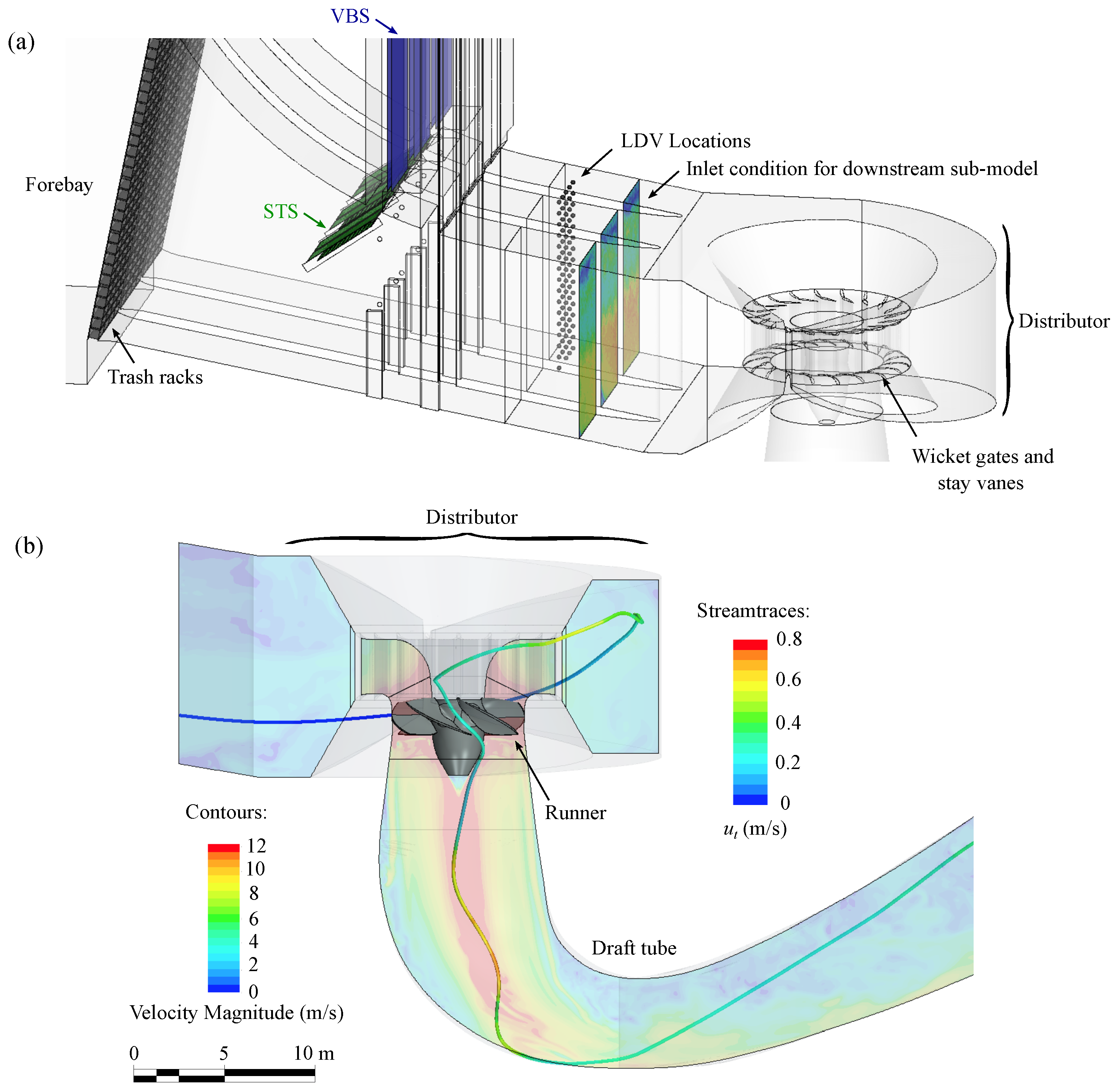
The entire domain was divided into two sub-models; the upstream and downstream regions, shown in Figure A1a,b, respectively. The upstream model included a portion of the forebay, trash racks, submersible traveling screens (STS), vertical barrier screens (VBS), distributor, and flow direction-controlling structures (stay vanes and wicket gates). The downstream model was also comprised of the distributor and flow direction-controlling structures, as well as the runner and the draft tube. These elements of the hydroturbine are annotated in Figure A1. The distributor therefore constituted an overlapping portion that allowed us to describe intake flows that supplied the precursor inflow conditions for the downstream passage section. Using a precursor CFD simulation to generate inflow conditions for domains farther downstream is a common practice in research and industry studies of fluid flows in complex geometries. Note that the STS and VBS structures are part of the bypass system designed to divert a portion of the fish entering the turbine from passing through the turbine runner.
While the computational modeling of hydroturbine flows has a long history in industry and research-oriented work, the present approach differed from most preceding studies in two aspects. First, the temporally and spatially dependent velocity and pressure components were solved at the prototype scale and at high spatio-temporal resolution by means of eddy-resolving turbulence modeling techniques. The usual practice is to apply turbulence-averaging techniques at steady state, which is efficient and accurate for calculating mean flow fields in reduced-scale geometries but not for computing turbulence fields (e.g., turbulent kinetic energy and its rate of dissipation) at the prototype scale.
Second, the validation was conducted by means of acceptable comparisons between the modeling results and either the corresponding reduced-scale physical model or full-scale field data. The CFD velocities in the upstream model were compared with experimental velocities measured within a reduced-scale model of the turbine geometry. The reduced-scale experimental velocities were measured using laser Doppler velocimetry (LDV) at the location shown in Figure A1a and scaled up using Froude scaling to compare with the full-scale values [20,21,33]. To the best of our knowledge, the aforementioned features have not been simultaneously implemented in the modeling of flow in a complete turbine system. Flow data were not available for the downstream model, but USACE provided plant estimates of the power and discharge at the selected operating point (USACE, Personal Communication). The field estimate for shaft power was 103.20 MW (138,400 hp) and the corresponding CFD-based shaft power was 101.14 MW (135,628 hp), which lie within an acceptable error considering the intrinsic limitation of the modeling approach to represent the flow physics. Similarly the field estimate of discharge was 379.45 (13,400 cfs), which agreed with that of the CFD model (386.36 ) to within 2%.
Figure A1.
The turbine intake geometry divided into (a) an upstream model and (b) a downstream model. The upstream model is annotated to show the locations of the trash racks for debris collection, submersible traveling screens (STS) and vertical barrier screens (VBS) for fish diversion around the powerhouse, and the locations of the laser Doppler velocimetry (LDV) measurements used in model validation. The location of the inlet conditions used in the downstream model is also indicated. The velocity contour indicates the flow speed in cross-sectional plane of the downstream model. The path of a single streamtrace is also shown for this model to indicate the variation in turbulence velocity during turbine passage.

Contour plots of instantaneous velocities at the upstream and downstream sub-models are shown in Figure A1. Figure A1a includes the location of laser Doppler velocimetry (LDV) where mean and RMS velocity data were measured in a 1:25 reduced-scale physical hydraulic model at USACE’s Engineering Research and Development Center.
The upstream and downstream sub-models were discretized into 127.5M and 134.5M hexahedral cells, respectively. In both cases, the convection terms were selected as 2nd-order upwind/central schemes for the detached eddy version of the SST turbulence model [34]. For details about the time step, mesh and boundary conditions, refer to Romero-Gomez and Richmond [20].
The behavior of fish before and during turbine passage is the subject of some uncertainty among biologists. Of significance to turbine passage is the observation that juvenile salmon tend to orient themselves with their heads upstream in the turbine intake [35]. However, observation of fish beyond the intake has not been possible [36], so their behavior and their paths have never been measured. This knowledge gap has led many researchers to assume that fish basically follow the flow when confronted with the high velocities of the turbine environment [37]. This is substantiated by the observation that the burst speed of juvenile salmon does not exceed about nine body-lengths per second [38], or about 1 m/s, which is significantly lower than the 5–20 m/s velocities typical of the turbine environment. As such, the velocity of the fish relative to the flow velocity is assumed to be zero in this study. Thus, was selected as the quantity to describe and examine turbulent conditions in both the numerical and experimental phases of the present work.
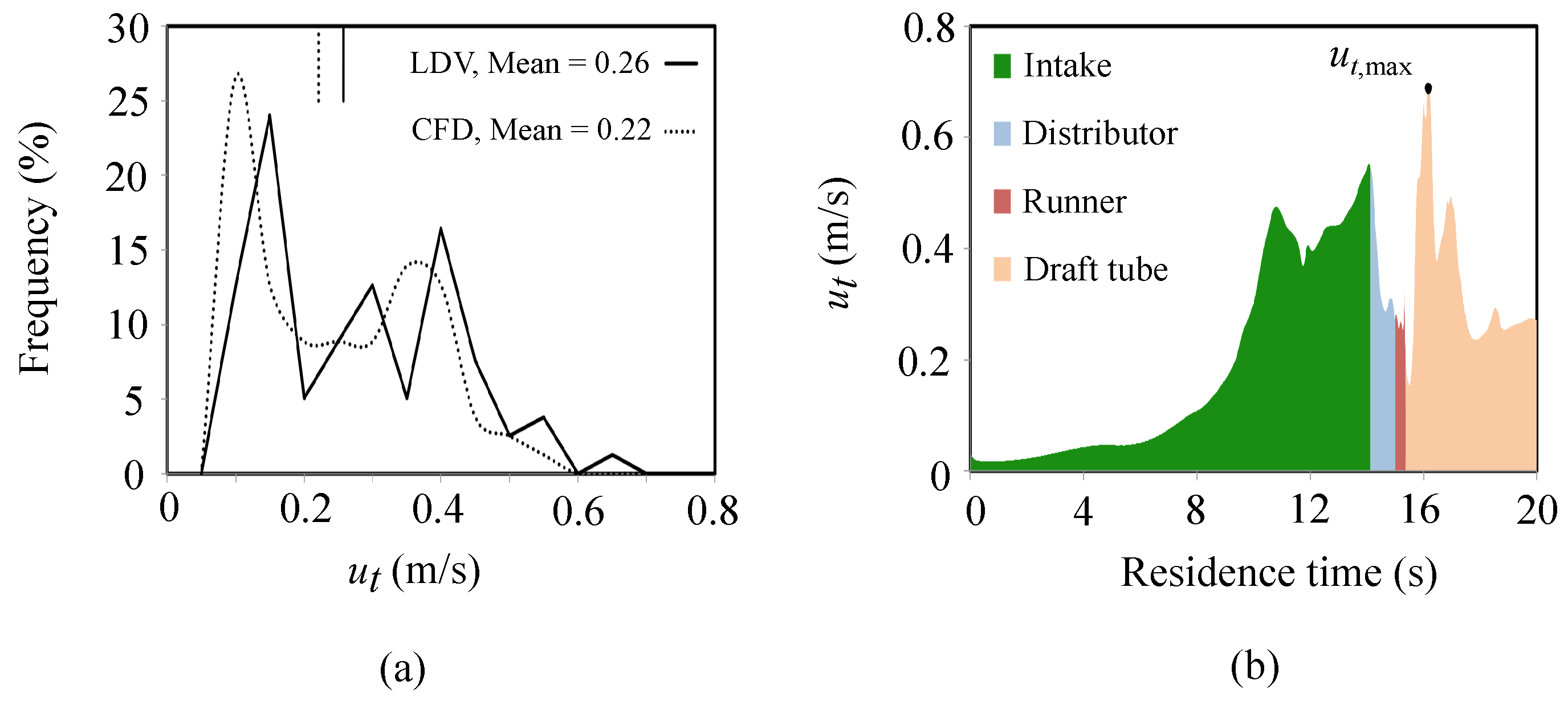
Figure A2a compares both LDV and CFD results and shows that an average of m/s can be considered a prevalent turbulent condition within the intake. The main source of flow variability arises from the flow blockage effect of the deployed STSs. Retracting the STS is the preferred configuration during the months of the year when no fish migration is observed and significantly reduces the turbulence at the intake (for results from the “No STS” configuration see Harding et al. [21]). In the downstream section (Figure A1b), the prevailing turbulence conditions were examined by sampling along streamtraces. Figure A2b shows the variability of as a function of residence time in a way similar to how a fish would encounter it during passage. The turbulence increases as the streamtrace travels through the scroll case, but it begins to decrease gradually through the distributor and the runner. This turbulence decay as a result of the geometric contraction has been widely studied (e.g., [39]). The entrance to the draft tube is accompanied by increasing turbulence owing to strong inlet swirl, runner blade wakes, and expansion of the flow. Turbulence and flow separation are phenomena that designers typically work to minimize in draft tube design in an effort to enhance hydraulic efficiency. The maximum value of turbulence indicated in Figure A2b is usually located at the draft tube.
Approximately 1000 streamtraces were seeded in a distribution that covered the intake beneath the VBS gate slot. These were generated with the averaged flow velocities and sampled along each trajectory to collect a statistically meaningful description of . The residence time refers to the length of time that a particle following the streamtrace has traveled since its inception in the intake.
Figure A2.
Comparison of (a) from LDV and CFD in upstream model and (b) the time series of that fish could potentially encounter, calculated using one thousand streamtraces.
Figure A2.
Comparison of (a) from LDV and CFD in upstream model and (b) the time series of that fish could potentially encounter, calculated using one thousand streamtraces.

While the shaft power and discharge modeled by the CFD were seen to match those of the field estimate, there are no available data for the verification of the turbulence values in the downstream model. However it is apparent that the turbulence velocities calculated using this CFD approach are comparable to other experimental work on the subject (e.g., [4]).
References
- Therrien, J.; Bourgeois, G. Fish Passage at at Small Hydro Sites; Technical Report; Genivar Consulting Group for CANMET Energy Technology Centre: Ottawa, ON, Canada, 2000. [Google Scholar]
- Čada, G.F. The development of Advanced Hydroelectric Turbines to Improve Fish Passage Survival. Fisheries 2001, 26, 14–23. [Google Scholar] [CrossRef]
- Lacey, R.; Neary, V.S.; Liao, J.C.; Enders, E.; Tritico, H.M. The IPOS framework: Linking fish swimming performance in altered flows from laboratory experiments to rivers. River Res. Appl. 2012, 28, 429–443. [Google Scholar] [CrossRef]
- Odeh, M.; Noreika, J.F.; Haro, A.; Maynard, A.; Castro-Santos, T.; Cada, G.F. Evaluation of the Effects of Turbulence on the Behaviour of Migratory Fish; Final Report 2002, Report to Bonneville Power Administration, Contact No. 00000022, Project No. 200005700; Oak Ridge National Laboratory (ORNL) and US Geological Survey (USGS): Oak Ridge, TN, USA; Reston, VA, USA, 2002; p. 55.
- Neitzel, D.A.; Dauble, D.D.; Cada, G.F.; Richmond, M.C.; Guensch, G.R.; Mueller, R.R.; Abernethy, C.S.; Amidan, B. Survival estimates for juvenile fish subjected to a laboratory-generated shear environment. Trans. Am. Fish. Soc. 2004, 133, 447–454. [Google Scholar] [CrossRef]
- Silva, A.; Santos, J.; Ferreira, M.; Pinheiro, A.; Katopodis, C. Effects of water velocity and turbulence on the behaviour of Iberian Barbel (Luciobarbus bocagei, Steindachner 1864) in an experimental pool-type fishway. River Res. Appl. 2011, 27, 360–373. [Google Scholar] [CrossRef]
- Trinci, G.; Harvey, G.L.; Henshaw, A.J.; Bertoldi, W.; Hölker, F. Life in turbulent flows: Interactions between hydrodynamics and aquatic organisms in rivers. Wiley Interdiscip. Rev. Water 2017, 4, 1–16. [Google Scholar] [CrossRef]
- Ryon, M.G.; Cada, G.F.; Smith, J.G. Further Tests of Changes in Fish Escape Behavior Resulting from Sublethal Stresses Associated with Hydroelectric Turbine Passage; Technical Report; Oakridge National Laboratory: Oak Ridge, TN, USA, 2004. [CrossRef]
- Roach, P. The generation of nearly isotropic turbulence by means of grids. Int. J. Heat Fluid Flow 1987, 8, 82–92. [Google Scholar] [CrossRef]
- Cheng, N.; Law, A. Measurement of turbulence generated by oscillating grid. J. Hydraul. Eng. 2001, 127, 201–208. [Google Scholar] [CrossRef]
- Srdic, A.; Fernando, H.; Montenegro, L. Generation of nearly isotropic turbulence using two oscillating grids. Exp. Fluids 1996, 20, 395–397. [Google Scholar] [CrossRef]
- Stiansen, J.; Sundby, S. Improved methods for generating and estimating turbulence in tanks suitable for fish larvae experiments. Sci. Mar. 2001, 65, 151–167. [Google Scholar] [CrossRef] [Green Version]
- Knebel, P.; Kittel, A.; Peinke, J. Atmospheric wind field conditions generated by active grids. Exp. Fluids 2011, 51, 471–481. [Google Scholar] [CrossRef]
- Makita, H. Realization of a large-scale turbulence field in a small wind tunnel. Fluid Dyn. Res. 1991, 8, 53–64. [Google Scholar]
- Mydlarski, L.; Warhaft, Z. On the onset of high-Reynolds-number grid-generated wind tunnel turbulence. J. Fluid Mech. 1996, 320, 31–68. [Google Scholar] [CrossRef]
- Maia, A.; Sheltzer, A.; Tytell, E. Streamwise vortices destabilize swimming bluegill sunfish (Lepomis macrochirus). J. Exp. Biol. 2015, 218, 786–792. [Google Scholar] [CrossRef]
- Variano, E.A.; Bodenschatz, E.; Cowen, E.A. A random synthetic jet array driven turbulence tank. Exp. Fluids 2004, 37, 613–615. [Google Scholar] [CrossRef]
- Variano, E.A.; Cowen, E.A. A random-jet-stirred turbulence tank. J. Fluid Mech. 2008, 604, 1–32. [Google Scholar] [CrossRef]
- Bellani, G.; Variano, E.A. Homogeneity and isotropy in a laboratory turbulent flow. Exp. Fluids 2014, 55, 1646. [Google Scholar] [CrossRef]
- Romero-Gomez, P.; Richmond, M.C. Movement and collision of Lagrangian particles in hydro-turbine intakes: A case study. J. Hydraul. Res. 2017, 55, 706–720. [Google Scholar] [CrossRef]
- Harding, S.; Romero-Gomez, P.; Richmond, M. Performance of Virtual Current Meters in Hydroelectric Turbine Intakes; Technical Report; Pacific Northwest National Laboratory: Richland, WA, USA, 2016.
- CD-adapco. User Guide, STAR-CCM+ Version 10.06; CD-adapco; Siemens PLM Software: Plano, TX, USA, 2015. [Google Scholar]
- Hurther, D.; Lemmin, U. A correction method for turbulence measurements with a 3D acoustic Doppler velocity profiler. J. Atmos. Ocean. Technol. 2001, 18, 446–458. [Google Scholar] [CrossRef]
- Nortek, A.S. Vector Current Meter User Manual; Technical Report August; Nortek AS: Rud, Norway, 2005. [Google Scholar]
- Rusello, P.; Lohrmann, A.; Siegel, E.; Maddux, T. Improvements in acoustic Doppler velocimetery. In Proceedings of the 7th International Conference in Hydroscience and Engineering (ICHE 2006), Philadelphia, PA, USA, 10–13 September 2006. [Google Scholar]
- Mori, N. MACE Toolbox. Available online: http://www.oceanwave.jp/softwares/mace (accessed on 19 August 2017).
- Mori, N.; Suzuki, T.; Kakuno, S. Noise of acoustic Doppler velocimeter data in bubbly flow. ASCE J. Eng. Mech. 2007, 133, 122–125. [Google Scholar] [CrossRef]
- Cotal, A.; Webb, P.; Tritico, H. Do brown trout choose locations with reduced turbulence? Trans. Am. Fish. Soc. 2006, 135, 610–619. [Google Scholar] [CrossRef]
- Higham, T.; Steward, W.; Wainwright, P. Turbulence, temperature, and turbidity: The ecomechanics of predator-prey interactions in fishes. Integr. Comp. Biol. 2015, 55, 6–20. [Google Scholar] [CrossRef]
- Lupandin, A. Effect of flow turbulence on swimming speed of fish. Biol. Bull. 2005, 32, 461–466. [Google Scholar] [CrossRef]
- Deng, Z.; Carlson, T.J.; Duncan, J.P.; Richmond, M.C. Six-degree-of-freedom sensor fish design and instrumentation. Sensors 2007, 7, 3399–3415. [Google Scholar] [CrossRef]
- Carlson, T.; Duncan, J.; Deng, Z. Data Overview for Sensor Fish Samples Acquired at Ice Harbor, John Day, and Bonneville II Dams in 2005, 2006, and 2007; Technical Report; Pacific Northwest National Laboratory: Richland, WA, USA, 2008.
- Romero-Gomez, P.; Harding, S.; Richmond, M. The effects of sampling location and turbulence on discharge estimates in short converging turbine intakes. Eng. Appl. Comput. Fluid Mech. 2017, 11, 513–525. [Google Scholar] [CrossRef]
- Spalart, P. Detached-Eddy simulation. Annu. Rev. Fluid Mech. 2009, 41, 181–202. [Google Scholar] [CrossRef]
- Coutant, C.C.; Whitney, R.R. Fish behavior in relation to passage through hydropower turbines: A review. Trans. Am. Fish. Soc. 2000, 129, 351–380. [Google Scholar] [CrossRef]
- Moursund, R.; Carlson, T. Turbine Imaging Technology Assessment; Technical Report; Pacific Northwest National Laboratory: Richland, WA, USA, 2004.
- Weiland, M.; Mueller, R.; Carlson, T.; Deng, Z.; McKinstry, C. Characterization of Bead Trajectories through the Draft Tube of a Turbine Physical Model; Technical Report; Pacific Northwest National Laboratory: Richland, WA, USA, 2005.
- Puckett, K.; Dill, L. Cost of sustained and burst swimming to juvenile Coho Salmon (Oncorhynchus kisutch). Can. J. Fish. Aquat. Sci. 1984, 41, 1546–1551. [Google Scholar] [CrossRef]
- Brown, M.L.; Parsheh, M.; Aidun, C.K. Turbulent flow in a converging channel: Effect of contraction and return to isotropy. J. Fluid Mech. 2006, 560, 437–448. [Google Scholar] [CrossRef]
Figure 1.
Schematic of the dual RASJA test facility showing the window in the internal side wall for underwater surveillance of fish during testing. Locations of the velocity survey are indicated with cross-hairs with a separation of .
Figure 1.
Schematic of the dual RASJA test facility showing the window in the internal side wall for underwater surveillance of fish during testing. Locations of the velocity survey are indicated with cross-hairs with a separation of .

Figure 2.
Implementation of RASJA experiments; (a) Installation of submersible pumps onto racks during the construction of one RASJA, and (b) location of the net pen between the dual RASJA configuration.
Figure 2.
Implementation of RASJA experiments; (a) Installation of submersible pumps onto racks during the construction of one RASJA, and (b) location of the net pen between the dual RASJA configuration.

Figure 3.
Fish track of a representative 2-min turbulence test captured from surveillance video footage. The location of the center of the fish, recorded every 0.3 s, is indicated with a white circle and the interpolated fish track is indicated with a dashed line.
Figure 3.
Fish track of a representative 2-min turbulence test captured from surveillance video footage. The location of the center of the fish, recorded every 0.3 s, is indicated with a white circle and the interpolated fish track is indicated with a dashed line.

Figure 4.
Transect of turbulent velocity, , and mean velocity components (U, V and W) at , , .


Table 1.
Summary of ADV quality control.
| Filter | Threshold | % of Data Rejected |
|---|---|---|
| Correlation threshold | 70% | 33.3 |
| Signal-to-noise ratio threshold | 20 dB | 0 |
| Phase space filtering | - | 0.34 |
Table 2.
Summary of turbulent flow conditions within the surveyed region of the net pen.
| Centroid | Survey Mean | Survey STD | Survey Range | |
|---|---|---|---|---|
| () | () | () | () | |
| U (mm/s) | 151.6 | 438 | ||
| V (mm/s) | 0.8 | 44.1 | 192 | |
| W (mm/s) | 31.3 | 4.3 | 31.0 | 126 |
| (mm/s) | 341.5 | 335.5 | 26.7 | 105 |
| (mm/s) | 183.7 | 190.0 | 8.6 | 35 |
| (mm/s) | 155.2 | 167.0 | 6.9 | 31 |
| (mm/s) | 241.1 | 242.8 | 12.7 | 50 |
| k (m2/s2) | 0.0872 | 0.0887 | 0.0091 | 0.036 |
Table 3.
Summary of juvenile Chinook salmon morphology and reorientation times.
| Exposure Duration | 2 min | 2 min | 10 min | 10 min |
|---|---|---|---|---|
| Exposure Condition | Turbulence | Control | Turbulence | Control |
| Sample size | 50 | 50 | 49 | 50 |
| Median fork length (mm) | 77 | 74 | 75 | 74 |
| Mean fish mass (g) | 4.9 | 4.6 | 4.9 | 4.7 |
| Time to Reorient in Steady Flow (s): | ||||
| <5 | 45 (90%) | 50 (100%) | 36 (74%) | 47 (94%) |
| 5 | 2 (4%) | 0 (0%) | 7 (14%) | 0 (0%) |
| 10 | 3 (6%) | 0 (0%) | 5 (10%) | 3 (6%) |
| 15 | 0 (0%) | 0 (0%) | 1 (2%) | 0 (0%) |
© 2019 by the authors. Licensee MDPI, Basel, Switzerland. This article is an open access article distributed under the terms and conditions of the Creative Commons Attribution (CC BY) license (http://creativecommons.org/licenses/by/4.0/).
Share and Cite
MDPI and ACS Style
Harding, S.F.; Mueller, R.P.; Richmond, M.C.; Romero-Gomez, P.; Colotelo, A.H. Fish Response to Turbulence Generated Using Multiple Randomly Actuated Synthetic Jet Arrays. Water 2019, 11, 1715. https://doi.org/10.3390/w11081715
AMA Style
Harding SF, Mueller RP, Richmond MC, Romero-Gomez P, Colotelo AH. Fish Response to Turbulence Generated Using Multiple Randomly Actuated Synthetic Jet Arrays. Water. 2019; 11(8):1715. https://doi.org/10.3390/w11081715
Chicago/Turabian StyleHarding, Samuel F., Robert P. Mueller, Marshall C. Richmond, Pedro Romero-Gomez, and Alison H. Colotelo. 2019. "Fish Response to Turbulence Generated Using Multiple Randomly Actuated Synthetic Jet Arrays" Water 11, no. 8: 1715. https://doi.org/10.3390/w11081715
Note that from the first issue of 2016, this journal uses article numbers instead of page numbers. See further details here.