Morphological Patterns at River Contractions


School of Engineering, University of Basilicata, Viale dell’Ateneo Lucano 10, I-85100 Potenza, Italy
*
Author to whom correspondence should be addressed.
Water 2019, 11(8), 1683; https://doi.org/10.3390/w11081683
Submission received: 22 July 2019
/
Revised: 8 August 2019
/
Accepted: 12 August 2019
/
Published: 14 August 2019
(This article belongs to the Special Issue Bridge Hydraulics: Current State of the Knowledge and Perspectives)
Abstract
:Sediment transport at river contractions is an important process of engineering concern which might occur when a river encounters a reduction in flow area because of either natural or artificial constraints. This paper focuses on the morphological patterns that are prone to form at and around the constriction of watercourses based on experimental investigations at laboratory scale. Experiments were carried out at the University of Basilicata, Italy, in a 1 m wide and 20 m long rectangular channel. The length of the working section extended up to 16 m, according to the length of the contraction model. Two nearly-uniform sediments were used as mobile bed, sand with median grain size d50 = 1.7 mm and gravel with d50 = 9.0 mm. The contraction length was either 0.5, 1.0, 2.0 or 3.0 m. Runs were carried out under steady flow and clear-water approach flow conditions. Typically, they were of long duration (up to 15 days) also to achieve an equilibrium state. New predictive equations are given on the temporal progress of: the maximum scour depth, the scour hole length, and the axial bed profile with emphasis on the processes of bed aggradation or degradation beyond the contracted region.
1. Introduction
The constriction of watercourses may be induced from natural causes (e.g., landslide debris, development of gravel bars, river junctions), hydraulic structures (like in the emblematic case of bridges), or even from river training works (like in the emblematic case of structures built to obtain greater navigable depths). When the approaching flow is subcritical, the narrowing of rivers involves an increase in flow velocities with possible significant erosional impacts.
Channel contractions are considered long when the flow is nearly uniform in both the undisturbed channel and the contracted reach. According to Komura [1] these conditions arise when the ratio of the contraction length, l, to the approaching channel width, B, is greater than 1, whereas greater than 2 according to Webby [2]. Dey and Raikar [3] substantiate the condition l/B ≥ 1 through an extensive experimental investigation.
In 1934 Straub [4] published a paper on the effects of channel-contraction works upon the regime of movable bed-streams. He suggested a straightforward equation to predict the flow depth in the contracted section based on sediment-discharge and flow-discharge continuity equations. Many formulas, similar in structure to that of Straub, to calculate the maximum scour depth at the equilibrium state, were developed in the second half of 1900 (e.g., Laursen [5], Komura [1], Gill [6], Lim [7], Lim and Cheng [8]). An overview of the most remarkable studies in the 20th century is given in Melville and Coleman [9]. More recently, Briaud et al. [10] extended the SRICOS-EFA (Scour Rate in Cohesive Soils-Erosion Function Apparatus) method to the case of contraction scour. The method addresses clear-water contraction scour in fine-grained soils and is based on site-specific soil testing. An extensive experimental campaign was performed by Dey and Raikar [3] who have used 8 nearly-uniform sediments with d50 from 0.81 mm to 14.25 mm. Experiments were carried out, under clear-water regime, in a 12 m long and 0.6 m wide flume with a uniform contraction zone of 1 m length. Dey and Raikar [11] have developed a semi-theoretical approach to predict the scour depth in long contractions under live-bed approach flow conditions. A satisfactory agreement was found between the model predictions and the experimental data collected by them. These experimental data were also used to verify the reliability of some literature formulas, and the Lim’s [7] formula turned out to be the best. Brandimarte et al. [12] proposed a mathematical model of contraction scour, in unsteady flow and clear-water conditions, to predict the scour depth over the life of the bridge. The model considers the cohesion of the soil.
Bui et al. [13] proposed an artificial neural network (ANN) and an adaptive neuro-fuzzy system (ANFIS), which could accurately estimate the maximum equilibrium depth of the contraction scour. The results showed that the selected networks would estimate the equilibrium maximum scour depth under clear-water conditions significantly better than other conventional methods. The sensitivity analysis revealed the contraction ratio (i.e., the ratio of the contracted channel width to the un-contracted channel width) to be by far the most sensitive parameter, followed by the effect of armor layer formation for non-uniform sediments. Also Raikar et al. [14] emphasize the application of soft computing tools such as ANN and a genetic algorithm (GA) in the prediction of the scour depth within channel contractions. They found that the GA model predicts the maximum scour depth equally well as that of the empirical model of Dey and Raikar [3]. More generally, both ANN and GA models can be satisfactorily used to predict the scour depth within channel contractions. Najafzadeh et al. [15] investigated local scour depth in long contractions of rectangular channels using ANFIS and support vector machines (SVM). The results showed that the developed ANFIS model could predict scour depth more accurately than SVM. Results of sensitivity analysis indicated that the contraction ratio is the most important parameter in modelling of the scour depth by the ANFIS model.
Available experimental data at the field-scale are rather restricted. Surveys of clear-water contraction scour in cohesive soils at bridges in the South Carolina Piedomont are well described in Benedict [16]; Mueller and Wagner [17] have documented real-time measurements for contraction and local scour at two bridges over the Pomme de Terre River in Minnesota during the April 1997 flooding. Hong and Abid [18] used a 1/45 physical scaled-model, considering river bathymetry, to investigate local and contraction scour at Ocmulgee River Bridge, Georgia. A satisfactory agreement was found, in terms of maximum scour depths, when comparing field and experimental data. Interesting field studies on long contraction scour at channels in natural contexts are those by Hayden and Puleo [19] and Li and Zheng [20]. Hayden and Puleo [19] studied bed morphological changes at the Indian River Inlet (DE, USA) that is the only connection between the Atlantic Ocean and Rehoboth and Indian River bays. The present bridge piers within the Indian River Inlet are adjacent to deep scour holes that threaten the bridge. A new scour monitoring system using two three-dimensional profiling sonars was installed on the Indian River Inlet Bridge to observe more than 19,000 m2 of bathymetry daily. Li and Zheng [20] made bed observations along a straight tidal channel using a vessel-based acoustic Doppler current profiler. Observations revealed two scour holes of 25 m deep, separated by 330 m, in and out of an otherwise flat 8 m deep tidal pass leading to the Lake Pontchartrain in southeastern Louisiana in the United States.
However, the available experimental and field data to corroborate the existing predictive models are still limited. More important, the majority of literature studies focuses on the maximum scour depth and dynamic equilibrium conditions, lacking a more detailed characterization of the bed morphology and the effect of time. Finally, it the distinction between short and long contraction, and whether this separation is needed, remain unclear. The present paper aims to provide a contribution to this context. Starting from previous and partial results by the Authors (Oliveto and Marino [21,22], Oliveto [23]), new and definitive equations are drawn up also on the basis of the experimental works by Gill [6], Webby [2], and Dey and Raikar [3]. The proposed time-dependent predictive models would describe to a greater extent the typical bed forms that develop at and downstream of the contracted area.
2. Experiments
Altogether 31 different experiments were conducted at the Hydraulic Engineering Laboratory, University of Basilicata, Italy. A straight channel (with side glass walls) 20 m long and with rectangular cross-section 1 m wide and 1 m deep was used for the experiments.
The mobile bed had 1 m width, 0.5 m height, and from 10 up to 16 m length according to the length of the contraction model. Two bed sediments were used either an almost uniform (in size) sand with median grain size d50 = 1.7 mm, sediment gradation σ = (d84/d16) = 1.5, and dimensionless grain size D* = (g′/ν2)1/3d50 = 43 or an almost uniform (in size) gravel with d50 = 9.0 mm, σ = 1.5, and D* = 228. ν is the kinematic viscosity of water and g′ is the modified gravitational acceleration equal to g(ρs − ρ)/ρ, with g gravitational acceleration, ρs mass density of sediment, and ρ mass density of water. These values of D* (>10) would guarantee transition or turbulent regimes for sediment-water two-phase flows (based on Shield’s diagram). The length of the mobile bed upstream of the beginning of the contraction model was no less than 5 m to allow the development of fully turbulent flows. On the other hand, the length of the mobile bed downstream of the end of the contraction model was no less than 3 m to allow bed aggradation and degradation processes.
Four uniformly contracted reaches of length l either 0.5, 1.0, 2.0, or 3.0 m were considered. Moreover, three contraction ratios β = b/B were studied 0.9, 0.8, or 0.7, with b the width of the uniformly contracted reach and B the width of the undisturbed channel. The upstream contraction inlet and the downstream contraction outlet were identical in shape and triangular (for runs carried out from 2013 until now) or streamlined (for runs carried out in 2004–2005). The ratio of b, and hence of B, to the approach flow depth ho was always kept greater than or close to 5 (except for a couple of runs) to minimize sidewall effects [3,24].
Experimental conditions involved steady flow and clear-water regime. Moreover, the mobile bed at run starting was flat and almost horizontal. The flow discharge was measured using an orifice plate inserted into the supply pipe with an accuracy of ±3%. A conventional point gauge with an accuracy of ±0.1 mm was used to survey the water surface while a so-called shoe gauge, e.g., [21,23] was used for monitoring bed levels. Typically, around 500 bed-level data were collected at the end of each run while about 10–15 measurements only along the channel centreline at the contraction zone and downstream were collected during the run for avoiding disturbances to the flow and bed evolution.
The flow depth in the channel was adjusted by regulating a downstream sharp-crested weir. After thoroughly levelling the mobile bed, the channel was slowly filled in submerged water conditions (using the sharp-crested weir) by inhibiting any sediment movement. Subsequently, the flow discharge was gradually increased up to its pre-set value and the test was beginning when ho reached its pre-set value by gradually lowering the sharp-crested weir. The flow depth ho over the original sediment bed was carefully kept constant for the whole duration of the run.
Table 1 provides the main conditions for each run: λ is the relative contraction length l/B, Ro = Vo·4ho/ν is the Reynolds number at the approach section (Vo is cross-sectional flow velocity), Fo = Vo/(gho)1/2 is the Froude number, Fd = Vo/(g′d50)1/2 is the densimetric Froude number [25], Fdi is the inception densimetric Froude number defined by Hager and Oliveto [26] (all these Froude numbers are at the approach section), t is the time from the start of the run, z* is the maximum scour depth, and l* is the scour hole length from the upstream edge of the contraction model. The approach section was chosen at a distance of 1·B upstream of the contraction inlet where the free approaching flow prevailed, according to Dey and Raikar [3]. The cross-sectional flow velocity Vo was calculated as the ratio of discharge to cross-sectional area B·ho [25,26]. The characteristics for the scour hole geometry refer to the channel axis. Where data is missing, the reason is that general scour did not allow a reliable identification of l*. Overall, the assessment of l* was more difficult compared to that of z*. However, insights into l* might be of remarkable interest in understanding the impact of the flow constriction on the bed morphology also downstream of the contracted area. Moreover, the origin of l* was fixed at the upstream edge of the contraction model just because this facilitates the analysis of the dimensionless bed profiles (i.e., the longitudinal coordinate of any axial bed profile at the downstream edge of the scour hole is equal to one when normalized by l*). This does not imply, as it might seem, that the origin of the scour hole is the same as that of l* as will be shown later. Runs from #1 to #10 were performed in a previous experimental campaign in 2004–2005; the remaining runs are from 2013 until now.
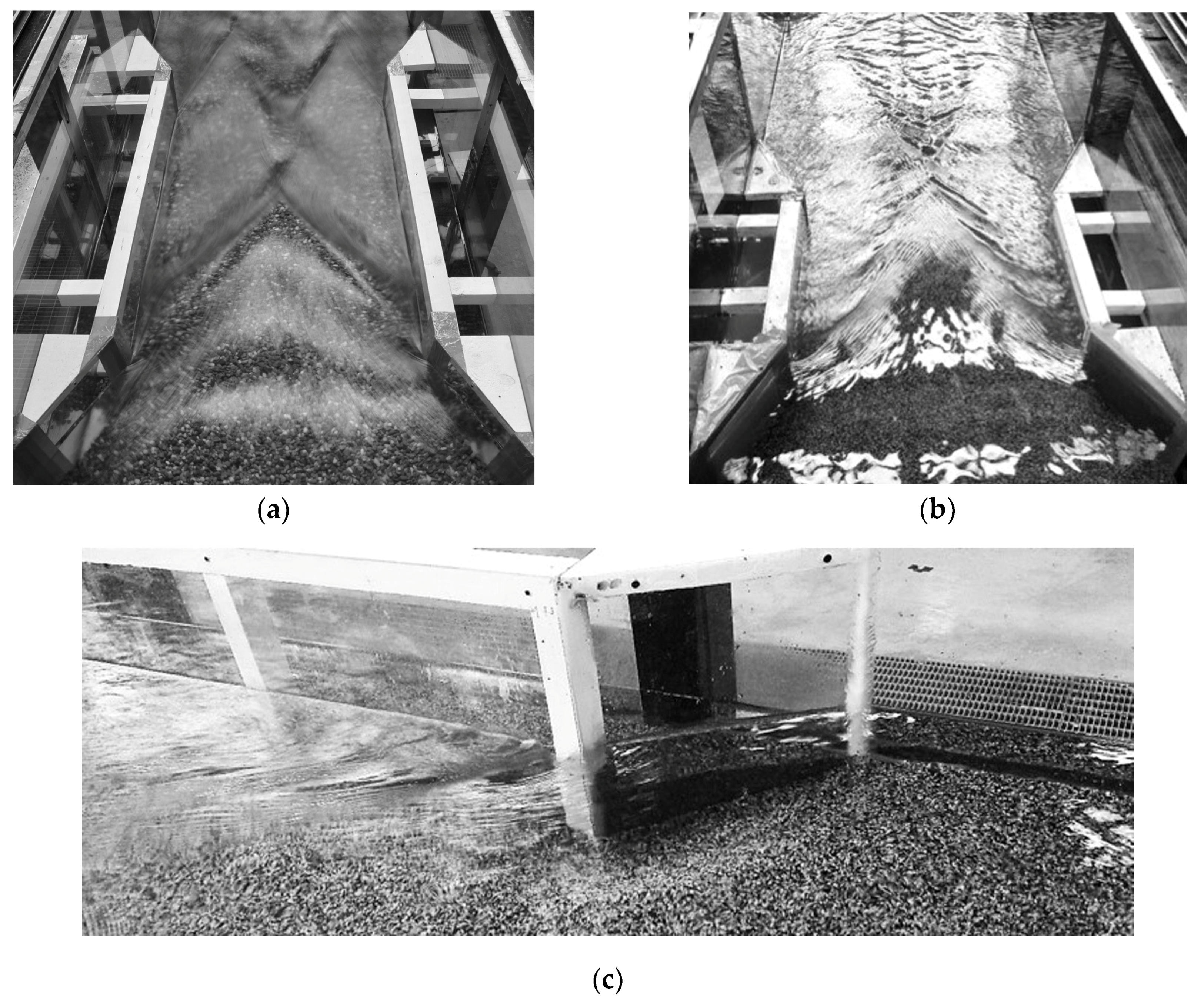
Figure 1a,b show the flow surface at and downstream of the contraction for runs 11 (with l = 1.0 m) and 16 (with l = 0.5 m). In both runs, streamlines converge and interfere almost at the same distance from the inlet upstream end. Hence they diverge by an angle that in case of run 11 is smaller than that of run 16, as a result of the longer extension of the contracted region. It can also be observed that where streamlines diverge, small and very close waves developed for run 16 while more spaced but higher waves for run 11. Finally, Figure 1c shows the free surface and the local scour characteristics at the contraction inlet for run 20. It can be observed the vortex that develops just downstream the edge of the (triangular) inlet element.
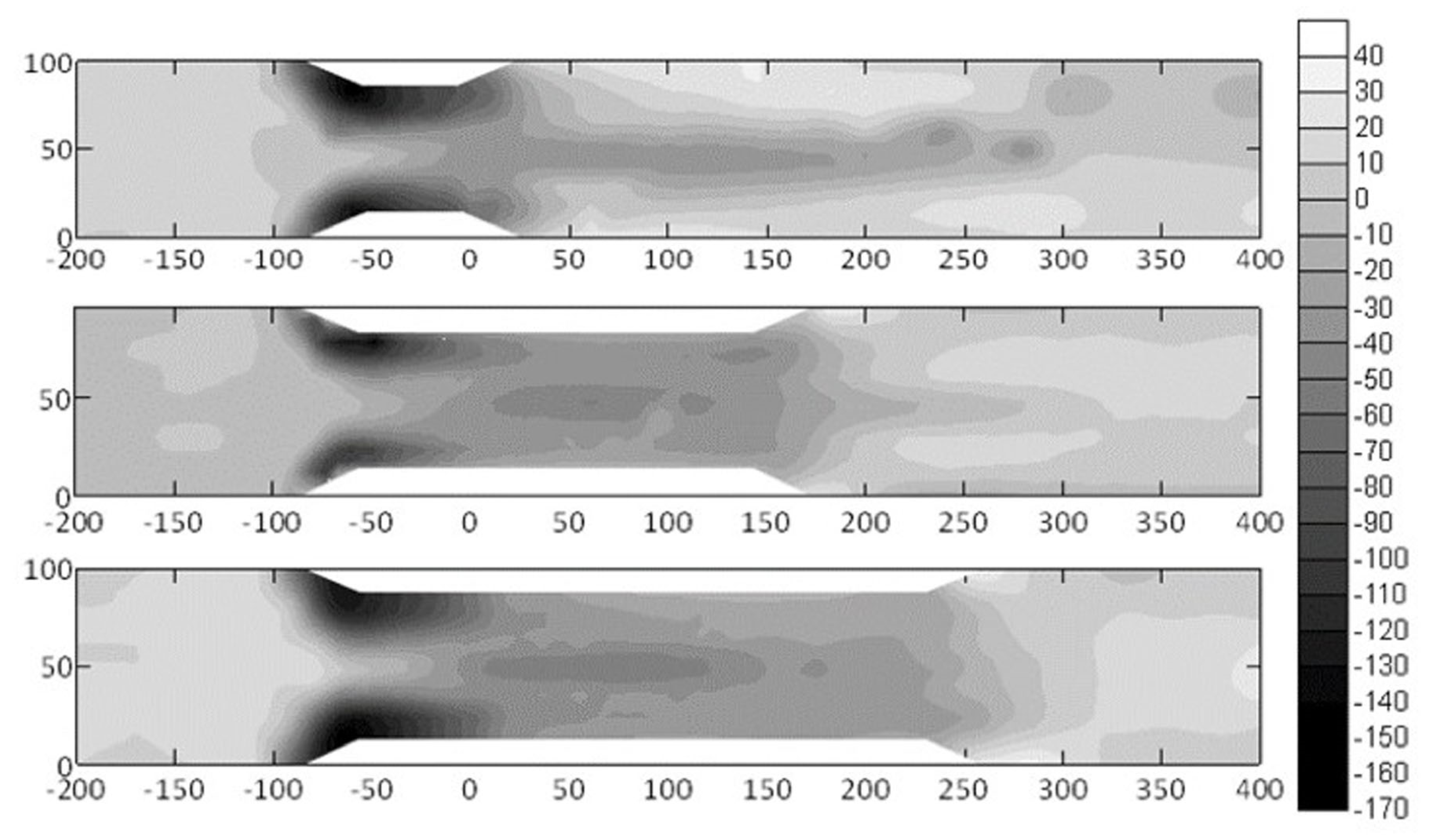
Figure 2 shows the bed morphology at the end of runs 16, 14, and 20 all characterized by the same hydraulic and sediment initial conditions (Q = 0.040 m3/s, h = 0.10 m, d50 = 1.7 mm), and run duration (te = 8 h), but different contraction length l equal to 0.5, 2.0, and 3.0 m, respectively. It is evident that the morphological patterns at the end of the runs were rather different, which emphasizes the need for a deeper understanding of the temporal and spatial morphological changes along and downstream of the contracted reach and that, therefore, beyond the mere knowledge of the maximum scour depth, as in the case of the literature papers. Typically, a single thalweg line develops along the channel centreline. It extends much further downstream of the contracted region in case of the short contraction (run 16), almost eightfold the contraction length and in the middle of two longitudinal bars developed along the channel walls. In case of runs 14 and 20 (long contractions), the extension of the thalweg line is confined to the contracted region. Moreover, experimental observations revealed that the magnitude of scour holes at the contraction inlet appears increasing as the contraction length increases. This effect could be explained by the mutual interaction between local and contraction scour phenomena; bed degradation intensifies as contraction length increases by promoting the progress of scour holes at the contraction inlet.
3. Analysis of Data and Results
The maximum scour depth z* at a given time t can be expressed in functional form as:
z* = f(Vo, ho, ν, ρ, ρs, d50, σ, B, b, l, g, t).
In two-phase flow phenomena with sediment-water interaction, it’s fitting to combine g, ρ, and ρs into g’ = g(ρs − ρ)/ρ [3,25]. Also, the contraction ratio β = b/B can be considered accounting for the joint effect of b and B. Finally, the role of ν in turbulent flow over a rough bed is minor [3]. Therefore, the functional relationship (1) simplifies as:
z* = f(Vo, ho, d50, σ, β, l, g′, t).
By applying the π theorem with repeating variables ho and Vo, and rearranging the parameters likewise Oliveto and Hager [25], one has:
with Fd the densimetric Froude number defined as Vo/(g′d50)1/2 and T a dimensionless time defined as (g′d50)1/2t/ho. The ratio l/B would appear more effective in expressing the relative contraction length. On the other hand, literature studies distinguish between short and long contractions on the basis of l/B. Therefore, by replacing l/ho with l/B and neglecting the effect of ho/B, as it turned out in the regression analysis, Equation (3) can be written as:
The same functional relationship can be applied to L* = l*/ho, in which l* is the scour hole length. The experimental data from the University of Basilicata and those by Gill [6], Webby [2], and Dey and Raikar [3] were considered for regression analysis, which yields the following equation for z*:
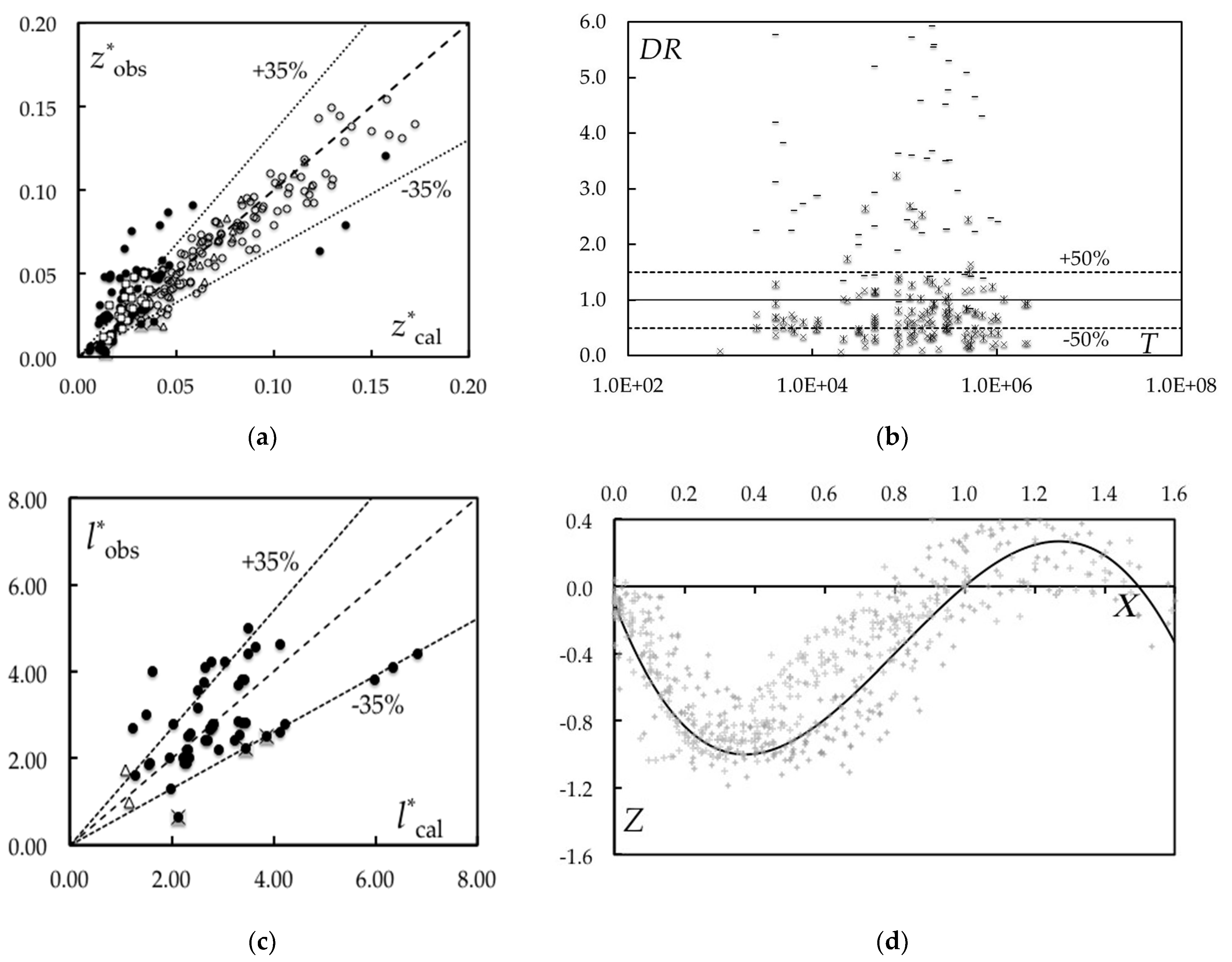
with coefficient of determination r2 = 0.93 between observed and computed values of z* (Figure 3a). T has been conservatively raised to a power 0.10 instead of 0.07, resulting from regression analysis, to better simulate the data collected at University of Basilicata, unaffected by sidewall effects and for which the duration of runs is well defined. Whereas the duration of runs was always taken equal to 24 h for the experimental data by Dey and Raikar [3] (they state that, “The experiments were run under clear-water scour conditions for a period of more than 24 h”), and to 6 h for the experimental data by Gill [6] (he states that, “Each experiment was run for at least 6 h”). Experiments I and II by Webby [2] are clearly documented with the measurement times at final and intermediate stages well defined while for the remaining experiments the duration is not specified and here it was assumed equal to 21 h, close to the durations of the Experiments I and II. Equation (5) is congruent with the boundary conditions according to Z* must be equal to zero when β = 1 and must go to infinity when β goes to zero. It also implies that Z* doesn’t have to be zero for l = 0. Moreover, Z* is a monotonic decreasing function of d50, as expected. In fact, considering that Fd and T depend on d50, Z* scales with 1/d500.59 for given hydraulic conditions. Analogous comments apply to the dependence of Z* on ho. The bed sediments considered in this analysis were almost uniform, therefore the sediment gradation σ is neglected. Equation (5) would provide an acceptable prediction of the scour depth because the observed data lie around the line of perfect agreement with deviations overall within ±35% (Figure 3a). Deviations for small values of z* can be also explained considering that scour depth values were in some cases, though few in number, comparable with the dimension of the grain for runs with gravel. However, the data collected in this study and by Gill [6] appear somewhat underestimated and that would justify the slight increment for the exponent of T in Equation (5), from 0.07 to 0.10, as mentioned above.
Figure 3b shows the performance of well-known literature formulas (i.e., those by Laursen [5], Gill [6], and Lim [7]) in predicting the experimental data collected at University of Basilicata. The discrepancy ratio (DR) is given as a function of the dimensionless time T. DR is the ratio of the predicted value of z* to the observed one. If DR is equal to 1 the estimated value of z* is just the same as the observed one; if DR is larger the predictive model over predicts z*, and if DR is smaller the predictive model would put in under prediction status. The literature formulas here considered refer to the equilibrium condition while the experimental data here analyzed depend on time. Therefore, overall over predictions are expected. In fact, it is what one can deduce from Figure 3b immediately. One might also expect a decreasing trend of DR over T (i.e., for very large values of T equilibrium conditions are much more likely to be attained), but such a trend can be detected only for Laursen’s [5] formula, although weakly. Gill’s [6] formula is likely to cause significant over predictions: the average value of DR was found 6.86 and the standard deviation 10.10. Laursen’s [5] formula was the one that showed the best performance with the average value of DR equal to 1.23, but standard deviation 2.06. Finally, Lim’s [7] formula tends to provide under predictions, though with a reduced dispersion of data. In this case, the average value of DR is equal to 0.58 and the standard deviation 0.35. It remains clear that however the literature formulas under discussion cannot be used in predicting unsteady flow conditions.
Experimental data on l* from literature studies are quite rare. Therefore the experimental data acquired in this study were used for regression analysis and two runs from Webby [2], which yield the following equation:
with r2 = 0.89 between observed and calculated values of l* (Figure 3c). Interestingly, L* was found dependent on l*/B significantly, as expected, but less controlled by the contraction ratio β. As in the case of Equation (5), it is worth noting that L* is a monotonic decreasing function of d50, as expected, and specifically, L* scales with 1/d500.15 for given hydraulic conditions.
Finally, the observed bed profiles along the channel centreline were analysed. After several attempts, an acceptable data scattering was achieved by normalizing the local bed level along the channel centreline with z* and its location from the upstream end of the contraction model with l*. The following equation was found:
where, with reference to the generic local bed level, z, along the channel centreline, Z is the ratio of z to the maximum scour depth z* and X the ratio of the distance of z from the upstream end of the contraction model to l*. The comparison between experimental data and Equation (7) is shown in Figure 3d and it can be noted as data points accumulate around the proposed curve in an agreeable manner. Equation (7) is consistent with the condition that X = 1 for Z = 0, and this condition is not strictly followed by the experimental data because the values of l* are interpolated values. The same reason, applied to z*, explains why Z < 1 for some experimental points. Also, from Equation (7) one can deduce that at X = 0 (i.e., the upstream end of the contraction model) a slight bed lowering of 0.10·z* would occur; z* would locate at x = 0.35 − 0.40·l*; the aggradation region would extend up to 1.50·l*; and its maximum height (around 0.30·|z*|) would locate at x = 1.25 − 1.30·l*.
4. Conclusions
A total of 31 experiments were performed at the University of Basilicata, Italy, to explore the bed morphological changes at and downstream of river contractions. Some experiments were of long duration to assess any conditions of dynamic equilibrium and to allow the development of well-defined bed forms. Some others were of short duration to capture the bed morphology characteristics in the early stages of their temporal evolution.
Experimental observations revealed that typically a thalweg line forms near the channel centerline and extends far beyond the contracted zone especially for short contractions. Moreover, the contraction length would affect the magnitude of the scour hole geometry, and this issue has not received a great deal of attention in the past.
Straightforward equations to predict the temporal development of the longitudinal thalweg profile were suggested in terms of the governing parameters. The main dimensionless parameters controlling the relative thalweg depth are in order of importance: contraction ratio (β), approach densimetric Froude number (Fd), relative submergence (h/d50), relative length of the contracted reach (l/B), and dimensionless time (T). The relative length of the thalweg profile is mainly dependent on l/B, β, and Fd. A new equation for the dimensionless bed profile along the channel centerline was also found. This equation provides additional information on the location of the maximum scour depth and the geometry of the aggradation zone that typically forms just downstream of the scour hole. The ranges of validity for the proposed equations are 18.81 ≤ h/d50 ≤ 117.65, 0.50 ≤ l/B ≤ 3.00, 0.70 ≤ β ≤ 0.90, 1.08 ≤ Fd ≤ 4.02, and 1.0 × 10³ ≤ T ≤ 2.1 × 10⁶ when referring only to the data collected at the University of Basilicata, but they seem all to get wider when considering literature data. Also, some calculations would reveal that local scour depth at the contraction inlet could be confidently estimated by Oliveto and Hager’s [25] formula. Finally, it should be noted that the proposed equations overcome the common distinction between long and short contraction by considering a single approach.
Further research studies might concern the applicability of the proposed time-dependent relationships under unsteady flow regimes, the analysis of bed sediments with density different from that of natural material to check the effective role of the densimetric Froude number, and the investigation of live-bed conditions.
Author Contributions
Conceptualization, G.O.; methodology, G.O. and M.C.M.; software, M.C.M.; validation, G.O. and M.C.M.; formal analysis, G.O.; investigation, G.O. and M.C.M.; resources, G.O. and M.C.M.; data curation, G.O. and M.C.M.; writing—original draft preparation, G.O.; writing—review and editing, G.O. and M.C.M.; supervision, G.O.
Funding
This research received no external funding.
Acknowledgments
The authors wish to thank the technical support from Beniamino Onorati of School of Engineering, University of Basilicata.
Conflicts of Interest
The authors declare no conflict of interest.
References
- Komura, S. Equilibrium depth of scour in long constrictions. J. Hydraul. Div. 1966, 92, 17–37. [Google Scholar]
- Webby, M.G. General scour at a contraction. In 1984 Bridge Design and Research Seminar, Technical Papers, 23 Authors; RRU Bulletin 73; Road Research Unit National Roads Board: Wellington, New Zealand, 1984; pp. 109–118. [Google Scholar]
- Dey, S.; Raikar, R.V. Scour in long contractions. J. Hydraul. Eng. 2005, 131, 1036–1049. [Google Scholar] [CrossRef]
- Straub, L.G. Effect of channel-contraction works upon regime of movable bed-streams. Eos Trans. Am. Geophys. Union 1934, 13, 454–463. [Google Scholar] [CrossRef]
- Laursen, E.M. Scour at bridge crossings. J. Hydraul. Eng. 1960, 86, 39–54. [Google Scholar]
- Gill, M.A. Bed erosion in rectangular long contraction. J. Hydraul. Eng. 1981, 107, 273–284. [Google Scholar]
- Lim, S.Y. Clear water scour in long contractions. Proc. Inst. Civ. Eng. Water Marit. Energy 1993, 101, 93–98. [Google Scholar] [CrossRef]
- Lim, S.Y.; Cheng, N.S. Scouring in long contractions. J. Irrig. Drain. Eng. 1998, 124, 258–261. [Google Scholar] [CrossRef]
- Melville, B.W.; Coleman, S.E. Bridge Scour; Water Resources Publications, LLC: Highlands Ranch, CO, USA, 2000; pp. 173–186. [Google Scholar]
- Briaud, J.L.; Chen, H.C.; Li, Y.; Nurtjahyo, P.; Wang, J. SRICOS-EFA method for contraction scour in fine-grained soils. J. Geotech. Geoenviron. Eng. 2005, 131, 1283–1294. [Google Scholar] [CrossRef]
- Dey, S.; Raikar, R.V. Live-bed scour in long contractions. Int. J. Sediment Res. 2006, 21, 166–170. [Google Scholar]
- Brandimarte, L.; D’Odorico, P.; Montanari, A. A probabilistic approach to the analysis of contraction scour. J. Hydraul. Res. 2006, 44, 654–662. [Google Scholar] [CrossRef]
- Bui, M.D.; Kaveh, K.; Penz, P.; Rutschmann, P. Contraction scour estimation using data-driven methods. J. Appl. Water Eng. Res. 2015, 3, 143–156. [Google Scholar] [CrossRef]
- Raikar, R.V.; Wang, C.Y.; Shih, H.P.; Hong, J.H. Prediction of contraction scour using ANN and GA. Flow Meas. Instrum. 2016, 50, 26–34. [Google Scholar] [CrossRef]
- Najafzadeh, M.; Etemad-Shahidi, A.; Lim, S.Y. Scour prediction in long contractions using ANFIS and SVM. Ocean Eng. 2016, 111, 128–135. [Google Scholar] [CrossRef]
- Benedict, S.T. Clear-Water Abutment and Contraction Scour in the Coastal Plain and Piedmont Provinces of South Carolina, 1996–1999; Water-Resources Investigations Report 03-4064; U.S. Geological Survey: Reston, VA, USA, 2016.
- Mueller, D.S.; Wagner, C.R. Field Observations and Evaluations of Streambed Scour at Bridges; Water Resources Divisions Report No FHWA-RD-03-052; U.S. Geological Survey: Reston, VA, USA, 2005.
- Hong, S.H.; Abid, I. Physical model study of bridge contraction scour. KSCE J. Civ. Eng. 2016, 20, 2578–2585. [Google Scholar] [CrossRef]
- Hayden, J.T.; Puleo, J.A. Near real-time scour monitoring system: Application to Indian River inlet, Delaware. J. Hydraul. Eng. 2011, 137, 1037–1046. [Google Scholar] [CrossRef]
- Li, C.; Zheng, Q. Breakdown of hydrostatic assumption in tidal channel with scour holes. Front. Mar. Sci. 2016, 3, 199. [Google Scholar] [CrossRef]
- Oliveto, G.; Marino, M.C. Experimental and numerical investigation of the bed morphology evolution in river contractions. In Deltas of the Future and What Happens Upstream, Proceedings of the 36th IAHR World Congress, The Hague, The Netherlands, 28 June–3 July 2015; Mynett, A., Ed.; International Association for Hydro-Environment Engineering and Research-IAHR: Madrid, Spain, 2015; pp. 1697–1703. [Google Scholar]
- Oliveto, G.; Marino, M.C. Bed morphology changes at river contractions. In Scour and Erosion, Proceedings of the 8th International Conference on Scour and Erosion, Oxford, UK, 12–15 September 2016; Harris, J., Whitehouse, R., Moxon, S., Eds.; CRC Press, Taylor & Francis Group: London, UK, 2016; pp. 855–860. [Google Scholar]
- Oliveto, G. Sediment transport at river contractions. WIT Trans. Ecol. Environ. 2019, 234, 1–7. [Google Scholar] [CrossRef]
- Graf, W.H.; Altinakar, M.S. Fluvial Hydraulics-Flow and Transport Processes in Channels of Simple Geometry; John Wiley & Sons Inc.: Chichester, UK, 1998; pp. 10–12. [Google Scholar]
- Oliveto, G.; Hager, W.H. Temporal evolution of clear-water pier and abutment scour. J. Hydraul. Eng. 2002, 128, 811–820. [Google Scholar] [CrossRef]
- Hager, W.H.; Oliveto, G. Shields’ entrainment criterion in bridge hydraulics. J. Hydraul. Eng. 2002, 128, 538–542. [Google Scholar] [CrossRef]
Figure 1.
Free surface characteristics for runs 11 (a) and 16 (b). Flow streamlines and local scour at the contraction inlet for run 20 (c).
Figure 1.
Free surface characteristics for runs 11 (a) and 16 (b). Flow streamlines and local scour at the contraction inlet for run 20 (c).

Figure 2.
Comparison of bed morphologies observed at the end of runs 16 (map at the top), 14 (map in the middle), and 20 (map at the bottom). All the runs lasted 8 h and were characterized by the same approach flow conditions and mobile bed, but different contraction length equal to 0.5, 2.00, and 3.00 m, respectively. Axis coordinates are in cm while measurements in mm.

Figure 3.
(a) Comparison between observed (subscript “obs”) and calculated (“cal”) values of z* for the data collected at the University of Basilicata (●) with cross symbol indicating gravel and the data by: Gill [6] (☐), Webby [2] (△), and Dey and Raikar [3] (O). The values of z* are in meters; (b) discrepancy ratio (DR) as a function of the dimensionless time T for Laursen’s [5] (🞶), Gill’s [6] (✕), and Lim’s [7] (–) formulas; (c) comparison between observed and calculated values of l* for the data collected at the University of Basilicata (●) with cross symbol indicating gravel and by Webby [2] (△). The values of l* are in meters; (d) comparison between observed axial bed profiles (+) and Equation (7) (full curve).


Table 1.
Test conditions and peculiar characteristics of the bed morphology.
| Run | λ (-) | β (-) | Ro·10−5 (-) | Fo (-) | Fd (-) | Fdi (-) | T (h) | z* (m) | l* (m) |
|---|---|---|---|---|---|---|---|---|---|
| #1 | 1.00 | 0.90 | 1.16 | 0.37 | 2.29 | 3.24 | 89.5 | 0.0049 | 2.850 |
| 157.5 | 0.0059 | 3.800 | |||||||
| 209.5 | 0.0072 | 3.800 | |||||||
| 353.5 | 0.0079 | 4.400 | |||||||
| 380.0 | 0.0078 | 5.000 | |||||||
| #2 | 1.00 | 0.90 | 0.67 | 0.46 | 2.13 | 2.99 | 24.0 | 0.0035 | 2.800 |
| 47.0 | 0.0050 | - | |||||||
| 99.3 | 0.0060 | - | |||||||
| #3 | 1.00 | 0.90 | 1.62 | 0.33 | 2.40 | 3.39 | 20.5 | 0.0032 | 2.600 |
| 38.9 | 0.0041 | 2.800 | |||||||
| #4 | 1.00 | 0.80 | 1.20 | 0.39 | 2.38 | 3.23 | 8.5 | 0.0140 | 2.580 |
| 36.0 | 0.0172 | 3.150 | |||||||
| 101.0 | 0.0206 | 3.750 | |||||||
| 121.8 | 0.0222 | 4.100 | |||||||
| #5 | 1.00 | 0.80 | 0.72 | 0.45 | 2.17 | 3.01 | 13.6 | 0.0222 | - |
| 92.8 | 0.0236 | - | |||||||
| 110.9 | 0.0243 | - | |||||||
| #6 | 1.00 | 0.80 | 1.64 | 0.33 | 2.44 | 3.39 | 28.7 | 0.0220 | 2.420 |
| 52.6 | 0.0245 | 2.550 | |||||||
| 76.3 | 0.0259 | 2.830 | |||||||
| 117.8 | 0.0269 | 2.830 | |||||||
| #7 | 1.00 | 0.70 | 1.17 | 0.40 | 2.40 | 3.21 | 1.9 | 0.0400 | - |
| 18.1 | 0.0471 | - | |||||||
| 26.1 | 0.0522 | - | |||||||
| 47.3 | 0.0507 | - | |||||||
| 97.9 | 0.0516 | - | |||||||
| #8 | 1.00 | 0.70 | 0.63 | 0.43 | 2.01 | 2.98 | 0.3 | 0.0306 | - |
| 3.7 | 0.0477 | - | |||||||
| 45.2 | 0.0473 | - | |||||||
| 52.8 | 0.0482 | - | |||||||
| 71.5 | 0.0494 | - | |||||||
| #9 | 1.00 | 0.70 | 1.62 | 0.33 | 2.41 | 3.39 | 1.0 | 0.0409 | 2.000 |
| 21.3 | 0.0473 | 2.430 | |||||||
| 30.1 | 0.0477 | 2.430 | |||||||
| 43.8 | 0.0484 | 2.680 | |||||||
| 49.8 | 0.0466 | 2.700 | |||||||
| 69.6 | 0.0490 | 2.720 | |||||||
| 76.6 | 0.0490 | 2.800 | |||||||
| 94.6 | 0.0579 | 2.800 | |||||||
| #10 | 1.00 | 0.70 | 0.31 | 1.82 | 3.21 | 0.2 | 0.0032 | 1.600 | |
| 0.88 | 18.8 | 0.0094 | 1.850 | ||||||
| 21.3 | 0.0108 | 1.900 | |||||||
| #11 (+) | 1.00 | 0.70 | 1.83 | 0.32 | 1.08 | 3.00 | 2.5 | 0.0027 | 0.640 |
| #12 (+) | 1.00 | 0.70 | 3.00 | 0.42 | 1.55 | 3.06 | 5.5 | 0.0196 | 2.230 |
| 72.0 | 0.0212 | 2.500 | |||||||
| #13 | 2.00 | 0.70 | 1.62 | 0.33 | 2.41 | 3.39 | 8.0 | 0.0863 | 3.680 |
| #14 | 2.00 | 0.70 | 1.17 | 0.40 | 2.41 | 3.21 | 8.0 | 0.0492 | 3.560 |
| #15 | 2.00 | 0.70 | 0.88 | 0.31 | 1.82 | 3.21 | 48.0 | 0.0501 | - |
| #16 | 0.50 | 0.70 | 1.17 | 0.40 | 2.41 | 3.21 | 8.0 | 0.0390 | 4.000 |
| #17 | 0.50 | 0.70 | 1.62 | 0.33 | 2.41 | 3.39 | 1.0 | 0.0298 | 2.000 |
| 21.3 | 0.0280 | 2.000 | |||||||
| 30.1 | 0.0300 | 1.900 | |||||||
| 43.8 | 0.0280 | 1.900 | |||||||
| 49.8 | 0.0290 | 2.200 | |||||||
| 69.6 | 0.0380 | 2.200 | |||||||
| #18 | 0.50 | 0.70 | 0.88 | 0.30 | 1.81 | 3.21 | 8.0 | 0.0220 | 2.700 |
| 25.0 | 0.0250 | - | |||||||
| 50.0 | 0.0240 | - | |||||||
| #19 | 0.50 | 0.70 | 1.50 | 0.21 | 1.81 | 3.51 | 8.0 | 0.0294 | 1.300 |
| #20 | 3.00 | 0.70 | 1.17 | 0.40 | 2.41 | 3.21 | 8.0 | 0.0790 | 4.230 |
| #21 | 3.00 | 0.70 | 1.17 | 0.40 | 2.41 | 3.21 | 1.0 | 0.0510 | 4.230 |
| #22 | 3.00 | 0.70 | 1.62 | 0.33 | 2.41 | 3.39 | 1.0 | 0.0550 | 4.561 |
| 21.0 | 0.0910 | 4.614 | |||||||
| #23 | 3.00 | 0.70 | 0.63 | 0.50 | 2.19 | 2.95 | 2.0 | 0.0470 | - |
| #24 | 3.00 | 0.70 | 0.63 | 0.50 | 2.19 | 2.95 | 8.0 | 0.0650 | - |
| #25 | 3.00 | 0.70 | 0.63 | 0.50 | 2.19 | 2.95 | 48.0 | 0.0750 | - |
| #26 | 3.00 | 0.70 | 2.70 | 0.55 | 4.02 | 3.39 | 2.0 | 0.0630 | 3.800 |
| #27 | 3.00 | 0.70 | 2.70 | 0.55 | 4.02 | 3.39 | 8.0 | 0.0790 | 4.100 |
| #28 | 3.00 | 0.70 | 2.70 | 0.55 | 4.02 | 3.39 | 48.0 | 0.1205 | 4.400 |
| #29 | 1.00 | 0.80 | 1.29 | 0.39 | 2.47 | 3.25 | 1.2 | 0.0386 | 2.500 |
| #30 | 1.00 | 0.80 | 0.75 | 0.48 | 2.30 | 3.01 | 1.2 | 0.0200 | 3.000 |
| #31 | 1.00 | 0.80 | 1.69 | 0.36 | 2.60 | 3.37 | 1.2 | 0.0344 | 2.200 |
(+) Runs with mobile bed in gravel.
© 2019 by the authors. Licensee MDPI, Basel, Switzerland. This article is an open access article distributed under the terms and conditions of the Creative Commons Attribution (CC BY) license (http://creativecommons.org/licenses/by/4.0/).
Share and Cite
MDPI and ACS Style
Oliveto, G.; Marino, M.C. Morphological Patterns at River Contractions. Water 2019, 11, 1683. https://doi.org/10.3390/w11081683
AMA Style
Oliveto G, Marino MC. Morphological Patterns at River Contractions. Water. 2019; 11(8):1683. https://doi.org/10.3390/w11081683
Chicago/Turabian StyleOliveto, Giuseppe, and Maria Cristina Marino. 2019. "Morphological Patterns at River Contractions" Water 11, no. 8: 1683. https://doi.org/10.3390/w11081683
Note that from the first issue of 2016, this journal uses article numbers instead of page numbers. See further details here.