IPEAT+: A Built-In Optimization and Automatic Calibration Tool of SWAT+

Abstract

For almost 30 years, the Soil and Water Assessment Tool (SWAT) has been successfully implemented to address issues around various scientific subjects in the world. On the other hand, it has been reaching to the limit of potential flexibility in further development by the current structure. The new generation SWAT, dubbed SWAT+, was released recently with entirely new coding features. SWAT+ is designed to have far more advanced functions and capacities to handle challenging watershed modeling tasks for hydrologic and water quality processes. However, it is still inevitable to conduct model calibration before the SWAT+ model is applied to engineering projects and research programs. The primary goal of this study is to develop an open-source, easy-to-operate automatic calibration tool for SWAT+, dubbed IPEAT+ (Integrated Parameter Estimation and Uncertainty Analysis Tool Plus). There are four major advantages: (i) Open-source code to general users; (ii) compiled and integrated directly with SWAT+ source code as a single executable; (iii) supported by the SWAT developer group; and, (iv) built with efficient optimization technique. The coupling work between IPEAT+ and SWAT+ is fairly simple, which can be conducted by users with minor efforts. IPEAT+ will be regularly updated with the latest SWAT+ revision. If users would like to integrate IPEAT+ with various versions of SWAT+, only few lines in the SWAT+ source code are required to be updated. IPEAT+ is the first automatic calibration tool integrated with SWAT+ source code. Users can take advantage of the tool to pursue more cutting-edge and forward-thinking scientific questions.

1. Introduction

To better represent hydrologic and nutrient processes in natural systems, watershed simulation models such as the Soil and Water Assessment Tool (SWAT) [1], WetQual [2], Agricultural Policy/Environmental eXtender (APEX) [3], and Hydrological Simulation Program-Fortran (HSPF) [4], have been intensively developed and implemented in various scientific projects in the past 30 years. Among the commonly adopted models, the SWAT model is one of the most popular platforms which generated thousands of peer-reviewed publications in academic community (SWAT Literature Database for Peer-Reviewed Articles; https://www.card.iastate.edu/swat_articles/INDEX.ASPX). In addition to educational contributions, SWAT is also used by government policy makers such as the Conservation Effects Assessment Project conducted in the United States (CEAP) [5,6,7].

SWAT is used to perform watershed-scale simulations for flow, sediment, nutrient, pesticide, and bacteria [8,9,10,11,12]. Before one can apply SWAT for actual practices such as assigning conservation scenarios or investigating climate change impacts, the corresponding model parameters should be properly adjusted in model calibration processes to reflect watershed systems [13,14,15,16,17]. However, a complex watershed simulation model like SWAT comes along with a large number of undefined model parameters, whereas the ordinary manual calibration approach may not well serve some projects in a timely matter (note that manual calibration approach is so far the best way for modelers to understand detailed model processes). Fortunately, programs and software are available for users to carry through calibration routines such as SWAT-CUP [18] and IPEAT (Integrated Parameter Estimation and Uncertainty Analysis Tool) [19]. Users can take advantage of such tools to conduct model calibration by optional parameter searching algorithms.

After almost 30 years development, proficiency of the SWAT model has reached to the limit where potential flexibility is restricted by the current structure. Therefore, a new generation SWAT, dubbed SWAT+, has recently been release with entirely new coding features [20]. SWAT+ is a lot more flexible in terms of spatial representation and the associated modular codes were designed to facilitate future applications and development for general users. One of the new features is that users may conduct manual calibration in easier ways via the calibration.cal file, whereas users can define parameter values in basin, subbasin, and HRU (Hydrologic Response Unit) levels. However, one may need automatic calibration tool(s) once the required calibration load is significant. For example, manual calibration is: (i) More time consuming in altering parameters one by one; (ii) highly dependent on users’ experience in both hydrologic or water quality processes; and, (iii) users must be very familiar with the structure or organization of a model (e.g., groundwater parameters).

IPEAT was developed to perform automatic calibration with the SWAT model [19]. The overall goal of IPEAT is to provide a computational framework that can be applied to other models, such as APEX-CUTE [21]. The main advantage of IPEAT is that users could flexibly add additional functions based on their needs since the source code is open to the public, unlike other calibration tools. For example, uses can assign soft data constraints to address interior watershed processes during model simulations (non-temporal data such as denitrification rate, [22]). In addition, the corresponding optimization algorithm can also be replaced with minor efforts. On the other hand, the hitch of IPEAT is that it’s currently a MATLAB-based program. Therefore, users are required to have MATLAB installed on their operation systems.

As it was mentioned earlier, there are some automatic calibration tools available for the SWAT model. However, some users still feel the need of developing their own tools because of the conceivable limitations (e.g., not open source, required software to operate, or difficult to upgrade for advanced explorations). Therefore, much unnecessary time was spent on research for the tedious computer programming skills and operations research. Until now, no automatic calibration tool is available for SWAT+. It is necessary to have this issue resolved while the new generation SWAT (SWAT+) is officially released.

The goal of this research is to develop an open-source, easy-to-operate automatic calibration tool (IPEAT+) for SWAT+. Specifically, IPEAT+ offers the following five advantages: (i) IPEAT+ is an open-source program so that users can modify or customize it freely; (ii) IPEAT+ is compiled directly with SWAT+ under the FORTRAN coding environment and can be executed without installing any additional program; (iii) IPEAT+ is supported by the SWAT developers group and the corresponding technical support is available; and, (iv) IPEAT+ is using a fast optimization algorithm (which can also be replaced by other algorithms with minor efforts) to ensure computational efficiency during calibration.

In this study, the SWAT+ model was used to conduct watershed simulation at the Middle Bosque River Watershed (MBRW) in the State of Texas, USA. Nine parameters were calibrated and validated for hydrologic processes and corresponding comparisons by implementing statistical measures, behavior definition, and uncertainty analysis.

2. Materials and Methods

2.1. The SWAT/SWAT+ Model

2.1.1. SWAT

The SWAT model was developed in the early 1990s by the United States Department of Agriculture—Agricultural Research Service (USDA-ARS) to address the fate of pollutants caused by anthropogenic activities, especially nonpoint sources pollution (NPS) [1]. The early version of SWAT was the combination of coupling ROTO [23] and SWRRB [24] models. It is a continuous-time, process-based, spatially distributed model that has been used to perform wide variety of watershed-scale applications by providing scientifically credible solutions. Hydrologic (surface and subsurface flows), sediment, and nutrient/pesticide processes with changing management practices can be reasonably simulated by large amount of governing functions. The special feature of SWAT is the use of HRUs where designated land use, soil type, and slope information can be grouped into files for each subbasin. Outputs at the HRU level are aggregated at subbasin level, and eventually delivered from upstream to downstream subbasin via channel routing. This approach is fairly useful back in the time when computational speed was still quite slow. On the other hand, users can assign one HRU per each subbasin so that the SWAT project will be closer to a physically-based model (instead of semi-physically-based) with given modern computer technology. SWAT has been applied globally on various subjects such as Great Lakes in the United States [25,26,27], Blue Nile Basin in Africa [28], and Yellow River Basin in China. More than 3,000 peer-reviewed articles are available as references for users in the official database of SWAT community [29].

2.1.2. SWAT+

SWAT+ is the new generation SWAT model developed to be more flexible in advanced upgrades and expansion. The primary contribution of SWAT+ is that the model has been reconstructed as independent modules (objects) so that it’s a lot easier in terms of model maintenance and the corresponding development as well. In addition to modularization, there are also some key developments to enhance the performance of the model. For example, new functionalities of aquifers and reservoir operation rules are available in SWAT+. Aquifers are used to be controlled exclusively in HRUs. Now the corresponding aquifer boundaries can be defined flexibly without following the limitations by HRUs. As for reservoir functions, it was one of the primary setbacks of the SWAT model. Reservoir releases may play significant role in watershed responses especially for those with relatively larger ones. Users now can assign detailed operation rules effortlessly in SWAT+ so that reservoir simulation outputs can be a lot closer to actual operation routines. Primary differences between SWAT+ and SWAT models are shown in

Table 1. Primary differences of functionalities between SWAT and SWAT+.

Category	SWAT+	SWAT
Calibration Support	Users can manually calibrate SWAT+ by using calibration.cal	Not Supported
Reservoir Operation	Users can assign operation rules	Not Supported
Coding Flexibility	Easy to modify/upgrade modularized coding structure	Conventional
Aquifer Boundary	Can be defined flexibly without limitations	Used to be linked with HRUs*
Connectivity	Users can define individual watershed objects	Limited spatial flexibility

HRUs*: Hydrologic Response Units.

.

There are others spatial modules with designate functions: (i) outlets, can be used to add/remove water from the watershed; (ii) canals; can be used to conduct water diversion among irrigation regions; (iii) pumps, can be extracted from any aquifer to specified spatial object; (iv) herds, can be applied to biomass and the associated grazing conditions; and, (v) water rights, can be assigned by different share of water demand. More details can also be found in [17].

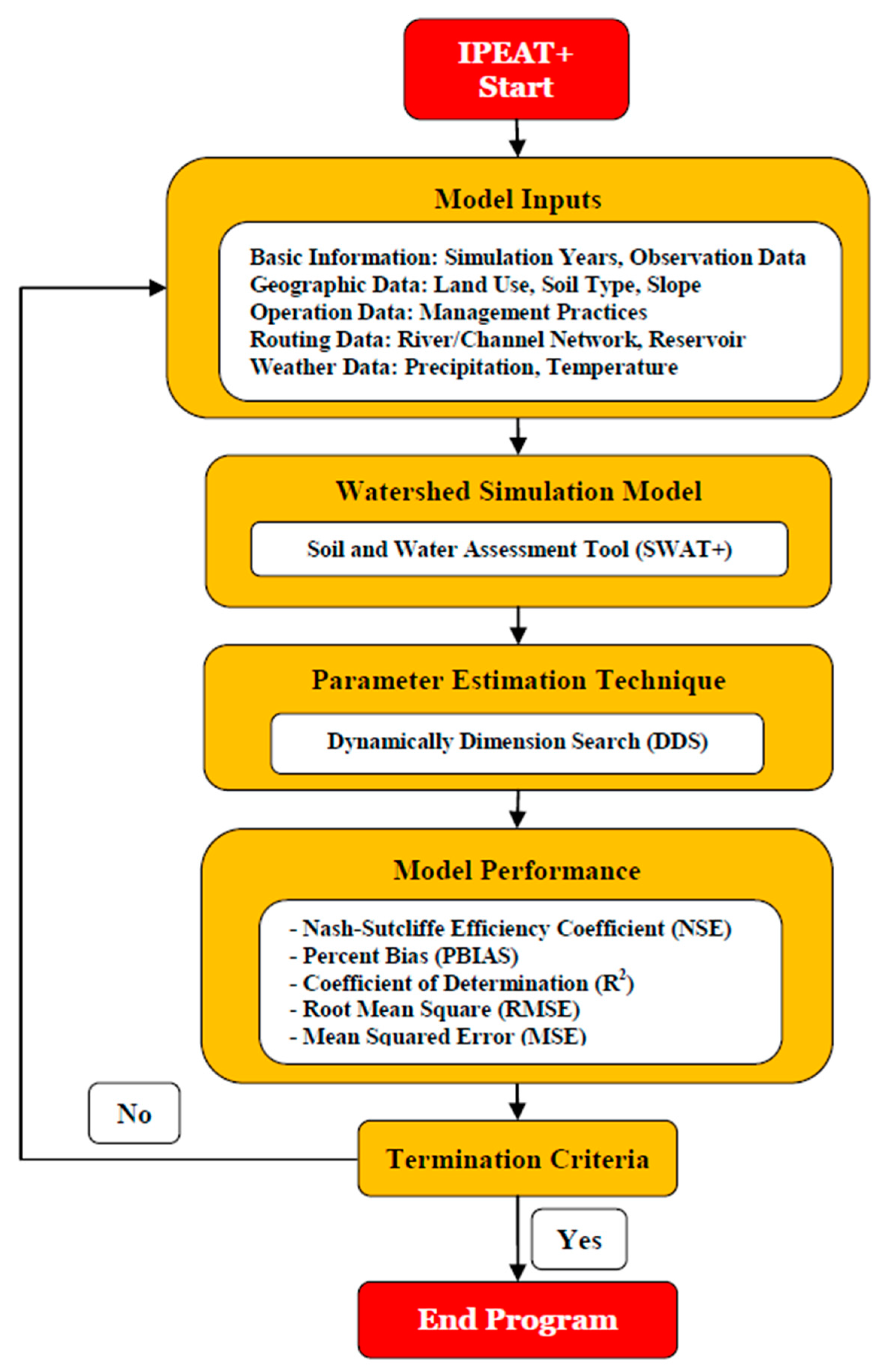
2.2. IPEAT/IPEAT+ Framework

Some commonly adopted SWAT automatic calibration programs are not open-source to the public. It is difficult or sometimes impossible to explore more advanced subjects (e.g., incorporation of non-temporal-based soft data within interior watershed processes, [22]) without changing the program accordingly. IPEAT is a computational framework that was developed to not only conduct automatic calibration but also investigate uncertainty from multiple sources such as model parameters, system structure, forcing inputs, and measurement outputs [19]. IPEAT was initially linked with SWAT under the MATLAB environment whereas users have to install the corresponding program to execute all functions. In IPEAT, the Dynamically Dimension Search (DDS) was selected to be the default parameter searching engine. It has been shown that DDS outperformed mainstream optimization techniques with superior performance in terms of computational speed and the ability to break through local solutions [30].

The same framework was also implemented to other model such as APEX (referred as APEX-CUTE, available in both MATLAB and Python programs) which is the version that incorporates IPEAT framework [21]. It is a field-scale watershed simulation program maintained by the Texas A&M University and the U.S. Department of Agriculture. Applications of IPEAT can be found in literature which is off the focus of this manuscript.

The primary pitfall of IPEAT with SWAT is that it is still a MATLAB-based platform. One needs to prepare/purchase MATLAB package to execute the program, which could potentially be a hindrance to some international users. In addition, similar to other automatic calibration programs, MATLAB is serving the purpose of data management routines before and after SWAT (or other models as well) execution. Specifically, open & read targeted files; write & save updated information (e.g., new parameter values) into targeted files; calculation of error statistics; print desired (organized) modeling outputs; and, preparation of next runs(s) or proceed termination criteria. However, thousands of simulations may be conducted for calibration purposes in a general SWAT project so the projected computational speed could be prolonged due to the communication between FORTRAN executable and MATLAB-based IPEAT program. Therefore, IPEAT+ is developed in FORTRAN and linked with SWAT+ directly in the source code to save communication time between programs and users do not need to install any additional programs anymore.

As shown in Figure 1, the computational structure of IPEAT+ can be categorized into five parts: (i) Model initialization; (ii) model simulation; (iii) execution of parameter estimation technique; (iv) calculation of statistics; and, (v) implementation of termination criteria. The calculation routines are similar to most available calibration approaches. On the other hand, some detailed controlling setups are described in the following sections.

2.3. IPEAT+ Control Panel and Settings

There are three primary control files to conduct automatic calibration: (i) Technical Control File [IPEAT_Control.set]; (ii) Parameter Setting File [IPEAT_Para.set]; and, (iii) Observation File(s) [IPEAT_ObsXY.set]. Detailed description is as follows.

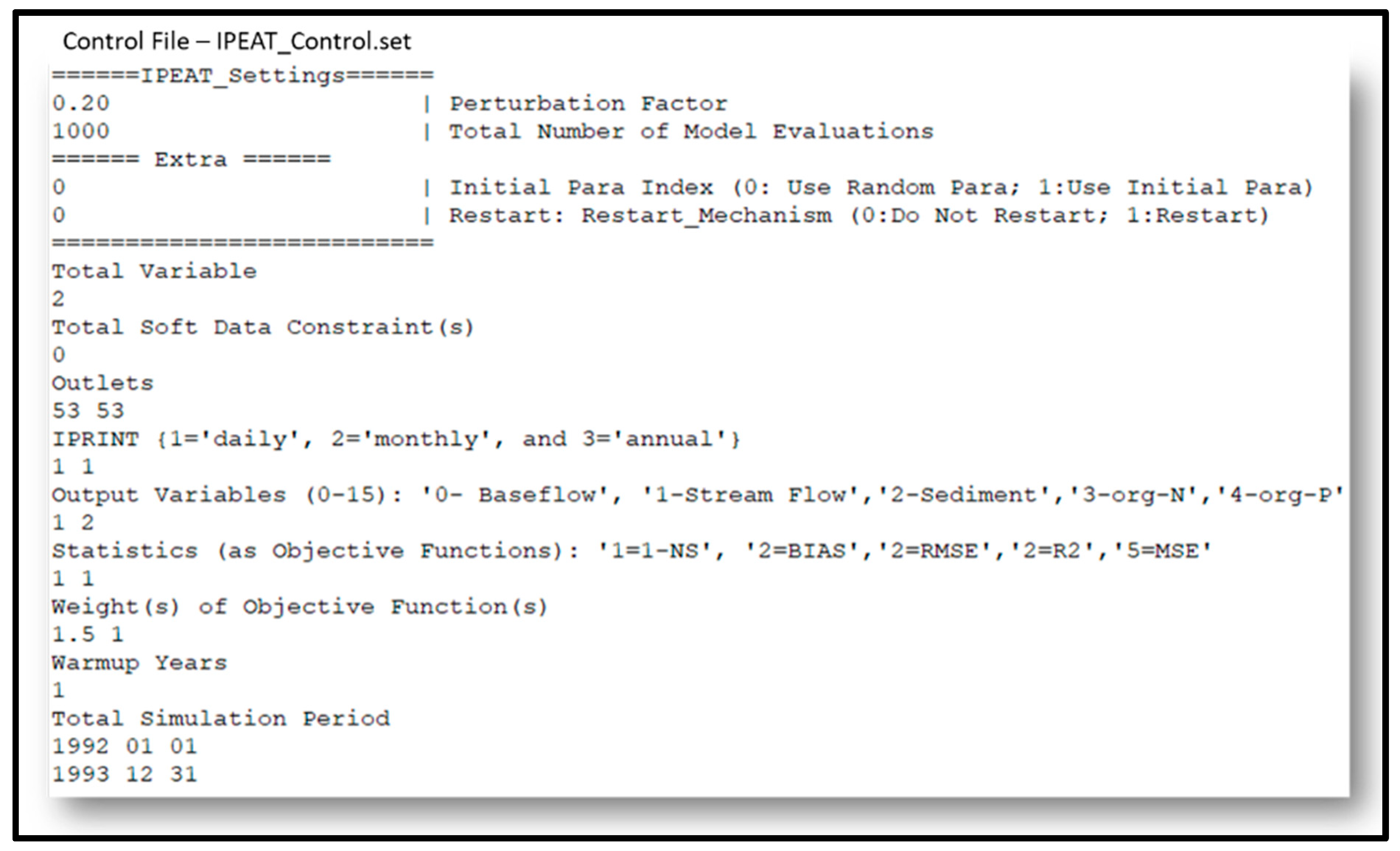
2.3.1. Technical Control File

IPEAT_Control.set is the most important control file in IPEAT+ operation. As shown in Figure 2, users shall define many simulation details here. The first part of the control file is to define variables in conducting optimization algorithm: (i) Perturbation Factor (PF): The default value of PF is 0.2, which has been validated in literature and users do not need to adjust this value to find better solutions [31]; (ii) Total Number of Model Evaluation (TotalRuns): The maximum simulation runs defined before conducting calibration routines; (iii) Initial Para Index (InitialParaIndex): Users can start automatic calibration from randomly selected initial parameter set (InitialParaIndex = 0), or, it is also supported to begin with designated one (InitialParaIndex = 1); and, (iv) Restart Mechanism (RestartIndex): Users can choose to start from the 1st run (RestartIndex = 0), or, restart model simulation from the breaking run while terminated in case simulations are unfortunate incidents (RestartIndex = 1).

The second part of the control file is to define calibration variables. There are nine major components: (i) Total Variable: The number of output variables that users are trying to calibrate; (ii) Total Soft Data Constraint(s): The number of soft data constraints that users are trying to incorporate during automatic calibration; (iii) Outlets: Designated number of outlet(s) that users are going to calibrate; (iv) IPRINT: Simulation time period that users intend to calibrate; (v) Output Variables: Desired output variables during calibration (units for streamflow, sediment and nutrient loads are m³/sec, ton/day, and kg/day): (vi) Statistics (as Objective Functions): Predefined objective function(s) during calibration; (vii) Weight(s) of Objective Function(s): Users can define the corresponding weight for each objective function to highlight the importance of individual variable; (viii) Warmup Years: Additional model simulation years before designated calibration time period; and, (ix) Total Simulation Period: Total simulation time for model simulations. The given example in Figure 2 demonstrated that two variables are defined for automatic calibration with no soft data constraint involved. The first variable is defined at outlet 53, in daily time step for streamflow rate (m³/sec) and the corresponding objective function is 1-NS (Nash-Sutcliffe Efficiency Coefficient) [32] with the given weight of 1.5. The second variable represents at outlet 54, in daily time step for sediment load (ton/day) and the corresponding objective function is 1-NS (Nash-Sutcliffe Efficiency Coefficient) with the given weight of 1.0.

One can find that calibration details of different variables are defined by order in each row from (iii) through (vii). Users can take the same concept for higher dimensional scenarios. Please note that it’s not recommended to mix different objective functions (e.g., mixing 1-NS with PBIAS in the same calibration scenario) since that may show no statistical sense in the derived results.

2.3.2. Parameter Setting File

In SWAT, calibration of model parameters can be tedious even by taking the automatic approaches because users have to adjust parameter values in thousands (or more) of SWAT input files for the whole watershed project. Fortunately in SWAT+, users can conduct manual calibration by changing parameter values in the calibration.cal file with a lot less effort. In IPEAT+, IPEAT_Para.set is used to define required information of the most important calibration parameters. The format of IPEAT_Para.set is following the same pattern of cal_parms.cal which contains the full list candidate parameters available for calibration in SWAT+. As shown in Figure 3a, three columns are added for users to select candidate parameters and to define initial values if desired. Specifically, InitialValue is designated initial parameter value if users have preference. CHG_TYPE (1 = abs; 2 = %) is the index that users can calibrate parameters by in scales of absolute values or percentage. Selection (1 = Selected; 0 = NotSelected) is the index that users should use this index to decide which parameters are included in calibration).

2.3.3. Observation Data File(s)

The naming format of observation file is IPEAT_ObsXY.set, whereas X represents time steps and Y is the corresponding outlet number. For example, IPEAT_ObsDay53.set denotes daily observation at outlet 53. The general format of observation file is shown in Figure 3b. The first three columns are time identifiers for year, month, and day. The following columns are streamflow (sf(m³/s)), sediment (sed(t/ha)) load, and nutrient loads (organic nitrogen: orgn(kg/ha), organic phosphorus: orgp(kg/ha), nitrate: NO₃⁻-N (kg/ha), ammonia: NH₄⁺-N (kg/ha), nitrite: NO₂-N (kg/ha), mineral phosphorus: minp(kg/ha), soluble pesticide: solpst(mg/ha), pesticide in sorption: sorpst(mg/ha), total phosphorus: tp(kg/ha), total nitrogen: tn(kg/ha), and total pesticide: tpst(ppb)). For calibration purpose, users can assign the value of “−99” for missing data and the optimization routines will skip those time steps while calculating statistics.

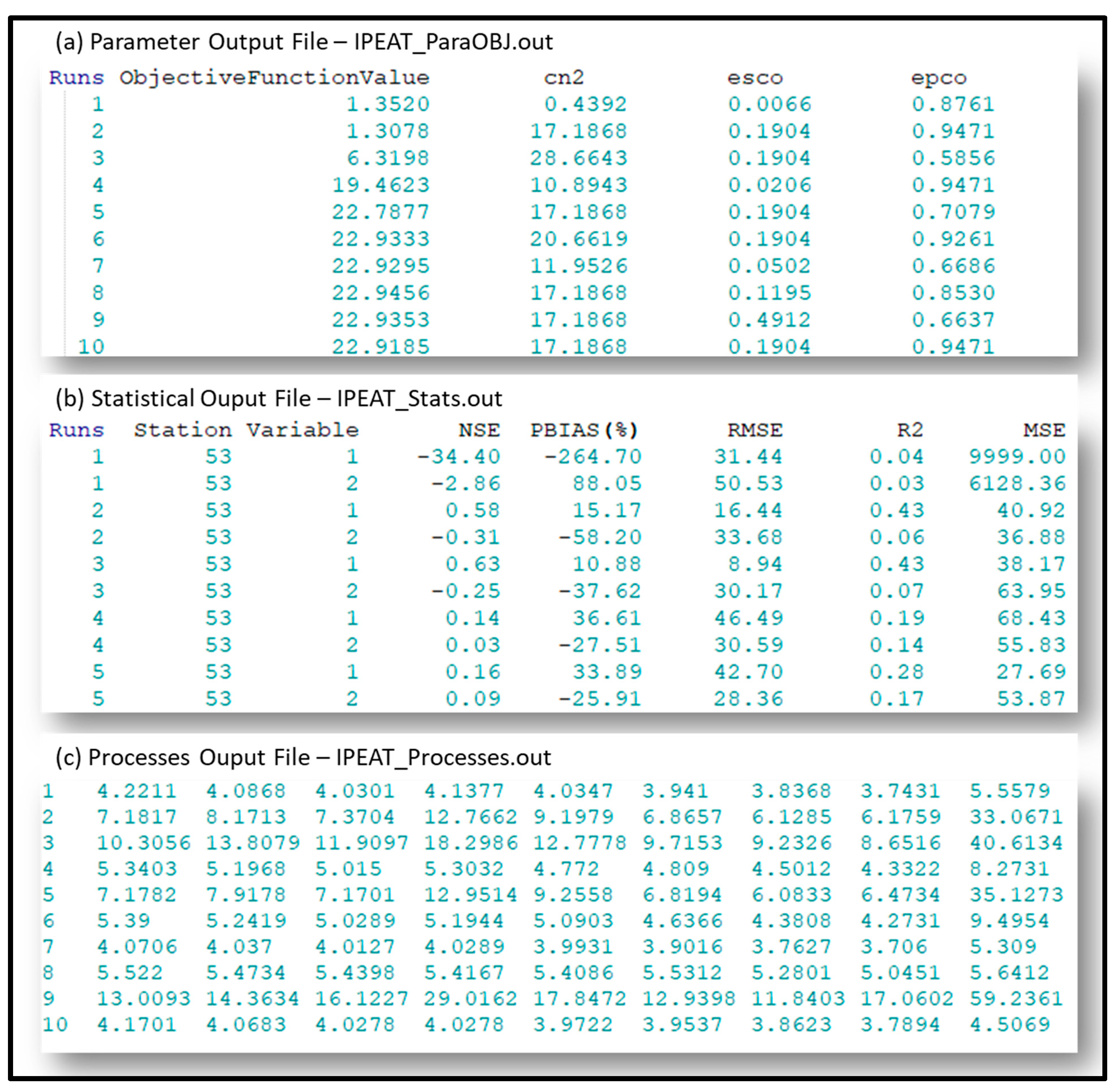
2.4. IPEAT+ Output Files

There are two primary output files in IPEAT+ associated with automatic calibration: (i) IPEAT_ParaOBJ.out: To store calibration outputs for parameter sets and the corresponding objective function values; and, (ii) IPEAT_Stats.out: Statistics (NSE: Nash-Sutcliffe Efficiency Coefficient; PBIAS: Percent Bias; RMSE: Root Mean Square Error; R²: Coefficient of Determination; and, MSE: Mean Squared Error) of individual outlet station in each run are stored in this file. Detailed description of output files is as follows.

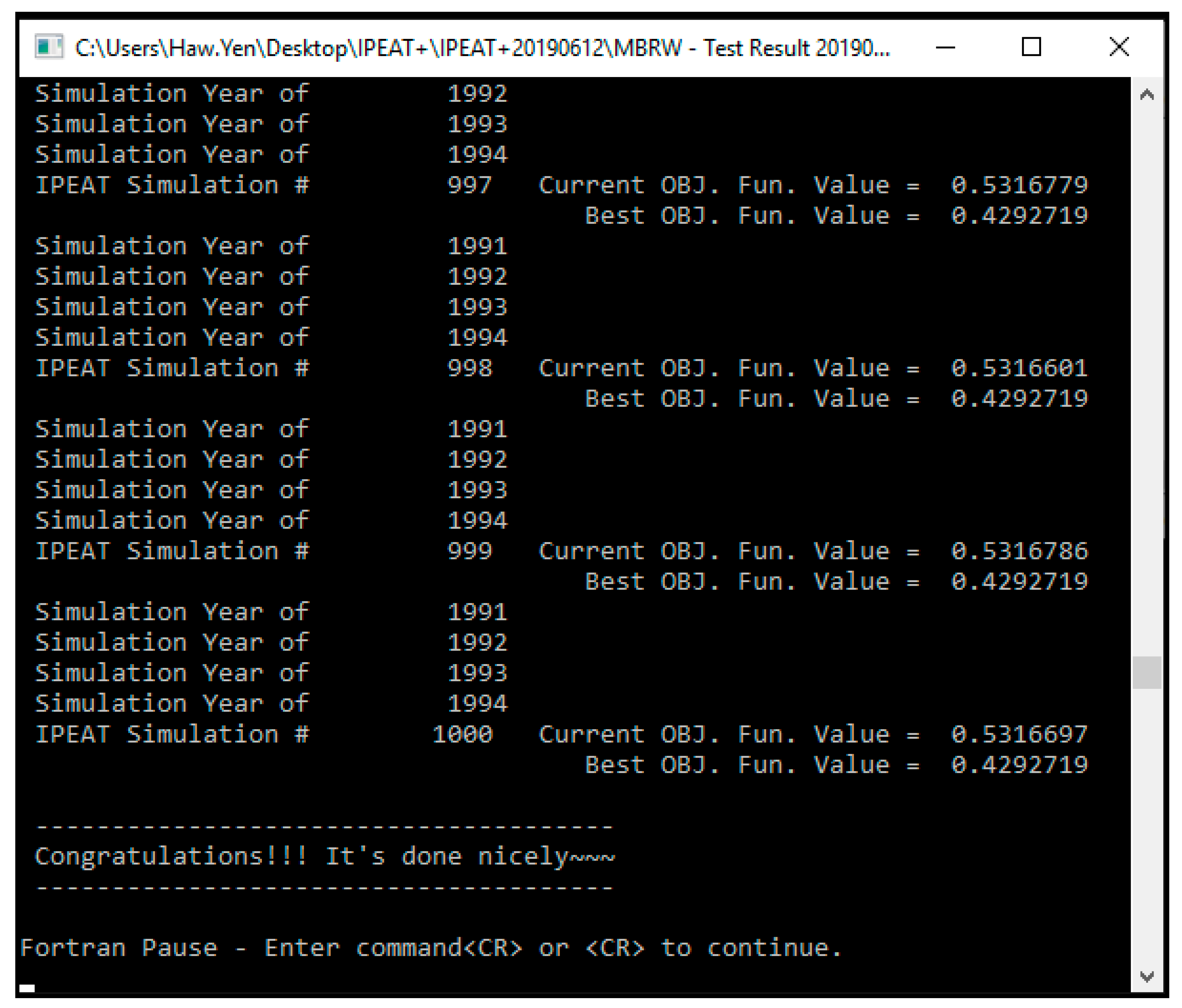
2.4.1. Calibration Parameter Sets and Objective Function Values

As shown in Figure 4a, parameter sets used during calibration and the corresponding objective function values are printed in the order of simulations. Parameters will only be shown for the ones that are being checked in the IPEAT_Para.set (specifically, the “Selection” option). The given objective function values in this file are the integrated sum after multiplying the original objective function by the weights assigned in the IPEAT_Control.set. In addition, some statistics will be transformed (such as NSE and R² are transformed to 1-NSE and 1-R²) to serve the purpose of optimization routines. For example, the potential values of NSE range from 1 (best) to −∞ (worst). One cannot minimize NSE in the original format, and similar issue also applies to R².

2.4.2. Statistical Outputs and Output Processes

In modern day watershed modeling projects, statistical outputs are widely used as quantitative standards to provide scientifically credible guidance in assessing performance of simulation outputs. For example, General Performance Ratings (GPR) is one of the most commonly adopted statistical measurements in the field of water and environmental science [13]. In IPEAT+, five frequently implemented statistics are calculated for each run. On the other hand, users can add more statistics in the code with minor effort. As shown in Figure 4b, statistical results of individual output variable (in this case, 1 = streamflow rate and 2 = sediment load) in each runs are printed in IPEAT_Stats.out. Please note that statistics here are not necessary objective function values for the reasons explained in the previous subsection. In addition to statistical results, modeling output processes in each time step (e.g., daily streamflow) are also saved into a single file (IPEAT_Processes.out in Figure 4c). One can take advantage of information from this file and explore advanced investigation such as uncertainty analysis.

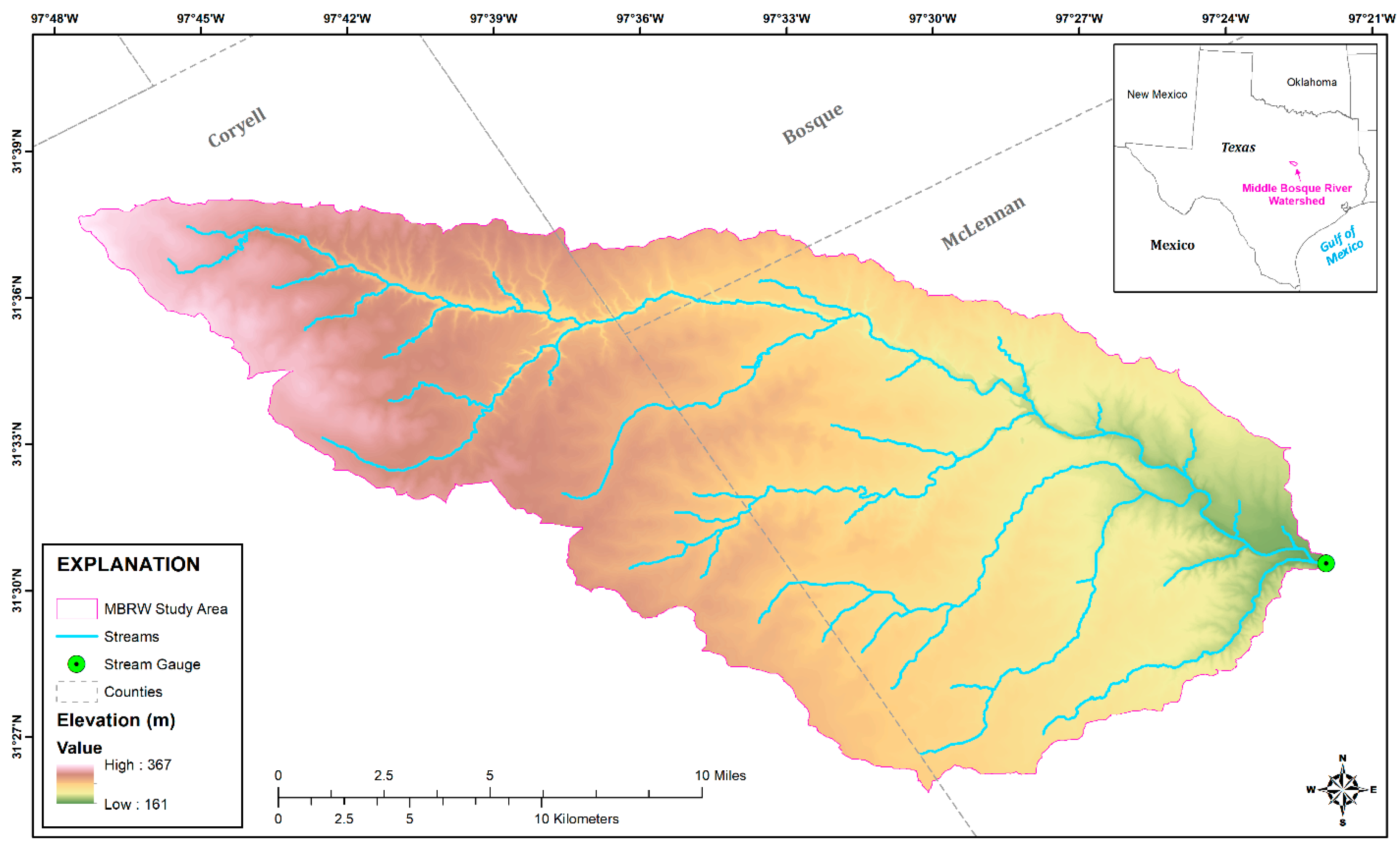
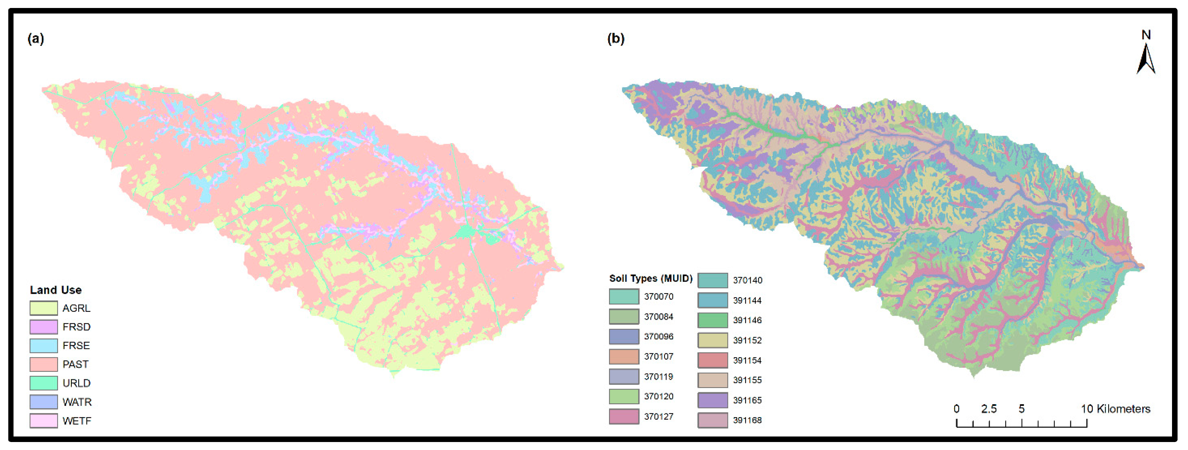
2.5. Study Area and Model Setup of Example Application

The features and capabilities of IPEAT+ are demonstrated through an application to the 471 km² Middle Bosque River Watershed (MBRW) in the Texas-Gulf Region of Central Texas (Figure 5). The MBRW includes portions of McLennan, Bosque, and Coryell counties and its altitude varies from 367 m at the highest point on the northwestern edge to 161 m on the eastern edge. The study region mainly consists of 65.4% pasture and 20.3% farm lands, with minor land covers of 8.5 % forests, and 3.2% residential areas (USGS, 2007) (Figure 6). The climate in the MBRW is characterized as semi-arid, with long hot summers and short mild winters. The warmest month, August, has an average maximum temperature of 36.5 °C while the coldest month, January, has an average minimum temperature of 2.8 °C (U.S. Depth. of Commerce, Weather Bureau, 1980–2012). The average annual precipitation is 1081 mm/year.

For the SWAT+ model setup, the QSWAT+ plugin (Version 0.9) was used with QGIS 2.18.23 (https://qgis.org/en/site/). The required input data to construct the MBRW SWAT+ model are a digital elevation model (DEM), a raster soil map and raster land use map. A total of 69 subbasins were delineated based on the DEM. Using the soil and land-use maps with no threshold setting for the HRU definition, a total of 1721 HRUs was created. As shown in

Table 2. Descriptions of SWAT+ parameters selected for calibration in case study.

Parameters	Input File	Units	Range	Description
awc	sol	mm_H20/mm	±100	Available water capacity of the soil layer
cn2	hru	%	±30	Initial SCS CN II value
delay	gw	Day	0–500	Groundwater delay
epco	hru	-	0–1	Plant uptake compensation factor
esco	hru	-	0–1	Soil evaporation compensation factor
flo_min	gw	mm	±100	Minimum aquifer storage to allow return flow
k	sol	mm/hr	±100	Saturated hydraulic conductivity
revap_co	gw	-	0.02–0.2	Groundwater ‘revap’ coefficient
revap_min	gw	mm	±100	Threshold depth of water in the shallow aquifer required for return flow to occur

, a total of nine SWAT+ parameters were selected for model calibration. In this study, the SWAT+ MBRW project was simulated for daily streamflow process from 1991 to 1994, whereas the first two years were used for warm-up period.

2.6. Performance Evaluation

As mentioned earlier, there are five statistical measures available in IPEAT and IPEAT+ for evaluation of modelling performance. All five statistics will be calculated and stored in the output file (IPEAT_Stats.out). On the other hand, there will be only one objective function used for optimization. Specifically, the aggregate objective function (since the targeted output variable cold be more than one such as flow rate, sediment, and nutrient loads) will be minimized to seek for better fit between observation data and simulation outputs. In this case, one will find that NSE (Equation (1)) cannot be minimized for the nature of potential values range from −∞ (worst fit) to one (perfect match between simulation and observation).

$$\mathrm{NSE}=1-\frac{{{\displaystyle \sum }}_{i=1}^N{\left(y_i^{Obs}-y_i^{Sim}\right)}^2}{{{\displaystyle \sum }}_{i=1}^N{\left(y_i^{Obs}-y_i^{Mean}\right)}^2}$$

(1)

where, $y_i^{Obs}$ is the observation record at time step $i$; $y_i^{Sim}$ is the simulated modeling responses at time step $i$; $y_i^{Mean}$ is the averaged observation record at time step $i$; and $N$ is the number of total simulation time steps. Therefore, NSE has to be slightly transformed to serve the purpose shown in Equation (2) (details can also be found in Seo et al., 2014):

$$OF={{\displaystyle \sum }}_{m=1}^M{\left(1-NS{E}_m^{}\right)}^{}$$

(2)

where, $OF$ is the transformed objective function;$NS{E}_m$ is the NSE value of aggregated modeling responses $m$; and $M$ is the total number of modeling responses (in case study, $M=1$ for streamflow). Note that the best potential value of $OF$ is zero if all $NS{E}_m$ are equal to one. One will find that it is mathematically doable (but not recommended) in IPEAT and IPEAT+ to have an aggregated objective function among different statistical functions (e.g., merge NSE with PBIAS). However, it may not represent statistical robustness since it is hard to identify the true scientific meanings of the aggregated values.

3. Results and Discussion

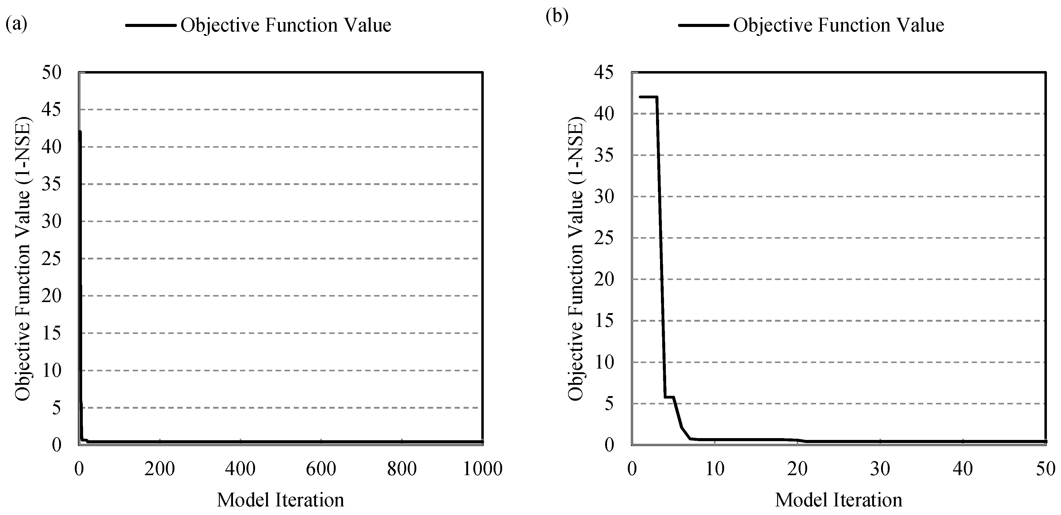
3.1. General Comparisons of Model Performance

As shown in Figure 7a, four years of model simulation using IPEAT+ for 1000 runs can be completed within 4.5 h when a computing system with 64-bit operating system, x64-based processer, Intel® Core™ i7-6700K [email protected], and RAM 32.0 GB was used. For demonstration purpose, a lot more model simulations were conducted to achieve full convergence. In general, it can be identified that calibration converged fairly quickly within 100 runs. It is not surprised to see fast convergence since hydrologic processes are generally easier to simulate in SWAT modeling projects. In addition, the total number of parameters is only nine, which lower than other SWAT projects whereas calibration of more than 50 parameters is not unusual [30].

Beyond the overall objective function values, parameter values and the corresponding converging behavior could be useful to users as well. As shown in Figure 8, users can take this piece of information to further examine the convergence process of each parameter during calibration. For example, in the given outputs, one can find that curve number (cn2) may be under the situation of over-calibration. Curve number values converged very close to the lower bound (−30% in reduction), which is a general indication of over-calibration. One should also note that the given work is an illustrative operation of the IPEAT+ program. Detailed calibration results could vary by changing scenarios.

Comparison of model converging processes may not be very informative in terms of modeling results since objective function can be aggregated in various ways. However, it was stated in the literature that results of model convergence may be useful while users are trying to have a general sense on how the automatic calibration process is executed over time [30]. Users can take advantage of the convergence chart to identify some easy errors taken place in watershed modeling work. For example, fluctuating converging curves or extremely large values of objective function may indicate (but not limited to): (a) Improper selection and settings of model parameters; (b) false default settings in the watershed input files (climate, land use, or soil data); or, (c) mismatching gauge station(s) between observation data versus simulation outlet(s). In IPEAT+, current and the best objective function values will be printed on the MS-DOS command window (see Figure 9) so that users may have early signs before waiting for the full completion (could be thousands of runs after days or weeks).

3.2. Evaluation of Calibrated SWAT+ in Hydrologic Outputs

The best calibration results for the simulation years are reasonably good (NSE: 0.57, PBIAS: −7.70%; and, R²: 0.58). According to GPR statistical reference, the derived results ranged from “Satisfactory” to “Good”. GPR is also termed as behavior definition whereas users and decision makers can take preliminary and timely judgment calls by initial solutions [22]. On the other hand, one cannot fully rely on GPR exclusively since the finalized GPR categories were organized from very limited case studies.

To better understand the performance of the calibrated SWAT+ with IPEAT+, daily outputs of streamflow were plotted on a monthly basis (it’s a lot easier to have better graphical visualization). As shown in Figure 10a, daily streamflow simulations outputs were converted to monthly and the corresponding uncertainty bands were built by using outputs from IPEAT_Processes.out. The primary statistics for monthly flow are slightly better than daily streamflow simulations (NSE: 0.61, PBIAS: 8.39%; and, R²: 0.79). In general, the optimized (calibrated) streamflow simulations and observation data are fairly close. Only the beginning months can be found to have noticeable differences. Longer warm-up period should be applied to resolve this issue. Uncertainty band constructed by using streamflow outputs in each iteration has not shown strong trend in terms of average uncertainty band width (varied substantially in different months) nor clear temporal routines (cannot identify identifiable trend or average width in certain month). As mentioned in earlier work of IPEAT, DDS tends to derive candidate results within relatively narrow ranges [19]. For uncertainty analysis, one should consider to replace DDS with other optimization or mathematical schemes such as Generalized Likelihood Uncertainty Estimation (GLUE) [33] or other Bayesian inferences.

In addition to streamflow processes and uncertainty band, flow duration curves (FDCs) were also generated to examine the model performance. As shown in Figure 10b, the resulting uncertainties in the simulation of short-term average discharge as well as FDCs of daily discharge were analyzed to provide an additional comparison between observed and simulated daily streamflow at the gauge site. The shape and magnitude of the flow duration curve from the IPEAT+ best simulation is similar to the FDCs from the observation data, with flow rates ranging from 10 to 40 m³/s. However, the IPEAT+ best simulation overestimates the mid to low-range flows (<10 m³/s) resulting in simulated flow rates are always greater than or equal to 0.2 m³/s whereas the observation data show that flow rates are less than 10 m³/s exceeded 40% of the time, approximately. There are some possible contributions to the overestimation of the mid to low-range daily flow, i.e., short-term calibration period and small number of parameters used. In addition, selection of objective function could also cause similar issue since NSE has been shown to better capture high flows than low flows. The primary goal of this case study is for demonstration purpose, whereas detailed model calibration and adjustments are out of the scope. On the other hand, the fitting FDCs between observed and simulated streamflow may be improved while IPEAT+ settings fully reconsider calibration period (longer) and number of parameters (more).

4. Conclusions and Future Development

In this study, development of IPEAT+ as an efficient automatic calibration tool coupled with SWAT+ has been presented. Operation of IPEAT+ is fairly easy, where only three primary input files (control file, parameter setting file, and observation data file) are mandatory to conduct automatic calibration routines. For general users (focus on SWAT+ applications), IPEAT+ is a convenient program in which automatic calibration functions are provided along with SWAT+ executable in one piece. It’s not requisite for users to purchase or install any other software for operation. In addition, IPEAT+ is the first automatic calibration tool supported by the SWAT developers group where potential modifications and suggestions can be made via the general SWAT forum and also in regular International SWAT Conferences. For advanced users (focus on SWAT+ development, improvement, and other investigations such as model coupling and uncertainty analysis), the open-source code provides sufficient flexibility for making essential changes in the source code.

Coupling IPEAT+ with SWAT+ is fairly simple, which can be conducted by users with minor efforts. IPEAT+ will be regularly updated with the latest SWAT+ revision. On the other hand, only few lines in the source code (IPEAT+ related codes only needed to be inserted without making any changes) are required to be updated if potential users would like to integrate IPEAT+ with various versions of SWAT+.

The current version of IPEAT+ does not cover uncertainty analysis yet. On the other hand, more development of IPEAT+ will be conducted in the near future so that uncertainty sources such as inputs, parameters, structure, and measurement data can be considered explicitly during the watershed modeling processes. In addition to SWAT+ applications in a singular model, one can take advantage of the simple IPEAT+ framework for model coupling explorations by integrating multiple models. SWAT used to be coupled with other models successfully such as SWAT-MODFLOW [34], SWAT with CE-QUAL-W2 [35], and SWAT-WetQual [36]. More cutting-edge and forward-thinking scientific questions can be answered by far more complex modeling systems.

References

1. Arnold, J.G.; Moriasi, D.N.; Gassman, P.W.; Abbaspour, K.C.; White, M.J.; Srinivasan, R.; Santhi, C.; Harmel, R.D.; Van Griensven, A.; Van Liew, M.W.; et al. SWAT: Model Use, Calibration, and Validation. Trans. ASABE 2012, 55, 1491–1508. [Google Scholar] [CrossRef]
2. Hantush, M.; Kalin, L.; Isik, S.; Yucekaya, A. Nutrient dynamics in flooded wetlands: I. Model development. J. Hydrol. Eng. 2013, 18, 1709–1723. [Google Scholar] [CrossRef]
3. Williams, J.W.; Izaurralde, R.C.; Steglich, E.M. Agricultural Policy/Environmental Extender Model Theoretical Documentation Version 0806; Texas A&M University: College Station, TX, USA, 2012; p. 131. [Google Scholar]
4. Bicknell, B.R.; Imhoff, J.C.; Kittle, J.L., Jr.; Donigian, A.S.; Johanson, R.C. Hydrological Simulation Program--Fortran: User’s Manual for Version 11. U.S.; Environmental Protection Agency, National Exposure Research Laboratory: Athens, GA, USA, 1997; 755p.
5. USDA—Natural Resources Conservation Service (NRCS). Assessment of the Effects of Conservation Practices on Cultivated Cropland in the Great Lakes Region, Conservation Effects Assessment Project (CEAP); United States Department of Agriculture: Washington, DC, USA, 2011.
6. Johnson, M.V.V.; Norfleet, M.L.; Atwood, J.D.; Behrman, K.D.; Kiniry, J.R.; Arnold, J.G.; White, M.J.; Williams, J. The Conservation Effects Assessment Project (CEAP): A national scale natural resources and conservation needs assessment and decision support tool. IOP Conf. Ser. Earth Environ. Sci. 2015, 25, 12012. [Google Scholar] [CrossRef]
7. Scavia, D.; Kalcic, M.; Muenich, R.L.; Read, J.; Aloysius, N.; Bertani, I.; Boles, C.; Confesor, R.; DePinto, J.; Gildow, M.; et al. Multiple models guide strategies for agricultural nutrient reductions. Front. Ecol. Environ. 2017, 15, 126–132. [Google Scholar] [CrossRef]
8. Coffey, R.; Cummins, E.; Bhreathnach, N.; O’Flaherty, V.; Cormican, M. Development of a pathogen transport model for Irish catchments using SWAT. Agric. Water Manag. 2010, 97, 101–111. [Google Scholar] [CrossRef]
9. Yen, H.; Lu, S.; Feng, Q.; Wang, R.; Gao, J.; Brady, D.M.; Sharifi, A.; Ahn, J.; Chen, S.T.; Jeong, J.; et al. Assessment of Optional Sediment Transport Functions via the Complex Watershed Simulation Model SWAT. Water 2017, 9, 76. [Google Scholar] [CrossRef]
10. Yuan, Y.; Wang, R.; Cooter, E.; Ran, L.; Daggupati, P.; Yang, D.; Srinivasan, R.; Jalowska, A. Integrating multimedia models to assess nitrogen losses from the Mississippi River basin to the Gulf of Mexico. Biogeosciences 2018, 15, 7059–7076. [Google Scholar] [CrossRef] [Green Version]
11. Wang, R.; Yuan, Y.; Yen, H.; Grieneisen, M.; Arnold, J.; Wang, D.; Wang, C.; Zhang, M. A review of pesticide fate and transport simulation at watershed level using SWAT: Current status and research concerns. Sci. Total Environ. 2019, 669, 512–526. [Google Scholar] [CrossRef]
12. Feng, Q.; Chaubey, I.; Cibin, R.; Engel, B.; Sudheer, K.P.P.; Volenec, J. Simulating establishment periods of switchgrass and Miscanthus in the soil and water assessment tool (SWAT). Am. Soc. Agric. Biol. Eng. 2017, 60, 1621–1632. [Google Scholar] [CrossRef]
13. Moriasi, D.N.; Arnold, J.G.; Van Liew, M.W.; Bingner, R.L.; Harmel, R.D.; Veith, T.L. Model Evaluation Guidelines for Systematic Quantification of Accuracy in Watershed Simulations. Trans. ASABE 2007, 50, 885–900. [Google Scholar] [CrossRef]
14. Kalin, L.; Isik, S.; Schoonover, J.E.; Lockaby, B.G. Predicting Water Quality in Unmonitored Watersheds Using Artificial Neural Networks. J. Environ. Qual. 2010, 39, 1429–1440. [Google Scholar] [CrossRef]
15. Wang, R.Y.; Bowling, L.C.; Cherkauer, K.A.; Cibin, R.; Her, Y.; Chaubey, I. Biophysical and hydrological effects of future climate change including trends in CO2, in the St. Joseph River watershed, Eastern Corn Belt. Agric. Water Manag. 2017, 180, 280–296. [Google Scholar] [CrossRef] [Green Version]
16. Guo, T.; Engel, B.A.; Shao, G.; Arnold, J.G.; Srinivasan, R.; Kiniry, J.R. Development and improvement of the simulation of woody bioenergy crops in the Soil and Water Assessment Tool (SWAT). Environ. Model. Softw. 2018. [Google Scholar] [CrossRef]
17. Guo, T.; Gitau, M.; Merwade, V.; Arnold, J.; Srinivasan, R.; Hirschi, M.; Engel, B. Comparison of performance of tile drainage routines in SWAT 2009 and 2012 in an extensively tile-drained watershed in the Midwest. Hydrol. Earth Syst. Sci. 2018, 22, 89–110. [Google Scholar] [CrossRef] [Green Version]
18. Abbaspour, K.C.; Yang, J.; Maximov, I.; Siber, R.; Bogner, K.; Mieleitner, J.; Zobrist, J.; Srinivasan, R. Modelling hydrology and water quality in the pre-alpine/alpine Thur watershed using SWAT. J. Hydrol. 2007, 333, 413–430. [Google Scholar] [CrossRef]
19. Yen, H.; Bailey, R.T.; Arabi, M.; Ahmadi, M.; White, M.J.; Arnold, J.G. The Role of Interior Watershed Processes in Improving Parameter Estimation and Performance of Watershed Models. J. Environ. Qual. 2014, 43, 1601–1613. [Google Scholar] [CrossRef]
20. Arnold, J.G.; Bieger, K.; White, M.J.; Srinivasan, R.; Dunbar, J.A.; Allen, P.M. Use of Decision Tables to Simulate Management in SWAT+. Water 2018, 10, 713. [Google Scholar] [CrossRef]
21. Wang, X.; Yen, H.; Liu, Q.; Liu, J. An auto-calibration tool for the Agricultural Policy Environmental eXtender (APEX) model. Trans. ASABE 2014, 57, 1087–1098. [Google Scholar] [CrossRef]
22. Yen, H.; Wang, X.; Fontane, D.G.; Harmel, R.D.; Arabi, M. A framework for propagation of uncertainty contributed by parameterization, input data, model structure, and calibration/validation data in watershed modeling. Environ. Model. Softw. 2014, 54, 211–221. [Google Scholar] [CrossRef]
23. Arnold, J.G.; Williams, J.R.; Maidment, D.R. Continuous-Time Water and Sediment-Routing Model for Large Basins. J. Hydraul. Eng. 1995, 121, 171–183. [Google Scholar] [CrossRef]
24. Williams, J.R.; Nicks, A.D.; Arnold, J.G. Simulator for Water Resources in Rural Basins. J. Hydraul. Eng. 1985, 111, 970–986. [Google Scholar] [CrossRef]
25. Daggupati, P.; Yen, H.; White, M.J.; Srinivasan, R.; Arnold, J.G.; Keitzer, C.S.; Sowa, S.P. Impact of model development, calibration and validation decisions on hydrological simulations in West Lake Erie basin. Hydrol. Process. 2015, 29, 5307–5320. [Google Scholar] [CrossRef]
26. Keitzer, S.; Ludsin, S.A.; Sowa, S.; Annis, G.; Daggupati, P.; Froelich, A.M.; Herbert, M.E.; Johnson, M.V.; Yen, H.; White, M.J.; et al. Thinking outside the lake: How might Lake Erie nutrient management benefit stream conservation in the watershed? J. Great Lakes Res. 2016, 42, 1322–1331. [Google Scholar] [CrossRef]
27. Yen, H.; Jeong, J.; Smith, D.R. Evaluation of Dynamically Dimensioned Search Algorithm for Optimizing SWAT by Altering Sampling Distributions and Searching Range. JAWRA J. Am. Water Resour. Assoc. 2016, 52, 443–455. [Google Scholar] [CrossRef]
28. Worqlul, A.W.; Ayana, E.K.; Yen, H.; Jeong, J.; MacAlister, C.; Taylor, R.; Gerik, T.J.; Steenhuis, T.S. Evaluating hydrologic responses to soil characteristics using SWAT model in a paired-watersheds in the Upper Blue Nile Basin. Catena 2018, 163, 332–341. [Google Scholar] [CrossRef]
29. Soil and Water Assessment Tool Literature Database. Available online: http://swatmodel.tamu.edu (accessed on 14 July 2019).
30. Yen, H.; Jeong, J.; Tseng, W.H.; Kim, M.K.; Records, R.M.; Arabi, M. Computational Procedure for Evaluating Sampling Techniques on Watershed Model Calibration. J. Hydrol. Eng. 2015, 20, 04014080. [Google Scholar] [CrossRef]
31. Yen, H.; White, M.J.; Arnold, J.G.; Keitzer, S.C.; Johnson, M.V.V.; Atwood, J.D.; Daggupati, P.; Herbert, M.E.; Sowa, S.P.; Ludsin, S.A.; et al. Western Lake Erie Basin: Soft-data-constrained, NHDPlus resolution watershed modeling and exploration of applicable conservation scenarios. Sci. Total Environ. 2016, 569, 1265–1281. [Google Scholar] [CrossRef]
32. Nash, J.; Sutcliffe, J. River flow forecasting through conceptual models part I—A discussion of principles. J. Hydrol. 1970, 10, 282–290. [Google Scholar] [CrossRef]
33. Beven, K.; Binley, A. The future of distributed models: Model calibration and uncertainty prediction. Hydrol. Process. 1992, 6, 279–298. [Google Scholar] [CrossRef]
34. Bailey, R.T.; Wible, T.C.; Arabi, M.; Records, R.M.; Ditty, J. Assessing regional-scale spatio-temporal patterns of groundwater-surface water interactions using a coupled SWAT-MODFLOW model. Hydrol. Process. 2016, 30, 4420–4433. [Google Scholar] [CrossRef]
35. Jeong, J.; Wagner, K.; Flores, J.J.; Cawthon, T.; Her, Y.; Osorio, J.; Yen, H. Linking watershed modeling and bacterial source tracking to better assess E. coli sources. Sci. Total Environ. 2019, 648, 164–175. [Google Scholar] [CrossRef]
36. Haas, H.; Isik, S.; Kalin, L.; Hantush, M. Studying Impacts of Wetlands in Fish River Watershed Nutrient Export through coupling of SWAT and WetQual. In Proceedings of the EWRI Congress, Pittsburgh, PA, USA, 19–23 May 2019. [Google Scholar]
Figure 1. Computational framework of IPEAT+ with SWAT+ in watershed modeling.
Water 11 01681 g001
Figure 2. Illustration of IPEAT+ input files: IPEAT_Control.set with required settings.
Water 11 01681 g002
Figure 3. Illustration of IPEAT+ input files: (a) parameter setting file for automatic calibration in IPEAT_Para.set; and, (b) example of observation data file at daily time step.
Water 11 01681 g003
Figure 4. Illustration of IPEAT+ output files: (a) Parameter outputs for calibration parameter sets and the corresponding objective function values; (b) statistical results of individual output variable in each runs (NSE: Nash-Sutcliffe Efficiency Coefficient; PBIAS: Percent Bias; RMSE: Root Mean Square Error; R2: Coefficient of Determination; and, MSE: Mean Squared Error); and, (c) modeling output processes of targeted output variable.
Water 11 01681 g004
Figure 5. Location of Middle Bosque River Watershed, located in the Texas-Gulf Region of Central Texas.
Water 11 01681 g005
Figure 6. Geographical inputs for HRU definition in SWAT+: (a) land use; and, (b) soil types.
Water 11 01681 g006
Figure 7. General model performance and the convergence of objective function values: (a) full calibration process of 1000 iterations; and, (b) closer look of the first 50 runs.
Water 11 01681 g007
Figure 8. Convergence progression (1000 model iterations) and the corresponding values (with upper and lower bounds) of nine model parameters selected for calibration. Solid red lines represent the converged value of calibrated parameters.
Water 11 01681 g008
Figure 9. MS-DOS Command window of IPEAT+ execution with the latest updates on current and the best objective function values.
Water 11 01681 g009
Figure 10. Hydrologic processes of the calibrated SWAT+ model by using IPEAT+: (a) Monthly average observed and best simulated time series of stream discharge; (b) daily observed and best simulated Flow Duration Curves, with simulated uncertainties resulting from the 1000 combinations of IPEAT+ ensemble parameter set for the Middle Bosque River watershed.
Water 11 01681 g010