Removal of Diesel Oil in Soil Microcosms and Implication for Geophysical Monitoring


1
Department of Applied Science and Technology, Politecnico di Torino, Corso Duca degli Abruzzi 24, 10129 Torino, Italy
2
Department of Environment, Land and Infrastructure Engineering, Politecnico di Torino, Corso Duca degli Abruzzi 24, 10129 Torino, Italy
*
Author to whom correspondence should be addressed.
Water 2019, 11(8), 1661; https://doi.org/10.3390/w11081661
Submission received: 30 May 2019
/
Revised: 3 August 2019
/
Accepted: 8 August 2019
/
Published: 11 August 2019
(This article belongs to the Special Issue Technological Eco-Innovations for the Quality Control and the Decontamination of Polluted Waters and Soils)
Abstract
:Bioremediation of soils polluted with diesel oil is one of the methods already applied on a large scale. However, several questions remain open surrounding the operative conditions and biological strategies to be adopted to optimize the removal efficiency. This study aimed to investigate the environmental factors that influence geophysical properties in soil polluted with diesel oils, in particular, during the biodegradation of this contaminant by an indigenous microbial population. With this aim, aerobic degradation was performed in soil column microcosms with a high concentration of diesel oil (75 g kg−1 of soil); the dielectric permittivity and electrical conductivity were measured. In one of the microcosms, the addition of glucose was also tested. Biostimulation was performed with a Mineral Salt Medium for Bacteria. The sensitivity of the dielectric permittivity versus temperature was analyzed. A theoretical approach was adopted to estimate the changes in the bulk dielectric permittivity of a mixture of sandy soil-water-oil-gas, according to the variations in the oil content. The sensitivity of the dielectric permittivity to the temperature effects was analyzed. The results show that (1) biostimulation can give good removal efficiency; (2) the addition of glucose as a primary carbon source does not improve the diesel oil removal; (3) a limited amount of diesel oil was removed by adsorption and volatilization effects; and (4) the diesel oil efficiency removal was in the order of 70% after 200 days, with different removal percentages for oil components; the best results were obtained for molecules with a low retention time. This study is preparatory to the adoption of geophysical methods to monitor the biological process on a larger scale. Altogether, these results will be useful to apply the process on a larger scale, where geophysical methods will be adopted for monitoring.
1. Introduction
Soil pollution has an anthropogenic origin, often due to accidental or improper industrial spills, stockpile leakages, improper waste disposal, mining, and military activities, to name just a few examples. Looking at the contaminant classes, most of them are mineral oils, heavy metals, metalloids or organic compounds, due to hydrocarbon leakages in the subsoil and groundwater.
Diesel oil is widely used in many industrial sectors, mainly for transport and energy plants, and therefore it is one of the common soil pollutants, with huge impacts on human health, the environment, and economy. For its removal, in situ bioremediation is considered an environmentally friendly and cost-effective solution, due to the metabolic capability of microorganisms to degrade the pollutants. So far, bioremediation is performed by means of
- bioaugmentation: The addition of enriched microbial cultures (autochthonous or allochthonous degraders) to the soil [3];
Several studies were carried out in different operative conditions, adopting one of the aforesaid strategies, and aimed to optimize hydrocarbon removal [3,6,7,8,9]. It is widely known that biostimulation is an easier process to carry out [2,5,10,11]. However, when biostimulation does not give satisfactory results, bioaugmentation is adopted, or coupled methods are applied.
In a previous study carried out with the same soil contaminated with a commercial diesel oil (7.5% w/w soil) [12], the effect of biostimulation was investigated. The results clearly showed that the medium favoring bacterial growth was more effective in promoting indigenous microbial activity (in terms of CO2 production and biomass dry weight). In a subsequent work [13], the biodegradation efficiencies of biodegradation with and without the addition of a primary carbon source (e.g., glucose) were compared. The results in the biostimulated and bioaugmented microcosms were very similar. It was confirmed that biostimulation can be adopted as a strategy to remove aerobically high concentrations of diesel oil.
In the present study, which is part of a project aiming to apply geophysical methods to monitor the biodegradation of diesel oil in soils, biostimulation was used to remove a high concentration of pollutant (75 g kg−1 of soil). The process was performed by aerobic indigenous microorganisms with and without the addition of a primary carbon source (glucose). The study aimed to better understand if diesel oil removal could be improved by biostimulation of indigenous bacteria; moreover, the contribution of the soil itself to the overall removal was tested.
Kinetic modelling was also performed in order to predict the process performance when transferring the system to a field scale, where geophysical monitoring could be adopted as a fast tool to monitor the behavior of biostimulation.
The challenging issue was to characterize and monitor changes in hydrological and biogeochemical properties/processes, using geophysical measurements at both the laboratory column and field scales. This issue impacts the design of remediation schemes, and it is relevant to check the remediation performances at many contaminated sites. Particularly, at the field scale, the most commonly adopted methods are electrical resistivity, induced polarization, and georadar [14,15]. However, research in bio-geophysics focusses on how microbial growth and biofilm formation could have a potential direct impact on changes in geophysical properties, such as in frequency dependent dielectric permittivity [16]. Moreover, rock texture, surface area, porosity, pore size and shape geometry, tortuosity, formation factor, cementation, and mechanical properties could affect the electromagnetic properties of the soil.
In designing laboratory experiments and geophysical monitoring, a crucial issue is to evaluate how environmental factors could affect geophysical properties; particularly, the dielectric permittivity and electrical conductivity are sensitive to temperature effects. Many authors discussed the effect of temperature both on the dielectrical permittivity and the electrical conductivity of soil; Or and Wraith [17] discussed the role of temperature in complex dielectric permittivity, observed by using time domain reflectometry. The temperature coefficients for both dielectric permittivity and conductivity depend on the mixture composition, the frequency, and the temperature range, and they are useful to compensate for the effect of temperature change during measurements.
At a given frequency and for small temperature changes, the dielectric properties of a mixture vary according to linear temperature coefficients, defined as the percent change in either permittivity or conductivity per Celsius degree. The linear temperature coefficients are limited to a number of specific discrete frequencies and temperatures; outside of these ranges, the temperature impact on the dielectric properties may no longer be linear [18].
Generally, the relative dielectric permittivity and electrical conductivity trends with temperature differ in terms of frequency: In the microwave frequency range, the change in relative permittivity is 2% per Celsius degree and the change in conductivity is between 1 and 2% per Celsius degree, depending on the mixture and on the frequency and temperature range considered.
In such a context, one of the aims is to study/define the sensitivity of dielectric permittivity to the biodegradation of diesel oil in a laboratory column. Starting from the results of microcosm experiments, the analysis of the expected response of the dielectric permittivity during the diesel oil removal, over time, can be carried out.
Dielectric permittivity is a basic electromagnetic property, controlling the radio-wave propagation into the soil, and it is the parameter involved in georadar (GPR) investigation or in Time Domain Reflectometry (TDR) monitoring. Laboratory measurements on sandy soil saturated in water or in diesel oil are found in the literature (e.g., [19]), while time-lapse monitoring of the dielectric permittivity changes caused by oil degradation are less common.
Theoretical models were proposed to describe the contaminant fluid behavior and its effects on dielectric permittivity; for instance, Endres and Redman [20] developed a pore-scale fluid model for clay-free granular soils. In order to predict the characteristics of the hydrocarbon spill, Carcione and Seriani [21] proposed a model for the complex permittivity of a soil composed of sandy grains, clay and silt, partially saturated with gas (air), water, and hydrocarbon. The theory is based on the self-similar model [22,23]. At radar frequencies of 10 MHz–2 GHz, the interfacial and electrochemical mechanisms, such as surface effects, associated with the soil/water interface can be neglected [24]. More recently, multiphase models were implemented for estimating the dielectric permittivity of a mixture of soil-water-gas and oil; the models were validated by using an experimental set-up based on Time Domain Reflectometry (TDR) [25], which is very similar to the approach adopted in our study.
In this study, we focus on the dielectric permittivity of a soil-water-diesel, oil-gas system by evaluating the sensitivity of state-of-art geophysical tools to monitor the degradation effect over time.
2. Materials and Methods
2.1. Soil Properties
The soil was the same as that used for a previous study [13] and was collected in Trecate (Northern Italy), near a site polluted with a crude oil spill. Previous analyses established that the presence of crude oil was not detectable [14].
The soil was sieved and material within the range 0.2–2 mm was used for the study, after oven drying at 70 °C. It should be noted that in its original condition, this soil has a very low water content, which is negligible.
The chemical and physical soil properties are shown in Table 1.
The analysis of the Total Organic Carbon of the soil evidenced a negligible content (<0.1% by weight). The external carbon source was due to diesel oil or to diesel oil and glucose.
2.2. Soil Microcosms
Microcosms were set up in four closed Plexiglas columns (diameter = 0.05 m; height = 0.4 m), each filled with 200 g of soil (layer height = 0.07 m) and operated with different conditions, namely:
- Control abiotic microcosm (A): Sterilized soil, spiked with 15 g of commercial diesel oil and hydrated with 37 mL of sterilized water to obtain a soil moisture level of about 15 % by weight; the sterilization was carried out in an autoclave, at 120 °C for 2 h;
- control biotic microcosm (C): Soil hydrated with 37 mL of Mineral Salt Medium for Bacteria (MSMB);
- biostimulated microcosm (BIOS): Soil treated with 15 g of diesel oil and hydrated with 37 mL of MSMB;
- biostimulated microcosm with added glucose (BIOS-G): The addition of 0.74 g of glucose to 200 g of soil treated with 15 g of diesel oil and hydrated with 37 mL of MSMB; after 143 days, the same amount of glucose was added again.
Soil water content was monitored at time t = 0, 15, 68, 110, 135, 143, and 175 days. After 143 days, 37 mL of MSMB was added to microcosms C, BIOS, and BIOS-G, and the same amount of sterilized water was added to microcosm A.
Each column was opened every 3–4 days to aerate the microcosm. For microcosm A, all the operations were carried out under biological hood.
2.3. Respirometric Measurements
The respirometric activity of the soil microbial population, as CO2 evolution, was measured by CO2 absorption in NaOH solution, using the method described by Bosco et al. [13].
In each microcosm, the measurement was performed every 3–4 days until 218 days.
2.4. Microbial Counts
Soil samples of each microcosm were taken at t = 34, 68, 110, and 175 days to perform the viable microbial count on Malt Extract Agar (MEA) plates, in line with the method used by Bosco et al. [13]. The colony counting was performed after 3 days, and the results were expressed as the number of Colony Forming Units (CFU) per gram of soil.
2.5. Residual Diesel Oil Concentration
In each microcosm, the residual diesel oil concentration was measured by gas-chromatographic analysis of the extract, according to the EPA method 8015. The gas chromatograph (GF) was equipped with a flame ionization detector (FID) and a DB-5 fused silica capillary column, operated with helium gas as the carrier. For the oven, the following temperature program was adopted: Maintaining at 50 °C for 1 min, heating by 8 °C min−1 up to 320 °C and maintaining at 320 °C for 10 min, with a total retention time of 45 min. The injector and detector were maintained at 220 and 280 °C, respectively. The injected extract volume was 1 µL in splitless mode. The residual diesel oil concentration was calculated using a calibration curve obtained with the same commercial diesel oil.
The analyses were performed at different times (0, 15, 68, 110, 135, 175, and 203 days). For each sampling, one sample was taken, and two extracts were prepared and analyzed in triplicate with the aforesaid GC-FID procedure. The gas chromatograms were analyzed as follows:
- The chromatogram from 0 to 8 min was not considered due to the presence of solvent peaks.
- The final part, from 35 to 45 min, was also excluded due to the presence of very small and not well-defined peaks.
- The residual retention time, from 8 to 35 min, was divided into three equal periods, and the corresponding species were classified as:
- ○
- Low retention (LR species), in the period 8–17 min.
- ○
- Medium retention (MR species), in the period 17–26 min.
- ○
- High retention (HR species), in the period 26–35 min.
In each period, the cumulative concentration was calculated as for the total residual one.
2.6. Kinetic Modeling
As for common chemical reactions, the kinetics of hydrocarbon biodegradation can be described with the general model of differential rate law:
where r is the reaction rate, C is the residual reagent concentration, t is time, k is the reaction rate constant, and n is the reaction order.
r = dC/dt = −kCn
Notwithstanding the broad spectrum of possibilities for the reaction order, for bioremediation the most commonly used models are the first-order (n = 1) and the second-order (n = 2), since they give satisfactory results, and their use is rather simple. Therefore, these two models were tested with the data.
2.6.1. First-Order Reaction Rate
In the bioremediation of hydrocarbon-polluted soil, several authors showed the reliability of the first-order reaction rate model [8,26,27,28]. For this model, Equation (1) becomes
r = dC/dt = −kC
Adapting this model to diesel oil biodegradation, it can be assumed that the diesel oil is the key reagent. By integration, the following expression is achieved:
where C(t) is the residual diesel oil concentration at time t (mg kg−1 of soil), C0 is the initial diesel oil concentration (mg kg−1 of soil), k is the reaction rate constant (day−1), and t is time (day).
C(t) = C0 exp (−kt)
The kinetic rates are often expressed in terms of half-life time t1/2, meaning the time by which the starting concentration is halved: At t = t1/2, C = C0/2. Therefore, rearranging Equation (3), it is possible to write and define the half-life time as
t1/2 = ln 2/k = 0.693/k
2.6.2. Second-Order Reaction Rate
Some authors modeled their experimental data for hydrocarbon bioremediation with the second-order reaction rate [29,30].
In this case, with n = 2, Equation (1) becomes
r = dC/dt = −kC2
The solution is
with the half-life time, t1/2:
1/C(t) = 1/C0 + kt
t1/2 = 1/(kC0).
2.7. Geophysical Features for Future Monitoring and Preliminary Measurements
The sensitivity of the bulk dielectric permittivity to changes in the mass of each single element of the materials in the column is checked with the Complex Refractive Index Model (CRIM) (e.g., [25]). This model allows us to predict the bulk dielectric permittivity by accounting for the contribution of each fraction; it was widely adopted to predict the dielectric permittivity of multiphase systems (e.g., Reference [19]). The general formulation of the CRIM model, modified after Knigths and Endres [24], is given by the following formula:
where ϕ is the soil porosity, and Sw and So are the water and oil saturation, respectively, while ε defines the dielectric permittivity of the different materials. The α-exponent accounts for non-linear effects of the interaction between different phases of the mixture. The typical range of the α-exponent is 0.25–0.6.
The simulation was carried out on the same sandy soil adopted for the experiment, with the following assumptions:
- Average porosity: 0.38–0.4;
- soil density: 2700 kg m−3;
- diesel oil density: 800 kg m−3;
- water saturation: 0.4;
- diesel oil concentration equal to 76,000 mg kg−1 of soil, equivalent to diesel oil volume of 0.25 m3 m−3 of the total volume (the mixture oil-water-soil-air);
- water relative electrical permittivity equal to 78 (the water salinity was not considered).
The values and the adopted methodology to estimate the dielectric permittivity of each single component of the mixture are given in Table 2.
3. Results
3.1. Respirometric Measurements
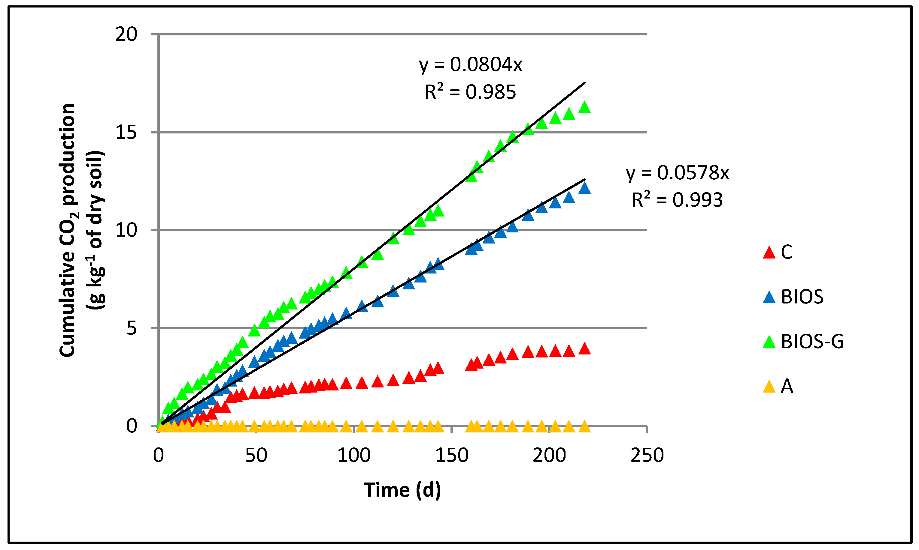
The respirometric activity, expressed as the cumulative amount of CO2 produced in all the tested microcosms, is reported in Figure 1. The main results are the following:
- The control abiotic microcosm (A) had no respirometric activity, as expected.
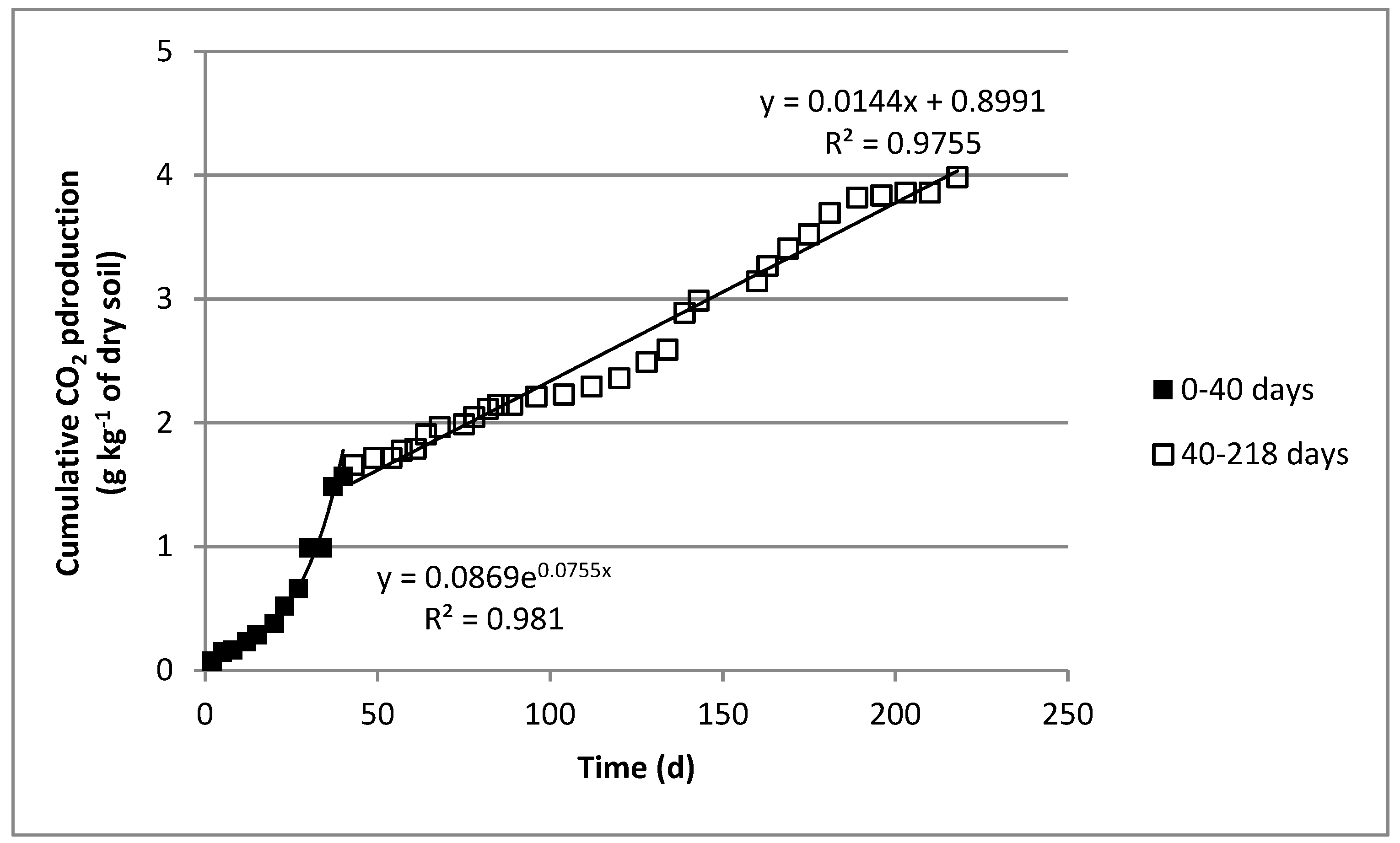
- The control biotic microcosm (C) had the highest respirometric activity in the first 35–40 days, with an exponential trend, then, the daily CO2 production continued but with a reduced amount (Figure 2). After 40 days, the cumulative CO2 quantity grew with an almost linear tendency, demonstrating that the daily production was almost constant and in the order of 0.014 g CO2 kg−1 of soil day−1. In both cases, the regression coefficient R2 had values very close to 1.
- For the BIOS-G microcosm, a slight deviation from linearity occurred at the beginning of the run, when the microbial activity was probably enhanced by the glucose presence, due to the quick use of this primary carbon source with respect to the use of more complex molecules.
- Both biostimulated microcosms, namely without (BIOS) and with glucose (BIOS-G), had cumulative production of CO2 with linear growth, around 0.058 g CO2 kg−1 of soil day−1 and 0.080 g CO2 kg−1 of soil day−1, respectively. These amounts contained the biotic quantity measured in microcosm C, to say the amount naturally produced by the microbial activity in the absence of diesel oil and glucose.
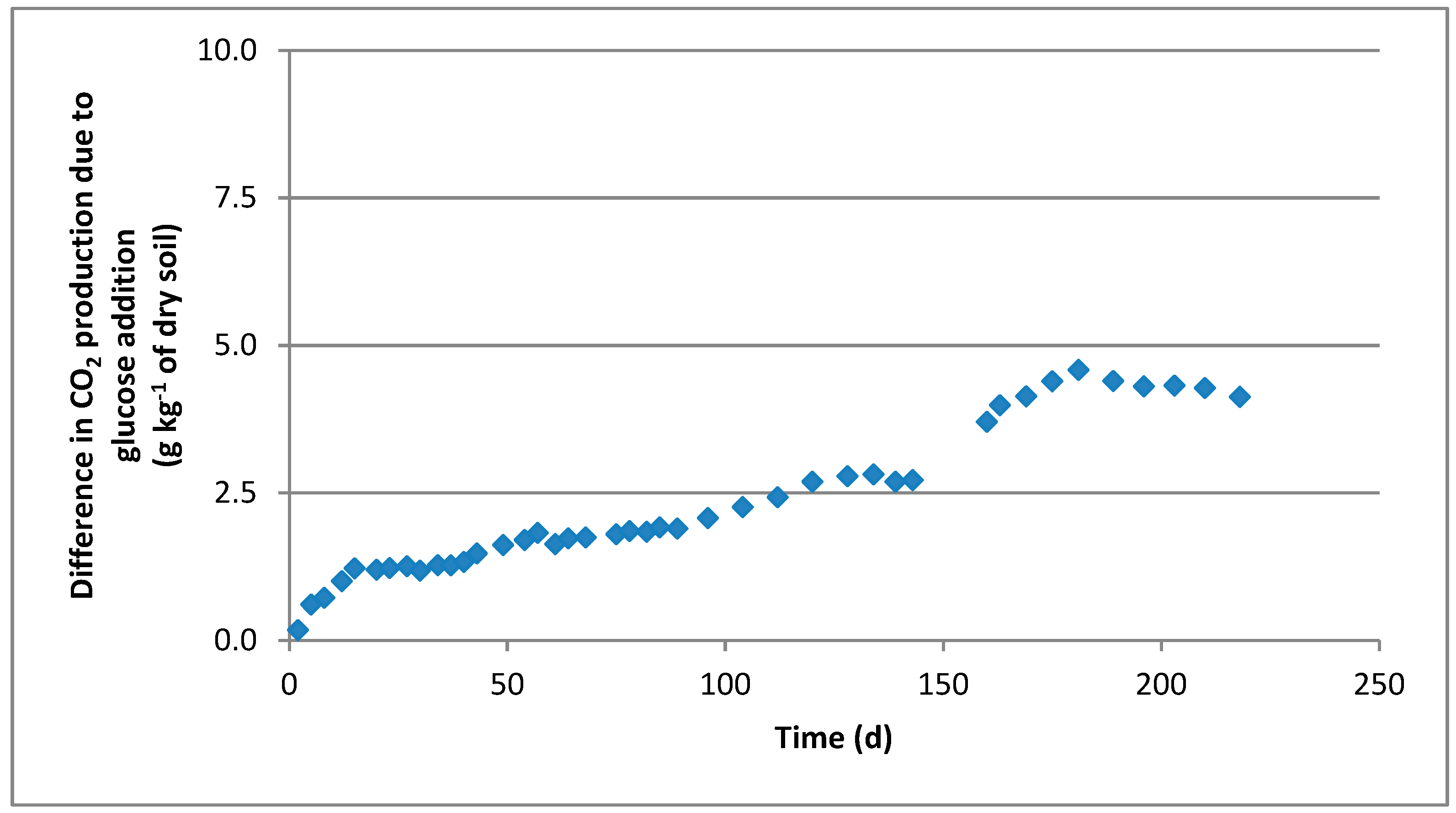
- Comparing the CO2 production of the BIOS and BIOS-G microcosms, the system with added glucose (BIOS-G) produced a higher amount, especially at the beginning of the test, and the difference increased until about 110 days, when the value was in the order of 2.4–2.5 g CO2 kg−1 of soil (Figure 3). This trend was also found after the second addition of glucose to BIOS-G at t = 143 days, when the BIOS-G microcosm started to produce CO2 more quickly than the BIOS microcosm (this feature ended at 163–165 days).
- Without any external addition of carbon sources (microcosm C), the soil had relevant microbial activity: Compared to the cumulative amount achieved in the others, its weight was around 25% of the amount produced when just diesel oil was present (BIOS) and around 17% of the cumulative quantity produced in BIOS-G.
3.2. Microbial Counts
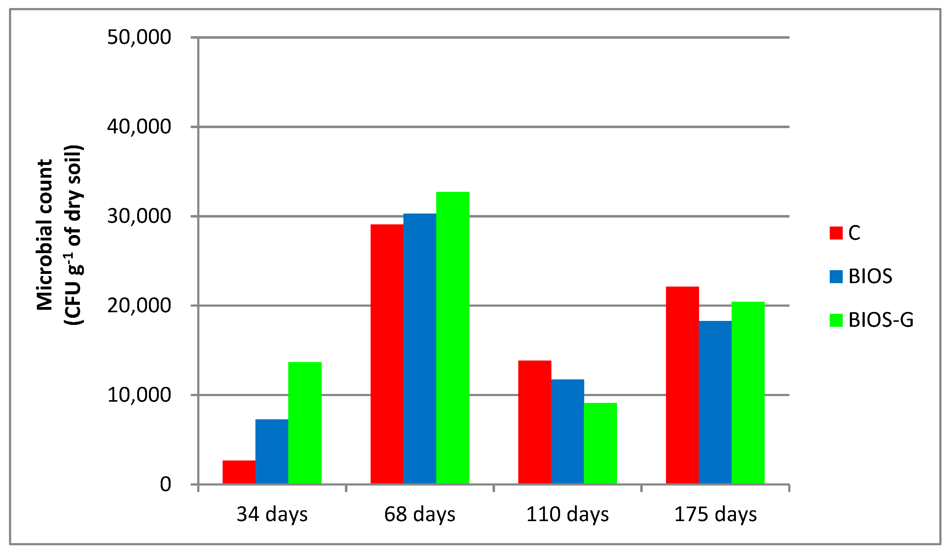
Figure 4 shows the microbial counts obtained on MEA, at different times, in the C, BIOS, and BIOS-G microcosms. We observed that the BIOS-G microcosm had the highest number of colonies during the first two months. The population growth was enhanced by glucose, which as the primary carbon source was metabolized rapidly. For the BIOS-G microcosm, the addition of glucose at t = 143 days apparently influenced the microbial population, which at t = 175 days was more than twice that found at t = 110 days. However, growth also occurred for the C and BIOS microcosms, therefore the addition of MSMB seemed to enhance the growth more than glucose itself.
Among the microcosms, the control one (C) showed the highest value both at 110 days and at 175 days (at 175 days, the population was 60% higher than that found at 110 days). A very similar population growth (around 60%) was achieved in the BIOS microcosm from 110 to 175 days.
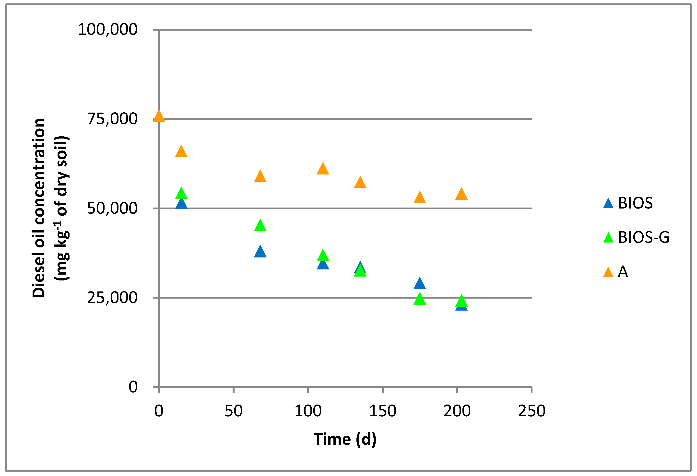
3.3. Diesel Oil Removal
The monitoring of diesel oil content is presented in Figure 5 for the microcosms treated with diesel oil at an initial concentration equal to 75,926 mg diesel oil kg−1 of soil.
During the biodegradation tests, the residual contaminant concentration was measured after 15, 68, 110, 135, 175, and 203 days.
As far as the residual diesel oil concentration in soil is concerned, the following considerations can be pointed out:
- At the end of the test (t = 203 days), in the abiotic microcosm the residual concentration was around 50,000 mg kg−1 of soil, corresponding to a removal efficiency in the order of 30%.
- After 200 days, for the BIOS and BIOS-G microcosms the removal efficiency was very similar and almost 70%, suggesting that the presence of a primary carbon source had no effect on the diesel oil biodegradation. This confirmed the results obtained in a previous work [13] carried out in the same conditions (i.e., biostimulation) but with a different microcosm volume.
- The data shown for the BIOS and BIOS-G microcosms included the abiotic contribution (value obtained in microcosm A); therefore, the net diesel oil removal due to biodegradation was the difference between the overall and abiotic values.
- For the BIOS and BIOS-G microcosms, the trend of residual diesel oil concentration was still decreasing after 200 days; however, this became almost negligible and not substantial in real-case applications.
To better understand the biodegradation and removal process as a whole, in each microcosm, the composition of the residual diesel oil was analyzed and the results compared to the initial one. This information is useful to roughly estimate the removal capability of the process carried out in similar operative and soil conditions.
The results are reported in Figure 6, Figure 7 and Figure 8, for the abiotic, BIOS, and BIOS-G microcosms, respectively.
The removal of LR species was around 57% of the initial content (Figure 6). This occurred rather rapidly, and after about two months the LR species concentration remained at around 15,000 mg kg−1 of soil.
For MR and HR species, very limited removal was achieved. This means that the removal in the abiotic microcosm was mainly for LR species, representative of simple molecules, like aliphatic ones.
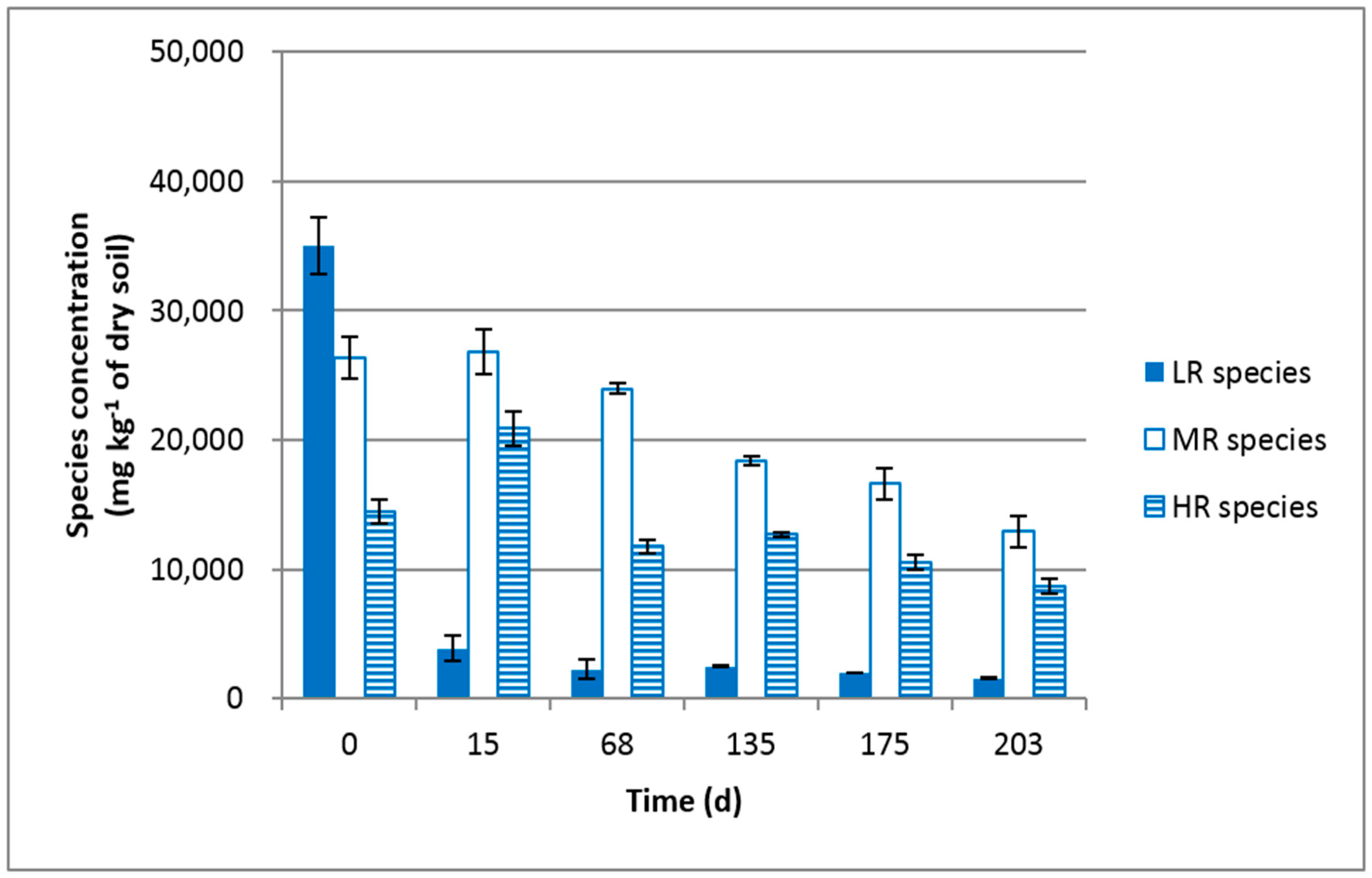
For the BIOS microcosm, the results are shown in Figure 7. In this case, it is possible to observe a different behavior:
- For LR species, after 15 days their concentration was greatly reduced, and after 68 days, the value remained about constant, at around 2000 mg kg−1 of soil. The trend was similar to that shown by the abiotic system, but the constant value was much lower, evidencing that part of these compounds were metabolized by the diesel oil-degrading microorganisms (the LR species contained more quickly biodegradable molecules).
- The removal of MR species was slower and with a lag phase, which could be estimated at two months, since after only 68 days the MR species concentration started to slowly decrease with a trend still continuing at t = 203 days.
- Regarding HR species, the removal was not consistent and seemed to occur slowly with long time durations.
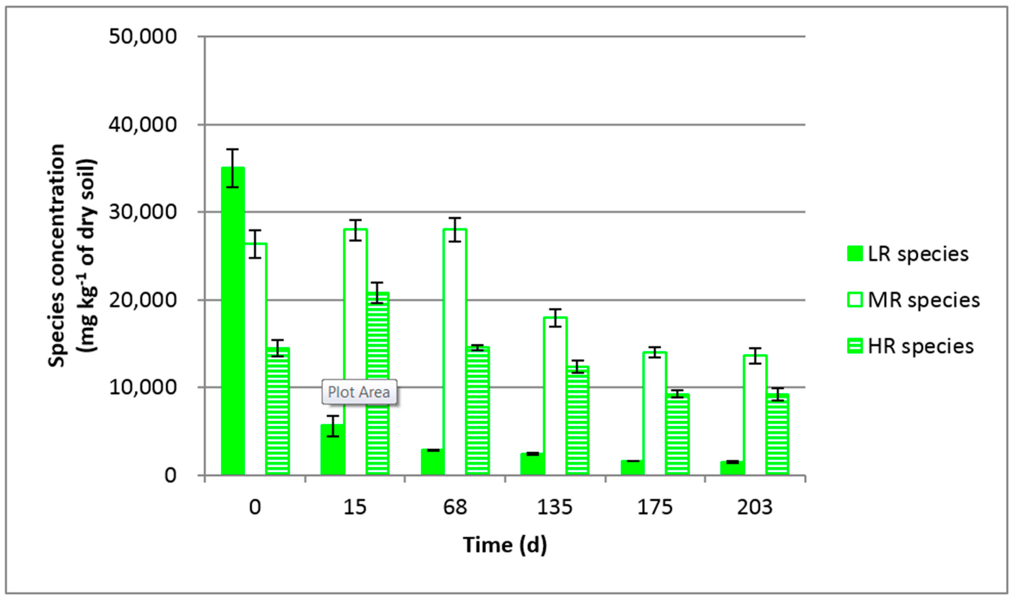
The monitoring of the BIOS-G microcosm (Figure 8) shows results very similar to those obtained with the BIOS microcosm, coherent with the overall removal (Figure 5).
The starting diesel oil composition can be described as:
- LR species: About 46% by weight.
- MR species: About 35% by weight.
- HR species: About 19% by weight.
The results achieved in both the biostimulated microcosms show that diesel oil removal gave good overall results with the adopted operative conditions. However, the content decrease was mainly due to LR species removal, thanks to the simultaneous abiotic and biotic contributions, and this should be taken into account for subsequent remediation applications.
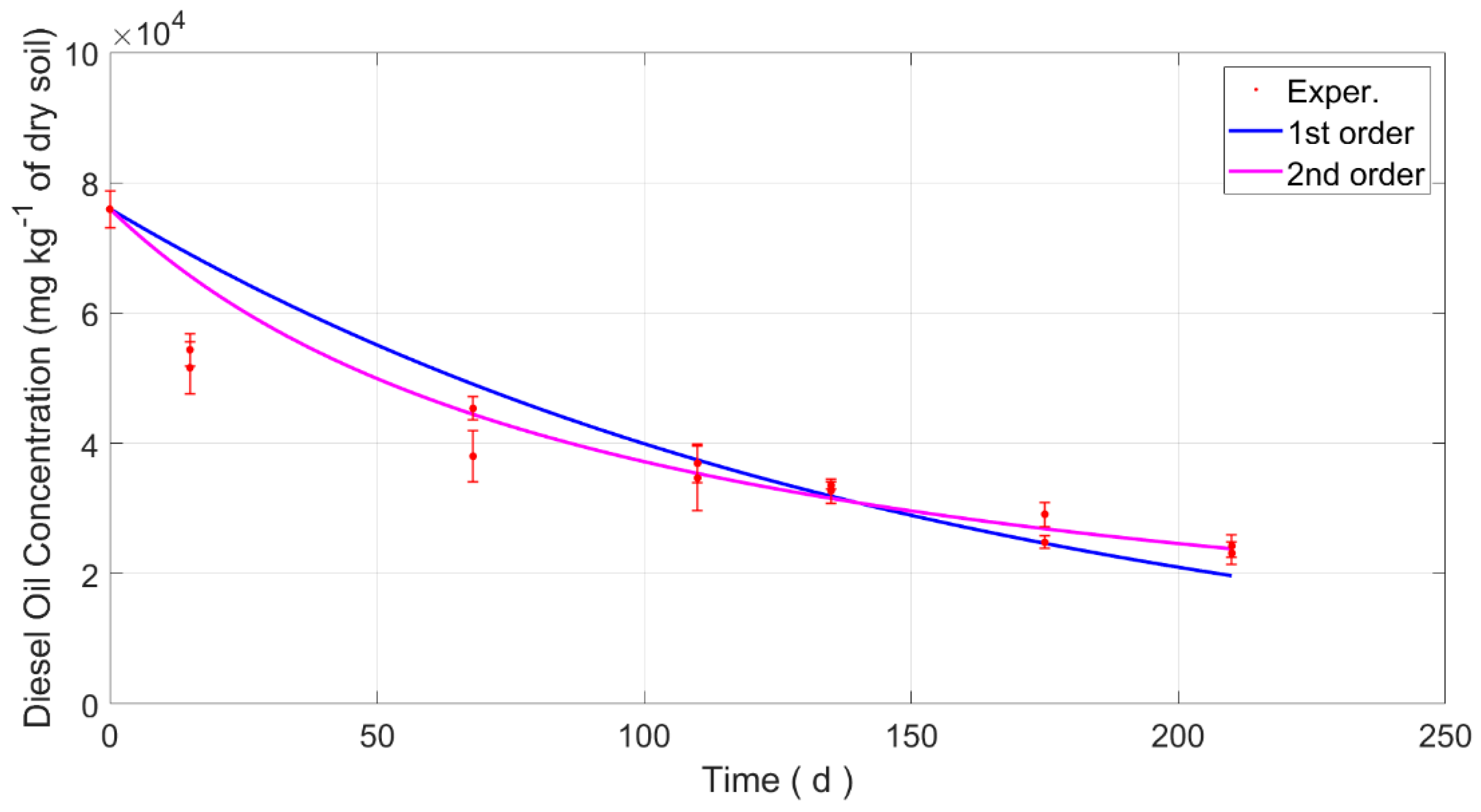
3.4. Kinetic Modeling
3.4.1. First-Order Reaction Rate
The data of residual diesel oil concentration were used to model the process kinetics. As discussed in paragraph 2.6.1, the most widely adopted model is the first-order one.
Looking at the data presented in Figure 5 and as discussed in paragraph 3.3, the diesel oil removal process was not influenced by the presence of glucose; therefore, the results obtained for BIOS and BIOS-G were modeled together. Figure 9 shows these data and the fitting line describing the first-order kinetics, stressed to have C0 = 75926 mg kg−1 of soil. The fitting was performed with the least-square method with uncertain data.
This line has an equation equal to:
C(t) = 75926 exp (−0.0064 t), with R2 = 0.79.
The reaction rate constant was equal to 0.0064 day−1. Using Equation (4), the half-life time t1/2 was calculated: t1/2 = 108 days.
As is evident from Figure 9, the model did not properly fit the experimental data in the first phase of biodegradation (t = 15 and 68 days); for later times, the fitting became adequate. Longer runs could support this reliability, even if it must be noted that for real-scale biodegradation, the processing duration influences the treatment costs, and shorter times are preferable.
3.4.2. Second-Order Reaction Rate
The line modeling the second-order reaction rate is also shown in Figure 9. As for the first-order model, the data fitting was stressed to obtain concentration C = 75926 mg kg−1 of soil at t = 0; as in the previous case, the fitting was performed by the least-square method with uncertain data.
The interpolating equation is 1/C(t) = 1.316 × 10⁻⁵ + 1.373 × 10⁻⁷ × t, and the value of the correlation coefficient is R2 = 0.93. The coefficient was higher than the first-order one, showing that this model seems more suitable to fit the experimental data. Assuming the fitting parameters, the calculation of the half-life time with equation (7) gave t1/2 = 96 days.
3.5. Geophysical Features for Future Monitoring and Preliminary Measurements
A preliminary test to check the behavior of the relative dielectric permittivity and the temperature is shown in Figure 10. The measurements were collected in a sample of the tested system, i.e., sandy soil, partially saturated with water, diesel oil, and gas. A Water Content Reflectometer (WCR) probe was adopted to measure the dielectric permittivity and the sample temperature. We observed a slight increase in the dielectric permittivity when the temperature increased and vice versa.
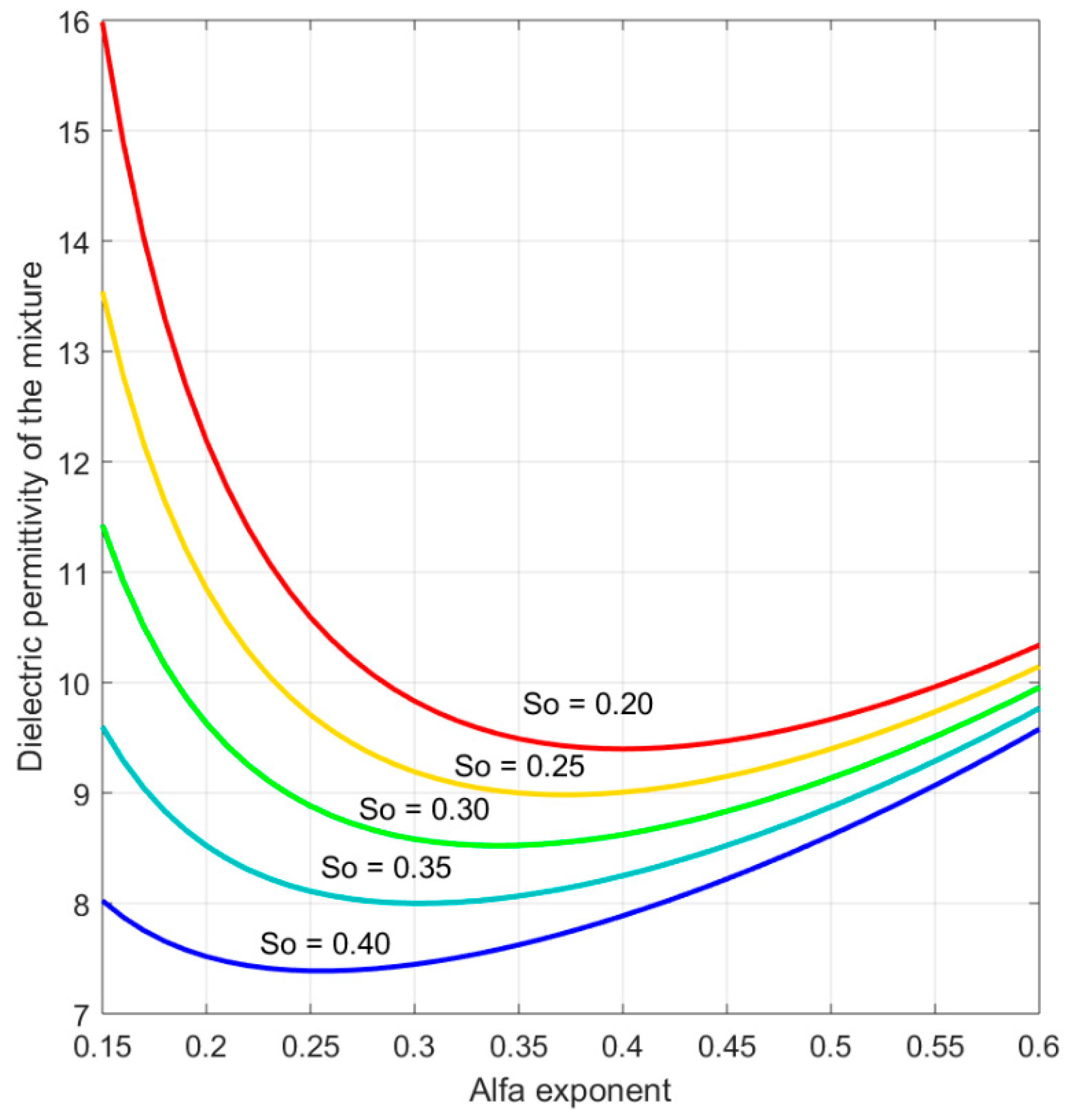
We applied formula (8) to model the behavior of dielectric permittivity of the same mixture of sandy soil, partially saturated with water, oil and gas. The results of the modeling are depicted in Figure 11. The simulation considered a decrease in oil saturation from 0.4 to 0.2, due to the combined effect of evaporation, adsorption and degradation. We assumed that the diesel oil was displaced by gas during the degradation. We plotted the trend of the α-exponent for values of α-exponent in the range 0.2–0.6.
The preliminary measurements showed that the best α-coefficient to match the experimental result is close to being 0.4, considering the uncertainty because of the probe and all the measurements’ inaccuracies.
4. Discussion
Here, we discuss the main findings in terms of biological, kinetic, and geophysical issues. As a biological strategy, biostimulation was adopted, exploiting indigenous microorganisms. The results showed that the overall removal efficiency could be high in a time compatible with common bioremediation treatments, that is to say around 50% in about four months. As a whole, the contribution was the synergic result due to biological and physical removal. Particularly, the abiotic system showed an evident removal of LR species, around 57% of the initial content. Probably, some part of these compounds evaporated and/or was adsorbed; this effect occurred very rapidly. A similar result was obtained by Chen et al. [31]. They studied the bioremediation effect on Total Petroleum Hydrocarbons (TPHs) with biostimulation tests and documented a reduction of TPH mass in the order of 80%, basically due to the removal of aliphatic compounds. A different kind of soil (clay loam soil) was used, and this could be a relevant issue if comparing with our results in sandy soil. Ani and Ochin [32] studied the use of wastes, such as goat manure and palm oil mill effluent, as additional nutrients for the bioremediation of soils polluted with TPHs. Their findings showed the positive effect of these additions when the soil is poor. Therefore, future studies are required to evaluate the effect of soil composition and possible nutrients on the reliability of biostimulation and soil degradation.
The biological contribution can be useful to predict the performance of similar systems, exploiting the indigenous microorganism and enhancing the growth of bacteria populations. The overall effects of the environment can be evaluated in terms of evaporation and soil adsorption.
The sum of these two terms, the biological and the environmental, can estimate the amount of removable pollutant.
The results of the biostimulated microcosms showed that glucose addition did not improve the removal efficiency, and this is a positive issue in terms of real-scale application.
The analysis of the residual diesel oil species showed that, as expected, the simple molecules were removed at a great extent in a short time (15 days), with the synergic contribution of soil and biological process. For the other species, slow removal was shown, completely due to the microbial activity.
In terms of kinetics, the first-order reaction rate was applied with good success to predict the overall amount of removed pollution. This was previously ascertained by other researchers, as shown in paragraph 2.6. Recently, Ortega et al. [33] showed the opportunity to simulate and predict the diesel oil removal from polluted soils by a first-order kinetic modeling able to consider the addition of soil amendments.
In our study, the second order of the reaction rate was also adopted, and it provided a better data fitting with a correlation coefficient equal to 0.93.
The biodegradation results were used to study their impact on an optimal design of future geophysical monitoring. We analyzed the impact on the design of geophysical experiments, both at the laboratory scale and at the field scale. Particularly, if a second order of kinetic is suitable for estimating the behavior of degradation versus time, the time-lapse geophysical experiments must be designed in order to sample with a higher repetition rate the first stage of the degradation, while a first order of kinetic asks for a more regular sampling of the time-lapse experiments.
We focused on the main environmental factors that affect the reliability of laboratory and in-field geophysical monitoring; particularly, we pointed out how the dielectric permittivity depends on the temperature. The monitoring of the temperature is therefore necessary in order to compensate the data for the temperature drift. Particularly, we observed a gradient of dT/dε = 0.1 °C F−1 m, which agrees with similar trends observed in previous works [34]. We did not discuss the temperature effect on the electrical conductivity; this was well documented by several authors [17,34].
We simulated the expected behavior of the dielectric permittivity according to the change in diesel oil saturation, by performing a sensitive analysis (Figure 11). The model reliability had to be checked for every experiment; especially, the optimum value of the α-exponent had to be calibrated. We pointed out that the most favorable condition was yielded when the α-exponent was lower than 0.3, because a higher sensitivity of the dielectric permittivity to the variations of the diesel content was observed. For instance, when α is equal to 0.25, an increase in the dielectric permittivity from 7.5 up to 10.5 is predicted; this is equivalent to a variation of more than 40%. Otherwise, if the α-exponent is equal to 0.5, the simulation predicts an increase in the dielectric permittivity of only about 20%.
According to our sensitivity analysis, the model seemed to be able to predict the degradation rate starting from the geophysical measurements, even if with some uncertainty due to the accuracy of geophysical parameter measurements and reliability of the model. The removal of contaminant inside soil pores produced an increment of soil dielectric permittivity. Therefore, it was directly related to diesel oil reduction, since the contaminant was replaced by the displacing fluid. As also pointed out by Comegna et al. [25], the amount of contaminant in soil can be inferred if the total volume of pore fluid is known in advance.
At this stage of the research, the physical properties of the system are mainly related to the physical and electro-magnetic behaviors of solid media and the chemical and electrical characteristics of fluids. We are not yet considering the interactions between the media, the fluids, and microbes and their metabolic processes. New tests and more detailed analysis are requested in order to understand the geophysical sensitivity of the electromagnetic devices to microbial effects. Particularly, we need to explore how microbial processes could affect the propagation and attenuation terms of the dielectrical permittivity: This could occur at the scale of the cell surface, as suggested by Atenkawa and Slater [35].
Electromagnetic devices, such as WCR and TDR, combine measures of the real part of dielectrical permittivity, which is related to the propagation of the electromagnetic signal, and conductivity, which refers to the attenuation: This integration offers a great opportunity to not only monitor the degradation effects, but also to analyze the microbial activity at the laboratory scale. A good correlation between the presence of hydrocarbon contamination and a substantial increase in electrical conductivity, caused by microbiological activities, was reported in previous studies [36]. Moreover, the long-term degradation of hydrocarbons (in the field) determines a marked attenuation of the electromagnetic signal [37]: In such a context, the monitoring of electrical conductivity, combined with the propagation term (the real part of the dielectrical permittivity), takes on an important role in assessing microbial activity.
This study revealed some findings that are useful for the future application of bioremediation to remove diesel oil from polluted soil, and for planning a strategy for monitoring degradation effects by using a geophysical approach.
Author Contributions
Conceptualization, F.B. and A.G.; methodology, F.B.; software, F.C. and A.G.; validation, F.C.; formal analysis, A.G.; investigation, F.B.; resources, F.B.; data curation, A.C.; writing—original draft preparation, F.C. and A.G.; writing—review and editing, F.C. and A.G.; visualization, F.B.; supervision, F.C.; project administration, F.C.; funding acquisition, F.C.
Funding
This research was funded by the project “GEOPHYSICAL METHODS TO MONITOR SOIL BIOREMEDIATION”, funded by the Italian Ministry of Foreign Affairs and International Cooperation in the frame of the Executive Programme of Scientific and Technological Cooperation between the Republic of India and the Italian Republic for the years 2017–2019—SIGNIFICANT RESEARCH.
Conflicts of Interest
The authors declare no conflict of interest.
References
- Kalantari, R.R.; Mohseni-Bandpi, A.; Esrafili, A.; Nasseri, S.; Ashmagh, F.R.; Jorfi, S.; Ja’fari, M. Effectiveness of biostimulation through nutrient content on the bioremediation of phenanthrene contaminated soil. J. Environ. Health Sci. Eng. 2014, 12, 143. [Google Scholar] [CrossRef]
- Simpanen, S.; Dahli, M.; Gerlach, M.; Mikkonen, A.; Malk, V.; Mikola, J.; Romantschuk, M. Biostimulation proved to be the most efficient method in the comparison of in situ soil remediation treatments after a simulated oil spill accident. Environ. Sci. Pollut. Res. 2016, 23, 25024–25038. [Google Scholar] [CrossRef] [PubMed] [Green Version]
- Poi, G.; Aburto-Medina, A.; Mok, P.C.; Ball, A.S.; Shahsavari, E. Large scale bioaugmentation of soil contaminated with petroleum hydrocarbons using a mixed microbial consortium. Ecol. Eng. 2017, 102, 64–71. [Google Scholar] [CrossRef]
- Fan, M.Y.; Xie, R.-J.; Qin, G. Bioremediation of petroleum-contaminated soil by a combined system of biostimulation–bioaugmentation with yeast. Environ. Technol. 2014, 35, 391–399. [Google Scholar] [CrossRef] [PubMed]
- Wu, M.; Dick, W.A.; Li, W.; Wang, X.; Yang, Q.; Wang, T.; Xu, L.; Zhang, M.; Chen, L. Bioaugmentation and biostimulation of hydrocarbon degradation and the microbial community in a petroleum-contaminated soil. Int. Biodeterior. Biodegrad. 2016, 107, 158–164. [Google Scholar] [CrossRef]
- Guarino, C.; Spada, V.; Sciarrillo, R. Assessment of three approaches of bioremediation (Natural attenuation, Landfarming and Bioagumentation-Assistited Landfarming) for a petroleum hydrocarbons contaminated soil. Chemosphere 2017, 170, 10–16. [Google Scholar] [CrossRef] [PubMed]
- Liu, X.; Selonen, V.; Steffen, K.; Surakka, M.; Rantalainen, A.-L.; Romantschuk, M.; Sinkkonen, A. Meat and bone meal as a novel biostimulation agent in hydrocarbon contaminated soils. Chemosphere 2019, 225, 574–578. [Google Scholar] [CrossRef]
- Safdari, M.-S.; Kariminia, H.-R.; Rahmati, M.; Fazlollahi, F.; Polasko, A.; Mahendra, S.; Wilding, W.V.; Fletcher, T.H. Development of bioreactors for comparative study of natural attenuation, biostimulation, and bioaugmentation of petroleum-hydrocarbon contaminated soil. J. Hazard. Mater. 2018, 342, 270–278. [Google Scholar] [CrossRef]
- Wu, M.; Li, W.; Dick, W.A.; Ye, X.; Chen, K.; Kost, D.; Chen, L. Bioremediation of hydrocarbon degradation in a petroleum-contaminated soil and microbial population and activity determination. Chemosphere 2017, 169, 124–130. [Google Scholar] [CrossRef]
- Lopes Julio, A.D.; Rocha Fernandes, R.d.C.; Dutra Costa, M.; Lima Neves, J.C.; Montes Rodrigues, E.; Rogerio Totola, M. A new biostimulation approach based on the concept of remaining P for soil bioremediation. J. Environ. Manag. 2018, 207, 417–422. [Google Scholar] [CrossRef]
- Polyak, Y.M.; Bakina, L.G.; Chugunova, M.V.; Mayachkina, N.; Gerasimov, A.; Bure, V.M. Effect of remediation strategies on biological activity of oil-contaminated soil—A field study. Int. Biodeterior. Biodegrad. 2018, 126, 57–68. [Google Scholar] [CrossRef]
- Casale, A.; Bosco, F.; Chiampo, F.; Franco, D.; Ruffino, B.; Godio, A. Soil microcosm set up for a bioremediation study. Int. J. Appl. Sci. Environ. Eng. 2018, 1, 277–280. [Google Scholar]
- Bosco, F.; Casale, A.; Mazzarino, I.; Godio, A.; Ruffino, B.; Mollea, C.; Chiampo, F. Microcosm evaluation of bioaugmentation and biostimulation efficacy on diesel-contaminated soil. J. Chem. Technol. Biotechnol. 2019. [Google Scholar] [CrossRef]
- Arato, A.; Weher, M.; Bíró, B.; Godio, A. Integration of geophysical, geochemical and microbiological data for a comprehensive small-scale characterization of an aged LNAPL-contaminated site. Environ. Sci. Pollut. Res. 2014, 1, 8948–8963. [Google Scholar] [CrossRef]
- Koroma, S.; Arato, A.; Godio, A. Analyzing geophysical signature of a hydrocarbon-contaminated soil using geoelectrical surveys. Environ. Earth Sci. 2015, 74, 2937–2948. [Google Scholar] [CrossRef]
- Atekwana, E.A.; Werkema, D.D.; Atekwana, E.A. Biogeophysics: The effects of microbial processes on geophysical properties of the shallow subsurface. Appl. Hydrogeophys. 2006, 71, 161–193. [Google Scholar] [CrossRef]
- Or, D.; Wraith, J.M. Temperature effects on soil bulk dielectric permittivity measured by time domain reflectometry: A physical model. Water Resour. Res. 1999, 35, 371–383. [Google Scholar] [CrossRef]
- Lazebnik, M.; Converse, M.; Booske, J.H.; Hagness, S.C. Ultra-wideband Temperature-Dependent Dielectric Properties of Animal Liver Tissue in the Microwave Frequency Range. Phys. Med. Biol. 2006, 51, 1941–1955. [Google Scholar] [CrossRef]
- Godio, A. Open ended-coaxial Cable Measurements of Saturated Sandy Soils. Am. J. Environ. Sci. 2007, 3, 175–182. [Google Scholar] [CrossRef]
- Endres, A.L.; Redman, D.J. Modeling the electrical properties of porous rocks and soils containing immiscible contaminants. J. Environ. Eng. Geophys. 2009, 105–112. [Google Scholar] [CrossRef]
- Carcione, J.M.; Seriani, G. An electromagnetic modelling tool for the detection of hydrocarbons in the subsoil. Geophys. Prospect. 2000, 48, 231–256. [Google Scholar] [CrossRef]
- Sen, P.N.; Scala, C.; Cohen, M.H. A self-similar model for sedimentary rocks with applications to the dielectric constant of fused glass beads. Geophysics 1981, 46, 781–795. [Google Scholar] [CrossRef]
- Feng, S.; Sen, P.N. Geometrical model of conductive and dielectric properties of partially saturated rocks. J. Appl. Phys. 1985, 58, 3236–3243. [Google Scholar] [CrossRef]
- Knight, R.; Endres, A. A new concept in modeling the dielectric response of sandstones: Defining a wetted rock and bulk water system. Geophysics 1990, 55, 586–594. [Google Scholar] [CrossRef] [Green Version]
- Comegna, A.; Coppola, A.; Dragonetti, G.; Sommella, A. Dielectric response of a variable saturated soil contaminated by Non-Aqueous Phase Liquids (NAPLs). Procedia Environ. Sci. 2013, 19, 701–710. [Google Scholar] [CrossRef]
- Adesodun, J.K.; Mbagwu, J.S.C. Biodegradation of waste-lubricating petroleum oil in a tropical alfisol as mediated by animal droppings. Bioresour. Technol. 2008, 99, 5659–5665. [Google Scholar] [CrossRef]
- Agarry, S.E.; Aremu, M.O.; Aworanti, A. Kinetic Modelling and Half-Life Study on Bioremediation of Soil Co-Contaminated with Lubricating Motor Oil and Lead Using Different Bioremediation Strategies. Soil Sediment Contam. Int. J. 2013, 22, 800–816. [Google Scholar] [CrossRef]
- Komilis, D.P.; Vrohidou, A.E.K.; Voudrias, E.A. Kinetics of aerobic bioremediation of a diesel-contaminated sandy soil: Effect of nitrogen addition. Water Air Soil Pollut. 2010, 208, 193–208. [Google Scholar] [CrossRef]
- Nwankwegu, A.S.; Onwosi, C.O. Bioremediation of gasoline contaminated agricultural soil by bioaugmentation. Environ. Technol. Innov. 2017, 7, 1–11. [Google Scholar] [CrossRef]
- Sarkar, D.; Ferguson, M.; Datta, R.; Birnbaum, S. Bioremediation of petroleum hydrocarbons in contaminated soils: Comparison of biosolids addition, carbon supplementation, and monitored natural attenuation. Environ. Pollut. 2005, 136, 187–195. [Google Scholar] [CrossRef]
- Chen, F.; Li, X.; Zhu, Q.; Ma, J.; Hou, H.; Zhang, S. Bioremediation of petroleum-contaminated soil enhanced by aged refuse. Chemosphere 2019, 222, 98–105. [Google Scholar] [CrossRef]
- Ani, K.A.; Ochin, E. Response surface optimization and effects of agricultural wastes on total petroleum hydrocarbon degradation. Beni-Suef Univ. J. Basic Appl. Sci. 2018, 7, 564–574. [Google Scholar] [CrossRef]
- Ortega, M.F.; García-Martínez, M.-J.; Bolonio, D.; Canoira, L.; Llamas, J.F. Weighted linear models for simulation and prediction of biodegradation in diesel polluted soils. Sci. Total Environ. 2019, 686, 580–589. [Google Scholar] [CrossRef]
- Seyfried, S.S.; Grant, L.E. Temperature Effects on Soil Dielectric Properties Measured at 50 MHz. Vadose Zone J. 2007, 6, 759–765. [Google Scholar] [CrossRef] [Green Version]
- Atekwana, E.A.; Slater, L. Biogeophysics: A new frontier in Earth science research. Rev. Geophys. 2009, 47, RG4004. [Google Scholar] [CrossRef]
- Cassiani, G.; Binley, A.; Kemna, A.; Wehrer, M.; Flores Orozco, A.; Deiana, R.; Boaga, J.; Rossi, M.; Dietrich, P.; Werban, U.; et al. Noninvasive characterization of the Trecate (Italy) crude-oil contaminated site: Links between contamination and geophysical signals. Environ. Sci. Pollut. Res. 2014, 21, 8914–8931. [Google Scholar] [CrossRef]
- Godio, A.; Arato, A.; Stocco, S. Geophysical characterization of a non aqueous-phase liquid-contaminated site. Environ. Geosci. 2010, 17, 141–162. [Google Scholar] [CrossRef]
Figure 1.
Cumulative amount of CO2 production due to microbial respiration (A = abiotic microcosm; BIOS = biostimulated microcosm; BIOS-G = biostimulated microcosm and glucose addition; C = control microcosm).
Figure 1.
Cumulative amount of CO2 production due to microbial respiration (A = abiotic microcosm; BIOS = biostimulated microcosm; BIOS-G = biostimulated microcosm and glucose addition; C = control microcosm).

Figure 2.
Cumulative amount of CO2 production of a biotic microcosm (natural soil).

Figure 3.
Difference in CO2 production due to glucose addition.

Figure 4.
Microbial count at different times in the experimental tests’ respiration (BIOS = biostimulated microcosm; BIOS-G = biostimulated microcosm and glucose addition; C = control microcosm).
Figure 4.
Microbial count at different times in the experimental tests’ respiration (BIOS = biostimulated microcosm; BIOS-G = biostimulated microcosm and glucose addition; C = control microcosm).

Figure 5.
Residual diesel oil concentration in microcosms’ respiration (A = abiotic microcosm; BIOS = biostimulated microcosm; BIOS-G = biostimulated microcosm and glucose addition).
Figure 5.
Residual diesel oil concentration in microcosms’ respiration (A = abiotic microcosm; BIOS = biostimulated microcosm; BIOS-G = biostimulated microcosm and glucose addition).

Figure 6.
Change in residual diesel oil composition during the process for the abiotic microcosm.

Figure 7.
Change in residual diesel oil composition during the process for the BIOS microcosm.

Figure 8.
Change in residual diesel oil composition during the process for the BIOS-G microcosm.

Figure 9.
Kinetic modelling for the BIOS and BIOS-G microcosms.

Figure 10.
Relative dielectric permittivity (red) and temperature (black) measured in a mixture of sandy grain, diesel oil, water and gas (measurements performed with a Water Content Probe). The measures refer to a time-window of 24 h.
Figure 10.
Relative dielectric permittivity (red) and temperature (black) measured in a mixture of sandy grain, diesel oil, water and gas (measurements performed with a Water Content Probe). The measures refer to a time-window of 24 h.

Figure 11.
Effect of α-exponent of the CRIM formula on relative dielectric permittivity at different diesel oil contents (So), considering a relative water content of 0.4.
Figure 11.
Effect of α-exponent of the CRIM formula on relative dielectric permittivity at different diesel oil contents (So), considering a relative water content of 0.4.


Table 1.
Chemical and geophysical soil properties.
| Chemical Parameter | Value |
| pH | 7.32 ± 0.04 |
| Soluble bicarbonate (mg kg−1 of dry soil) | 66.9 ± 10.8 |
| Soluble chlorides (mg kg−1 of dry soil) | 26.2 ± 0.3 |
| Soluble sulphates (mg kg−1 of dry soil) | 211 ± 3 |
| Ammonia (mg kg−1 of dry soil) | 2.18 ± 0.11 |
| Nitrates (mg kg−1 of dry soil) | 68.0 ± 0.4 |
| Geophysical Parameter | Value |
| Porosity (% volume) | 40–42 |
| Density (kg m−3) | 2700 |
| Dielectric permittivity for dry soil | 2.5–3 |
| Dielectric permittivity for saturated soil | 25–30 |
Table 2.
Reference values of relative dielectric permittivity for the materials adopted in the sensitivity analysis.
Table 2.
Reference values of relative dielectric permittivity for the materials adopted in the sensitivity analysis.
| Phase | Relative Dielectric Permittivity | Method |
|---|---|---|
| Solid (grains) | 3.2 +/− 0.2 | Estimated according to Complex Refractive Index Model (CRIM) formula on saturated specimen (Time Domain Reflectometry (TDR) probe) [24] |
| Water | 78.5 +/− 0.2 (at 25 °C) | Measured with TDR probe [25] |
| Diesel oil | 2.2 +/− 0.1 | Measured with Open-Ended-Coaxial cable [19] |
© 2019 by the authors. Licensee MDPI, Basel, Switzerland. This article is an open access article distributed under the terms and conditions of the Creative Commons Attribution (CC BY) license (http://creativecommons.org/licenses/by/4.0/).
Share and Cite
MDPI and ACS Style
Bosco, F.; Casale, A.; Chiampo, F.; Godio, A. Removal of Diesel Oil in Soil Microcosms and Implication for Geophysical Monitoring. Water 2019, 11, 1661. https://doi.org/10.3390/w11081661
AMA Style
Bosco F, Casale A, Chiampo F, Godio A. Removal of Diesel Oil in Soil Microcosms and Implication for Geophysical Monitoring. Water. 2019; 11(8):1661. https://doi.org/10.3390/w11081661
Chicago/Turabian StyleBosco, Francesca, Annalisa Casale, Fulvia Chiampo, and Alberto Godio. 2019. "Removal of Diesel Oil in Soil Microcosms and Implication for Geophysical Monitoring" Water 11, no. 8: 1661. https://doi.org/10.3390/w11081661
Note that from the first issue of 2016, this journal uses article numbers instead of page numbers. See further details here.