Assessment of the Physically-Based Hydrus-1D Model for Simulating the Water Fluxes of a Mediterranean Cropping System

Abstract

In a context characterized by a scarcity of water resources and a need for agriculture to cope the increase of food demand, it is of fundamental importance to increase the water use efficiency of cropping systems. This objective can be meet using several currently available software packages simulating water movements in the “soil–plant–atmosphere” continuum (SPAC). The goal of the paper is to discuss and optimize the strategy for implementing an effective simulation framework in order to describe the main soil water fluxes of a typical horticultural cropping system in Southern Italy based on drip-irrigated watermelon cultivation. The Hydrus-1D model was calibrated by optimizing the hydraulic parameters based on the comparison between simulated and measured soil water content values. Next, a sensitivity analysis of the hydraulic parameters of the Mualem–van Genuchten model was carried out. Hydryus-1D determined simulated soil water contents fairly well, with an average root mean square error below 9%. The main fluxes of the SPAC were confined in a restricted soil volume and were therefore well described by the one-dimensional model Hydrus-1D. Water content at saturation and the fitting parameters α and n were the parameters with the highest impact for describing the soil/plant water balance.

1. Introduction

In many regions of the world, scarcity of water resources is one of the most important concerns for agriculture, together with increasing food demand due to increasing population and rapid economic growth. These concerns are exacerbated by the impacts of climate change on crop yield [1], fresh water availability, and soil fertility. In this scenario, above all in environments with high degrees of evapotranspiration, it becomes of fundamental importance to increase the water use efficiency of cropping systems by acting on the optimization of irrigation (method, amount, and timing) and the application of suitable irrigation scheduling for crops cultivated in dry environments, where irrigation is one of the essential agronomical practices to obtain sustainable yields. For these reasons, many software packages, with different complexity levels, are available and are used for simulating water movement in the “soil–plant–atmosphere” continuum and estimating indicators useful for increasing water use efficiency.

Among the available models, the physically-based models ones, i.e., based on numerical solutions of the Richards equation, are increasingly being used to simulate water and solute movement in the vadose zone for a variety of common applications in research and soil/water management (see for example [2,3,4,5,6]).

Hydrus software packages are finite element models for simulating the one- and two- or three-dimensional movement of water, heat, and multiple solutes in variably saturated media, and since their implementation they have been extensively applied in various applications. Hydrus-1D, with related manuals and case studies as examples, can be freely downloaded from the Hydrus website (https://www.pc-progress.com/en/Default.aspx?hydrus-1d) [7].

In the Mediterranean environment of Southern Italy, one of the first applications of Hydrus-1D concerned the simulation of water movement and solute transport in a variably saturated water flow of fine-textured soil subjected to a fluctuating saline groundwater table [8]. Since then, the use of Hydrus has involved the estimation of the water fluxes under several cropping systems differentiated from a spatial and agronomical point of view.

Plastic mulch is an agronomic technology widespread in the world because it allows farmers and engineers: (1) to increase soil temperature, (2) to reduce weed pressure and certain insect pests, (3) to increase the soil moisture, and (4) to improve nutrient use efficiency [9,10,11]. Under cotton cultivation, for example, the effect of plastic mulch on soil water balance under drip irrigation has been examined by Han et al. [9], who revealed a minimal effect on soil water distribution but a real effectiveness on soil water conservation due to a great reduction of soil evaporation.

Hydrus was used also to check out the optimal drip lateral depth under a cropping system of eggplant characterized by large inter-row distance and localized irrigation [12]. Recently, the dynamics of soil water contents and water fluxes in an olive orchard, submitted to two irrigation systems, were assessed by Autovino et al. [2]. The abovementioned studies were based on Hydrus-2D, which simulates two-dimensional water movements, with the assumption of the absence of water pressure head gradient along the plant rows. The use of Hydrus-2D can lead to higher complexity in terms of discretization of the domain and running simulation time when compared to the one-dimensional Hydrus-1D version. However, using physically-based models can be useful for increasing water use efficiency, saving water, and minimizing risks of water percolation and leaching.

In the case of horticultural systems, characterized by wide inter-rows, a one-dimensional domain could be suitable if the infiltration of irrigated water, root absorption, and percolation took place in a confined volume and not on the entire surface of the soil. This condition generally occurs with localized irrigation, which aims to distribute water in a limited volume of soil explored by the roots. However, this condition also depends on soil properties and agronomic management (presence or absence of plastic mulch, tillage, methods of fertilization, etc.), and the optimization of these factors needs to be carefully investigated for specific agro-environments.

Although physically-based models for simulating the one- and two- or three-dimensional movements of water are effective for estimating field-scale water fluxes, they generally require complex model parameterizations and input variables, some of which are not readily available. In order to address the issue of missing soil hydraulic parameters, which is particularly important for regional studies, a common approach is to use pedotransfer functions to convert available soil information, such as texture, bulk density, etc., to soil hydraulic parameters [13]. Hydrus packages make use of the pedotransfer functions (PTFs) based on neural networks [14] to predict van Genuchten’s [15] water retention parameters and the saturated hydraulic conductivity (Ks) by means of textural information, bulk density, and soil water content at a pressure head (h) of −300 and −15,000 cm (i.e., at field capacity and permanent wilting point, respectively).

The aim of this study is to discuss and optimize the strategy regarding the characterization of soil, the impact of its accurate description and the implementation of an effective simulation framework in order to describe the main soil water fluxes of the “soil–plant–atmosphere” continuum for a typical horticultural cropping system based on drip-irrigated watermelon cultivation in Southern Italy.

2. Materials and Methods

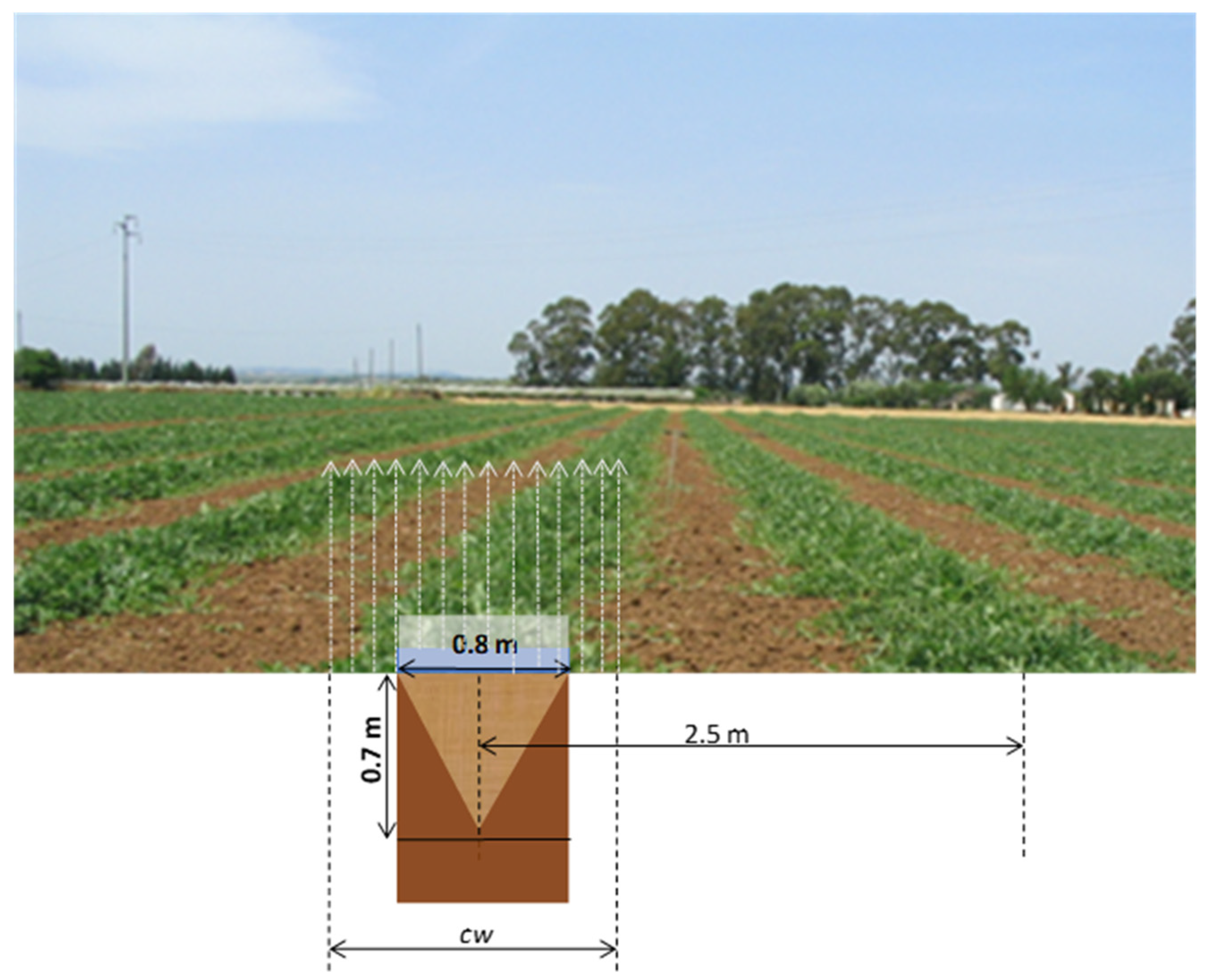
2.1. Experimental Site

In a field of a private farm cultivated with drip-irrigated watermelon (Citrullus lanatus, Thunb) located in Castellaneta (Southern Italy, 40°35′29.01″ N, 16°55′26.18″ E), an automated Time Domain Reflectometry (TDR) system, installed in May 2006, was used to continuously measure soil-moisture content variations on hourly basis (Figure 1). The TDR system included a cable tester (TDR100) interfaced to a data logger (CR10) and multiplexers, a solar panel, and a storage battery (Campbell Scientific, Logan, UT, USA). The waveguides probes consisted of three 15-cm stainless-steel rods. Three probes were inserted in the middle between two plant rows, horizontally from field level and perpendicular to the rows. Another 16 probes were horizontally inserted below the drip lines, and plant rows in four profiles each consisted of four probes inserted at −10, −30, −50, and −70 cm depths. The TDR system was removed in July. Analysis of the waveforms curves was automatically performed by adopting the procedure implemented in CR10 and the volumetric soil water content (SWC) was estimated by the general equation of Topp et al. [16].

Table 1. Physical and chemical of soil characteristics.

Parameter	Unit	First Layer 0–20 cm	Second Layer 20–40 cm
pH		8.23	8.15
Electrical conductivity	dS m−1	0.366	0.4632
Total organic carbon	g kg−1	10.0	9.7
Total nitrogen	g kg−1	0.99	0.99
Sand	%	16.48	16.33
Silt	%	36.10	37.32
Clay	%	47.43	46.35
Dry bulk density	g cm−3	1.27	1.36
Field capacity	cm3 cm−3	0.37	0.38
Permanent wilting point	cm3 cm−3	0.19	0.20

reports the main characteristics for two soil layers (0–20 and 20–40 cm depth). The soil is a clay with a total organic carbon close to the USDA lower normal limit (10 g kg⁻¹). Comparable values of field capacity and permanent wilting point were detected in the soil profile, although it was slightly more compact in the lower layer than in the superficial one (Table 1). A visual inspection of soil profile (1 m depth) during the installation of the TDR probes showed that the soil was quite homogeneous and consequently we extended the hydraulic properties of second layer to all the domain profile up to the considered bottom boundary.

The climate of the area is typically Mediterranean, with mean monthly minimum temperatures of 2.7 °C in the winter and maximum temperature of 27 °C in the summer. The 30-year mean annual precipitation of the area is 638 mm, with more than 60% of the rainfall occurring from October through March (www.ilmeteo.it/portale/medie-climatiche/Castellaneta).

In the field of watermelon, the inter-row distance was of 2.50 m with a plant distance in the row of 0.90 m. Before the transplanting time, a black plastic mulch, 35 cm wide, was placed on the rows in order to reduce the water evaporation losses and to control the weed germination and growth. Below the plastic mulch, a soft drip-line with holes every 30 cm and flow rate (q) of 1.2 l h⁻¹ was placed on each row. The duration (t_i, hour) of each irrigation event was estimated by analysing the daily trend of soil water content (SWC) measured by the shallowest TDR probe (−10 cm) which, throughout the irrigation, indicated a rapid increase of SWC. The irrigation depth (v_i, mm) was estimated, through the following equation:

$$v_i=\frac{t_i{n}_{e}q}{A}$$

(1)

where n_e is the number of the emitters of the drip line (130 m long) equipped with volumetric meter and A is the product of 130 m by 0.8 m, with this last parameter being the width of the area served by the drip hole, visually estimated and constant throughout the crop cycle. Each v_i was verified by the water volume measured by the volumetric meter installed on the drip hole of the monitored row. The irrigation volumes supplied by the farmer were of 3239 m³ ha⁻¹.

During the watermelon cultivation, the following measurements were carried out at a weekly or ten-day scale: gravimetric SWC at two depths using disturbed soil cores; perpendicular variation in shallow SWC through regular measurements between two adjacent rows utilizing the 5-cm “Theta Probes ML2x” transept in the inter-row; and soil bulk density with undisturbed soil cores (5 cm in diameter by 5 cm in height). Regarding the crop growth, every week the canopy width (cw) along the rows was monitored and a ceptometer (LP-80, Decagon Devices, Inc., Pullman, WA, USA) was utilized for measuring the canopy cover index (i).

To estimate reference evapotranspiration, ET₀, close to TDR probes, a standard meteorological station was installed for monitoring hourly air temperature, humidity, global radiation, precipitation and wind speed at a 2-m height. Daily values of ET₀ were determined according to the FAO Penman–Monteith equation [17].

Because of the plastic mulch placed on the row, the soil evaporation was considered equal to 0 and the adjusted potential daily plant transpiration ($T_P^{\prime }$) was estimated by:

$$\begin{gathered} T_P=E{T}_{0}i, \\ {T}_P^{\prime }=c{T}_P \end{gathered}$$

(2)

where c (>1) is the ratio between cw, the measured width of the transpirating canopy, and the reference width (0.8 m) of the considered soil domain in which the watermelon roots were developed and concentrated (Figure 1). The adjustment of the potential transpiration is necessary to be able to use a one-dimensional model for crops with root apparatus concentrated below a soil surface smaller than that of the canopy and in a volume of soil wetted by drip irrigation.

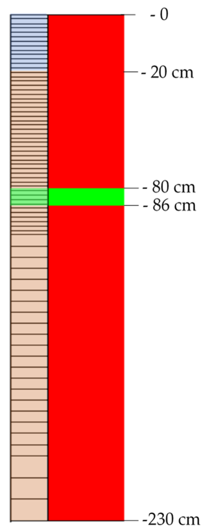
2.2. Modelling Approach

The Hydrus-1D software (version 4.17) [18] was used to simulate one-dimensional vertical isothermal variably-saturated flow at the experimental site and below the drip line and plastic mulch, considering the soil uniformly irrigated and explored by the roots.

Simulations were performed from 30 May to 25 July 2006. The one-dimensional flow domain extended to a depth of 2.3 m, and was divided into two separate soil layers, from 0 to −20 cm and from −20 to −230 cm, comprising a total of 74 finite elements. A finer discretization was used near the soil surface to accommodate relatively steep gradients in the pressure head. Four observational nodes were seated in the soil profile in correspondence with the TDR probe at depths of −10, −30, −50, and −70 cm. As a soil surface boundary condition, we used a system-dependent atmospheric condition in accordance with the approach of Feddes [19] and Šimůnek et al. [18]. The time variable conditions of top boundary were defined at daily scale by irrigation depth ($v_i$, Equation (1)) and adjusted potential transpiration ($T_P^{\prime },$ Equation (2)). At the bottom boundary a “free drainage” condition was adopted. It is determined by an unit vertical hydraulic gradient implemented in Hydrus-1D as a form of a variable flux boundary condition, suitable for cases where the water table is very deep and does not affect the crop/soil water balance. The root water uptake stress response function of Feddes [19] was used optimizing the related parameters in a preliminary calibration phase. The initial conditions were considered as the hydraulic potential for a profile in equilibrium after the heavy irrigations were carried out in the area during the first phase of melon cultivation.

The daily output variables simulated by Hydrus-1D and utilized in this study were: (1) transient SWC at observational points, (2) water potential in the soil explored by the roots, (3) cumulated actual soil water uptake, (4) infiltration, and (5) deep percolation.

The soil hydraulic functions were described according to van Genuchten [15]:

$$S_e=\frac{\theta -{\theta }_r}{{\theta }_s-{\theta }_r}={\left[1+{\left(\alpha h\right)}^n\right]}^{-m}$$

(3)

$$K=K_s{S}_e{}^{0.5}{\left[1-{\left(1-S_e{}^{1/m}\right)}^m\right]}^2$$

(4)

where S_e is the relative saturation, θ_s and θ_r are the saturated and residual water content (m³ m⁻³), h is the soil water pressure head (cm), α (cm⁻¹) and n are fitting parameters m = 1 − (1/n), and K_s is the saturated hydraulic conductivity (cm d⁻¹).

In order to calibrate Hydrus-1D, four sets of hydraulic parameters (C1 to C4) obtained by applying the pedotransfer function of Rosetta [14] were considered. In particular, in C1 the parameters were estimated utilizing as independent variables the percentages of clay, silt, and sand of the two soil layers considered (0/–20 cm, −21/–230 cm). C2 also takes into account the measured bulk density, whereas the measured soil water contents at soil water potential of −300 cm and −15,000 cm were included as independent variables for C3 and C4, respectively. In this investigation, we considered as a reference a fifth set of parameters (C5) obtained by the Wind evaporation method [20] and the Unit hydraulic gradient (Uhg) method [21,22]. Thus, the four considered sets (C1–C4) were compared for validation purposes with the reference parameters (C5). In details, the Wind and Uhg methods allowed us to obtain an accurate soil hydraulic characterization, namely to estimate the water retention curve and the hydraulic conductivity function of investigated soil. For this purpose, two soil cores (0.075 m in height by 0.085 m in diameter) were subjected, in sequence, to a 1D unsaturated infiltration process and to a transient stage of evaporation to estimate the hydraulic properties of the soil in the 0–10 and 11–20 cm layers. Practically, during the transient of evaporation, applied methods provides θ-h-K values which need to be interpolated to obtain the water retention curve (θ-h) and hydraulic conductivity (K-h) functions. As a consequence, hydraulic functions were simultaneously parameterized by applying the Metronia code [23]. Details about applied methodologies, i.e., Unit hydraulic gradient and Wind evaporation methods, can be found in Bagarello et al. [22,24], respectively.

The

Table 2. Van Genuchten parameters of the five approaches.

Approach	Layer (cm)	θr	θs	α	n	Ks
C1	0–20	0.0911	0.4554	0.0204	1.2546	11.36
	21–230	0.0910	0.4577	0.0193	1.2667	10.76
C2	0–20	0.0992	0.5015	0.0185	1.3257	24.74
	21–230	0.0955	0.4738	0.0172	1.325	15.75
C3	0–20	0.0901	0.4986	0.021	1.2525	37.84
	21–230	0.0890	0.4714	0.0177	1.2536	20.10
C4	0–20	0.0722	0.4916	0.0076	1.378	30.75
	21–230	0.0706	0.4694	0.0061	1.392	18.05
C5	0–230	0.1784	0.5049	0.0522	1.324	116.41

reports the parameters of the 5 approaches. For C5 a single layer was considered because lab experiments provided similar results between soil layers.

An accurate analysis of SWC profiles and moisture temporal fluctuations, following the infiltration and drying–redistribution processes, irrigation/rainfall events, and crop evapotranspiration, allowed us to obtain useful information on the root spatial distribution, both in terms of root density and maximum root depth reached during the crop growth cycle [25]. The first step of this methodology was to identify in the transient of θ(z,t) a suitable time frame between two irrigations/rain events in which the soil water reservoir has been depleted by roots. Figure 2 shows the SWC soil profiles of the selected time frame from 5 July to 13 July. The root water uptakes (RWU_z, m³ m⁻³), for each TDR probe location, were determined by calculating the differences in SWC between the irrigation of 5 July, and 13 July, the day prior to the next irrigation. RWUz values were scaled by total water uptake calculated on a daily basis, ρ(z,t) (m³ m⁻³ d⁻¹), and the normalized uptake volume ρ’(z,t), under the hypothesis that it is a useful indicator of root density in agreement with Coelho and Or [25], was calculated as:

$$RWUz\equiv {\rho }^{\prime }\left(z,t\right)=\frac{\rho \left(z,t\right)}{{{\displaystyle \sum }}_z\rho \left(z,t\right)}$$

(5)

Figure 2 shows ρ’(z,t) as a function of the relative depth, z/z_r, where z_r was 70 cm. The watermelon root apparatus deepened in the first 70 cm of the soil profile, with most of it (about 70%) developed in the first 50 cm. These two parameters were used to define the root sub-model available in Hydrus-1D.

2.3. Hydraulic Conductivity Measurements

Single ring infiltration measurements of the Beerkan type [26,27] were carried out on a clay soil at the experimental farm of CREA-AA, Foggia (41°27′03″ N, 15°30′06″ E). This fine textured soil was chosen with the aim (1) to apply several models for single ring infiltration data, to estimate the saturated hydraulic conductivity of the soil, Ks, and (2) to use these Ks values as an alternative to synthetically generated data to evaluate the impact of Ks on soil hydraulic parameter optimization.

Specifically, a wide range of Ks values was obtained on undisturbed and tilled plots between December and June (five sampling dates), during the crop season of durum wheat; this allowed us to consider a relatively wide variability of the physical and hydraulic properties of the soil. For a given date or plot, 5–12 infiltration experiments were carried out, and a total of 78 cumulative infiltrations were determined. The single-ring infiltration model of Stewart and Abou Najm [28] and the SSBI method (steady version of the simplified method based on a Beerkan infiltration run) proposed by Bagarello et al. [29] were used to estimate Ks from Beerkan infiltration experiments. More specifically, we considered nine different calculation approaches corresponding to scenarios vi-xiv described in detail by Di Prima et al. [5]. Briefly, those calculation approaches differed by: (1) the way they constrained the macroscopic capillary length, (2) the use of transient or steady-state infiltration data, and (3) the fitting methods applied to transient data. The obtained Ks data set ranged more than two orders of magnitude between min and max Ks values.

2.4. Parametrization Evaluation

Statistical indicators were used to compare the performance of Hydrus-1D regarding the modelling of SWC and TDR observations at different depths. For this purpose, we applied the IRENE software, a tool designed to carry out statistical analysis for use in model evaluation [30]. Specifically, the five approaches for estimating the van Genuchten parameters were compared on the basis of 24 statistical indicators. The five approaches (C1 to C5) were ranked according to the best value reached by each statistical indicator by attributing a weight of 5 and 1 for the best and worst performance, respectively.

The ranking index for each approach was calculated by averaging the 24 relative weights. In this paper only 11 statistical indicator will be reported: absolute and relative root mean squared error [31], modeling efficiency [32], index of agreement [33], coefficient of determination and of residual mass [34], mean absolute error [35], regression coefficient with slope and intercept, and standard error. The aforementioned references are reported in the documentation included in the software package of IRENE [30].

3. Results

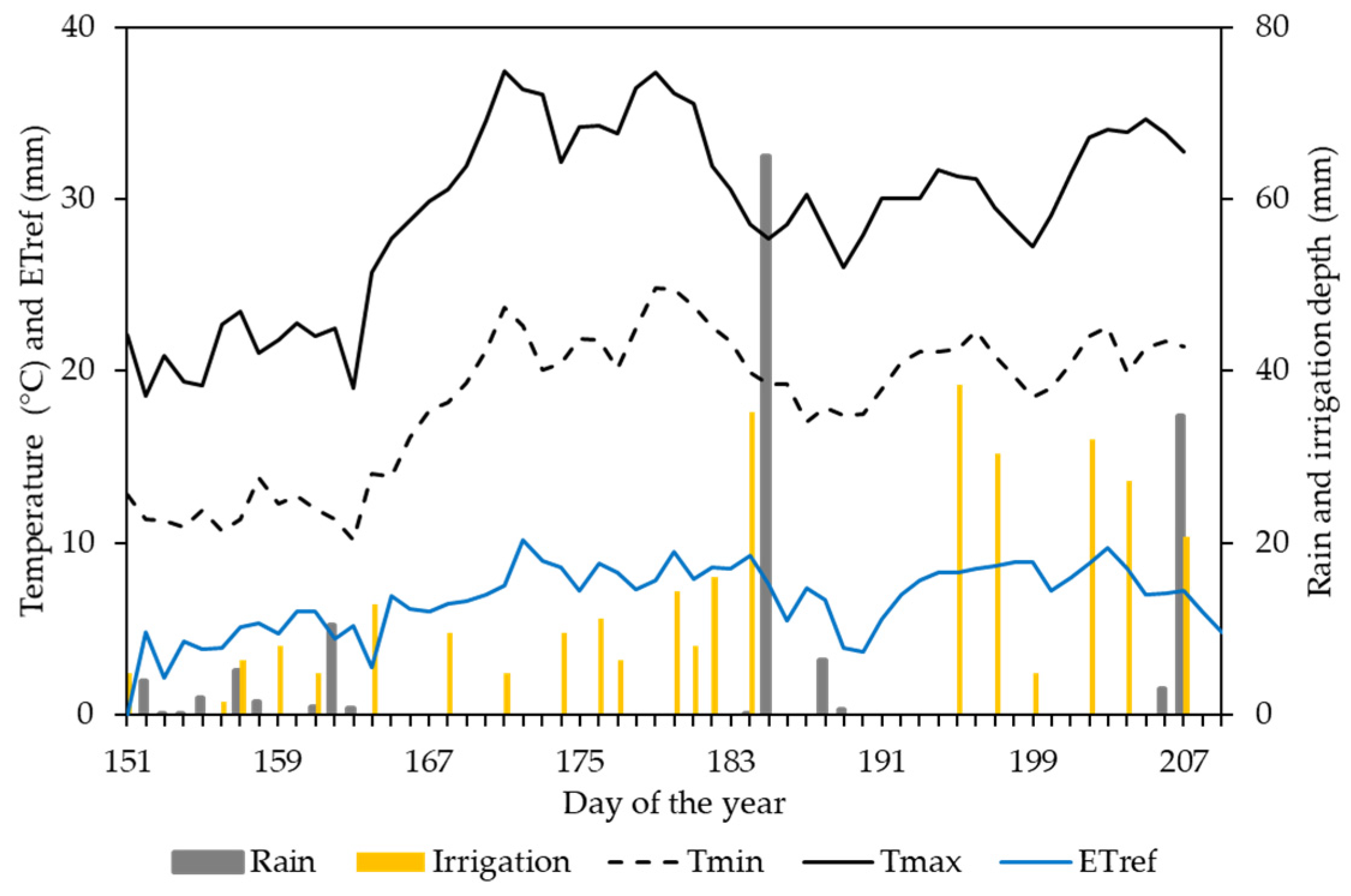
3.1. Field Meterological Characterization

The dynamics of meteorological variables (minimum and maximum temperature, reference evapotranspiration (ETref), and rainfall) recorded during the crop cycle season are shown in Figure 3. Daily temperatures reached the highest values in the last ten days of June (about 20 °C and 35 °C for minimum and maximum temperature, respectively), followed by a colder period which lasted until the end of soil monitoring. From the beginning, ETref increased from 4 to more than 10 mm in the last ten days of June, remaining higher than 7.5 mm for the remaining period except for the first ten days of July when it dropped to 4 mm. In the first 12 days the rainfall was 23 mm, followed by a dry period followed interrupted by a 65-mm event recorded on 4 July. After that, significant rainfall for soil water balance did not follow up to the end of the monitoring period, except for one episode of rainfall of about 35 mm on 26 July. Throughout the study period, against an atmospheric evaporative demand of almost 400 mm, 135 mm of rain were recorded with a corresponding water deficit of 265 mm, which made irrigation necessary to meet the transpiration demand of the watermelon.

During the monitored period, i (Equation (2)), the soil cover measured through ceptometer, increased from 0.60 to 0.85. The canopy width cw ranged from 1 to 2 m, with values of c, the correction fraction of Equation (2), between 1.2 and 2.5. The potential transpiration of Equation (2), $T_P$, calculated over the all soil surface, was 302 mm, while the adjusted potential transpiration, $T_P^{\prime }$, calculated for defining the time variable top boundary condition of monodimensional soil domain, was 631 mm.

Figure 3 shows the 21 irrigation events carried out by the farmer for a total irrigation depth of about 300 mm, with an average height of 14 mm and an irregular temporal distribution. In fact, in the first half of the observed cycle (32 days), compared with the next one, the irrigations were more frequent (one every 2.3 days) and with an average height of 8 mm. Afterward (26 days starting from 1 July), the farmer carried out less frequent irrigations (one every 3.6 days) but with a higher height (on average 27 mm).

With the TDR100 it was possible to characterize the time evolution of soil water content (Figure 4). As a result of infiltration processes, due to rain or irrigation and root uptake, under the dripper lines there were large temporal changes that, in deeper layers, were more damped and with higher values than the shallower ones. In the inter-row space, SWC remained low and almost constant until the rain event of 65 mm of 4 July; after that SWC increased and then gradually decreased. Because of this rainfall, the farmer did not irrigate for 10 days, causing the soil water reserve to be emptied for the entire monitored profile, as detected by TDR probes installed horizontally under the plant rows at 10- and 70-cm depths. These observations strongly support the hypothesis of one-dimensional fluxes along the soil profile below the plant rows. In fact, the water fluxes of the soil–plant–atmosphere’s continuum occurred mainly in a confined soil volume, well explored by the roots and placed below the plastic mulch.

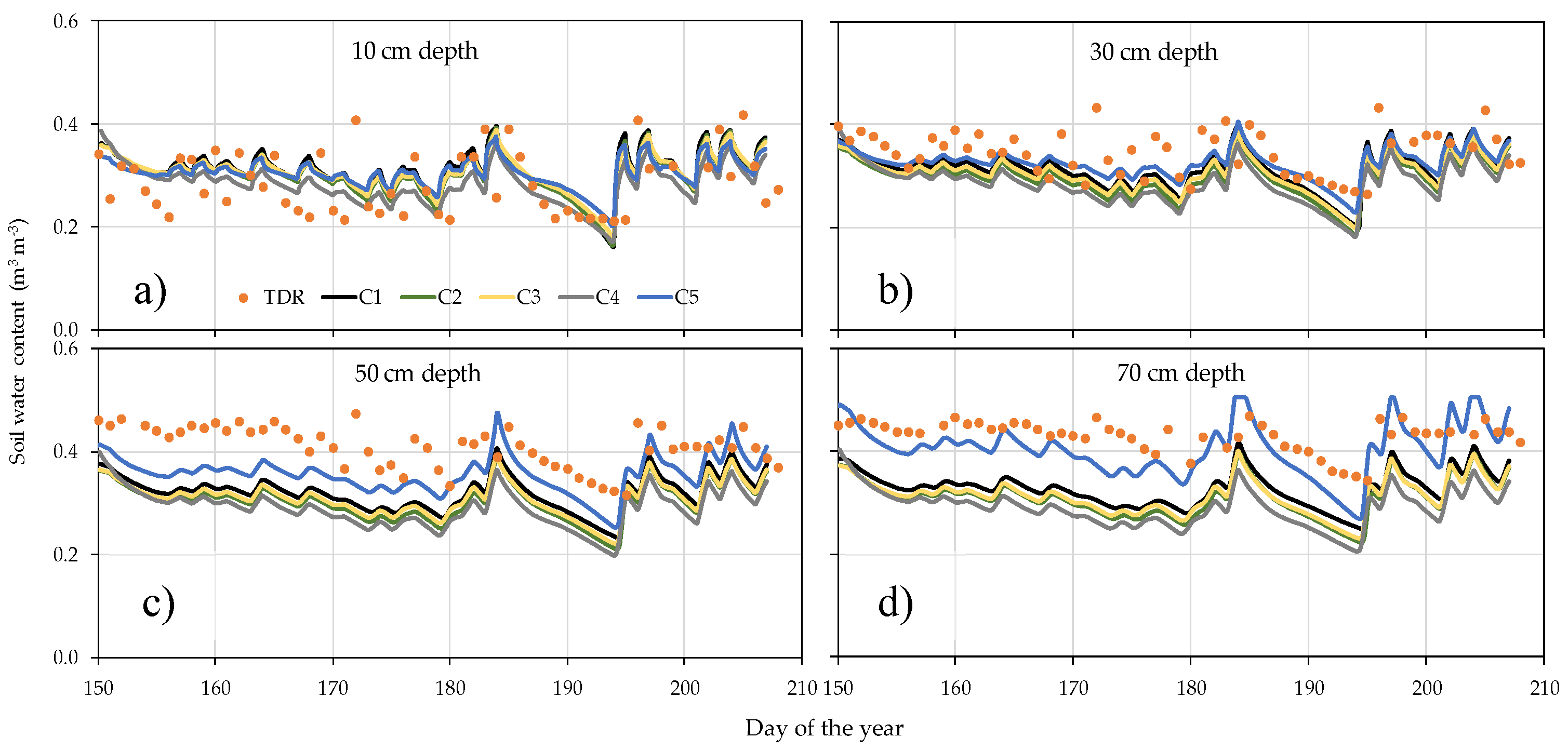
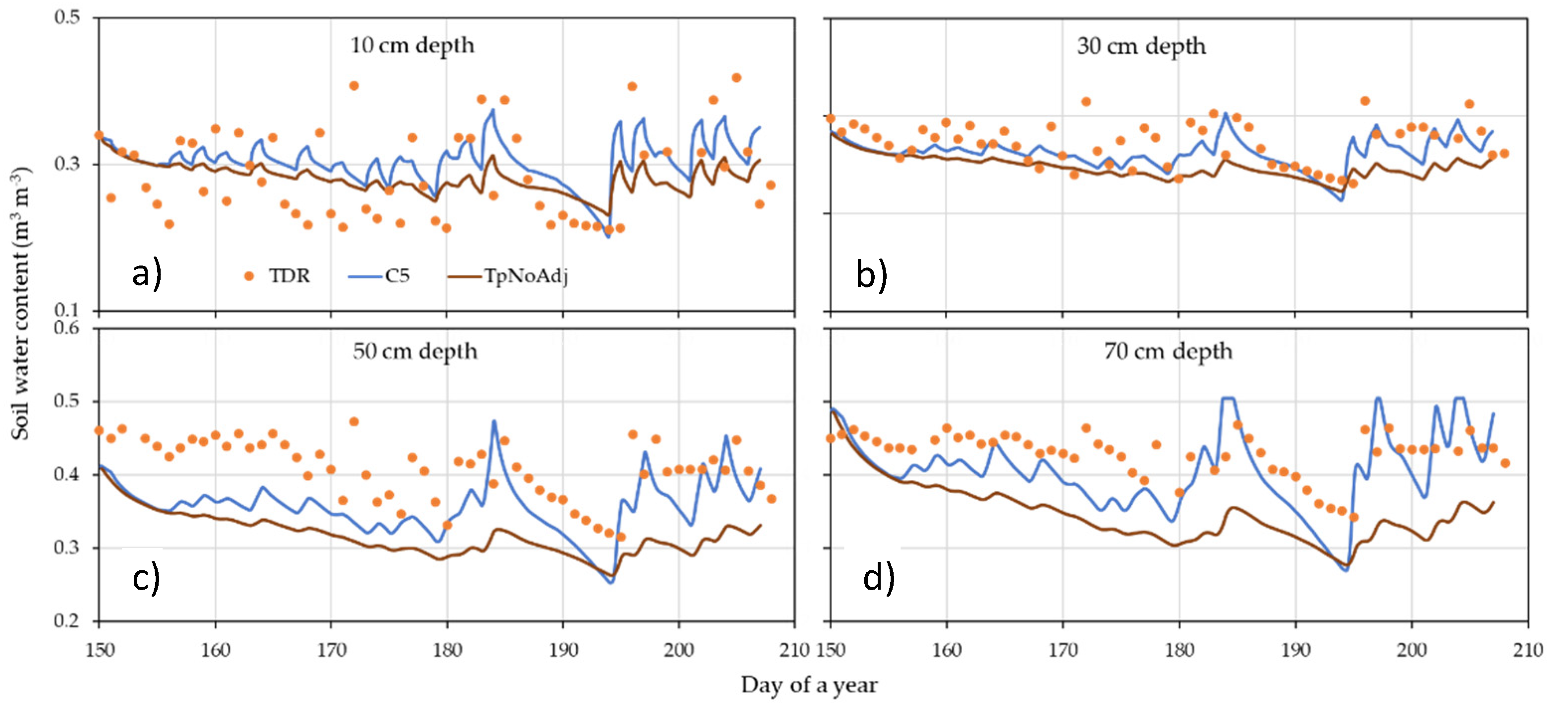
3.2. Calibration of Hydrus-1D

Comparisons between SWC measured and simulated by Hydrus-1D for the five different approaches are shown in Figure 5. Simulated data show a significant gap with those measured by TDR, affecting the entire profile and especially the deepest layers. Simulated SWC of such a layer shows an almost constant trend except for the period when the irrigation was suspended, causing a reduction of SWC due to the root water uptake. This constant SWC trend in the deepest layer led us suppose the existence of an impervious layer, characterized by a low Ks value that prevented the flux of deep percolation. Therefore, a 6-cm layer characterized by a Ks equal to 0.5 cm d⁻¹, keeping the other parameters unchanged, was inserted into the soil profile at a depth of 83 cm as shown in Figure 6.

The

Table 3. Statistical indicators comparing the performance of the five approaches in order to describe the measured soil water content.

Approach	RMSE *	rRMSE	ME	IA	CD	RM	AE	R2	a	b	SE	RI
C1	0.064	0.169	−1.74	0.622	3.28	0.157	0.060	0.81	0.105	0.858	0.022	3.95
C2	0.079	0.209	−3.19	0.548	4.76	0.199	0.075	0.81	0.128	0.825	0.023	2.18
C3	0.073	0.194	−2.60	0.569	4.11	0.184	0.070	0.82	0.102	0.895	0.022	3.41
C4	0.093	0.247	−4.85	0.493	6.44	0.237	0.090	0.78	0.156	0.770	0.024	1.00
C5	0.035	0.093	0.16	0.814	1.43	0.067	0.028	0.80	0.097	0.798	0.023	4.45
Perfect fit	0	0	1	1	1	0	0	1	0	1	0	5

*: RMSE: root mean square error; rRMSE: root mean square error; ME: modelling efficiency; IA: index of agreement; CD: coefficient of determination; RM: coefficient of residual mass; AE: mean absolute error; a: regression intercept; b: regression slope; RI: ranking index.

reports 11 out of 24 the utilized statistical indicators and the ranking index calculated to compare the performances of the five approaches to simulate the measured SWC. C5, obtained from accurate lab measurements, provided the best values for all the indicators that were closest to the optimal values shown in the last row of the Table 3.

Basically, for C5, the rRMSE value (less than 10%) was very favourable. Modelling efficiency, although significantly far from the optimal value of 1, was positive, unlike the other four approaches showing negative values (up to −4.85 of C4). The differences were high for index of agreement, coefficient of determination, residual mass, and mean absolute error, with values for C5 being 1.4, 3.2, 2.9 and 2.6 times better than the average values of the remaining approaches. However, the other approaches indicated a better regression coefficient and slope compared to C5.

The standard error was the indicator with the smallest differences between the 5 approaches, with values very close to 0.02, thus indicating a temporal variability that was independent of the set of adopted parameters. The ranking index (RI) equal to 4.45 indicated C5 as the approach that best described the SWC dynamic, followed by C1 and C3 (RI greater than 3), C2 (greater than 2) and finally C4, which had the worst performance (RI = 1). rRMSE, ME, and AE are aligned with the values obtained by Autovino et al. (2018) under olive cultivation simulated with two dimensional Hydrus-2D (in average for two years: 0.06, 0.4, and 0.02).

Figure 7 shows the time evolution of SWC as measured through TDR and simulated with the five parameter sets, at the four soil depths. The differences between simulated and measured values were quite narrowed in the shallowest layer and without relevant differences between the five approaches. Instead, such differences progressively increased with the probe installation depth. In the deepest layer, C5 was the only method to describe the SWC dynamic fairly well, unlike the other three approaches whose simulations were poor.

Figure 8 shows the comparison between the C5 approach and the TpNoAdj exercise in terms of their capacity to describe the transient soil water content of the cropping system in study. TpNoAdj does not take in account the particularity of our cropping system, which is the difference between soil surface covered by transpirating canopy, cw(t), and surface of wetted soil (0.8 m), with cw(t) >0.8 m. Therefore, the time variable conditions of the top boundary of TpNoAdj were $T_p$ (instead of $T_P^{\prime }$) and irrigation depth considering A (Equation (1)) equal to 130 × 2.5 m (instead of 130 × 0.8 m). Figure 8 shows an evident larger disagreement between soil water content measured by TDR and simulated by TpNoAdj compared to C5, above all at depths of 50 and 70 cm. Moreover, TpNoAdj tends to dampen the time variability of SWC more than C5 and erroneously compared to TDR measurements. This result is expected considering that the no-adjusted potential transpiration and irrigation depth, imposed as top boundary condition for a one-dimensional model, failed to match the large SWC changes measured by TDR in the wetted soil volume. Therefore, under the experimental conditions characterized (clay soil cultivated with melon in an intensive cropping system), the direct measurement of soil parameters was useful in order to improve the simulation capabilities of Hydrus-1D in describing the water fluxes in the “soil–plant–atmosphere” continuum. These findings have obvious implications for simulating the water fluxes in semiarid Mediterranean cropping systems, because a great debate is still current on the best choice between standard and accurate (lab) or rapid and simplified (PTFs) methods for soil hydraulic characterization. Therefore, a more in-depth discussion on this main topic of soil hydrology is reported in Section 4, “Sensitivity analysis”.

After evaluating the different capacities to simulate the soil water fluxes of the different parametrization approaches in study, we carried out a sensitivity analysis with the aim of identifying the most sensitive hydraulic parameters to describe the soil water balance. To do this, we perturbed each of the five parameters by increasing the corresponding values used in C5 by + 10% and running Hydrus-1D again. Figure 9 shows the SWC and soil pressure head (h) trends at two depths (10 and 70 cm). The perturbation of the hydraulic parameters had a significant impact in the calculation of the SWC both in the superficial and in the deep layer. θs and n were the most sensitive parameters and, for the shallowest layer, their +10% perturbation resulted in SWC variations that reached up to 45 and –30%, respectively. The impact on h occurred above all in the period with suspended irrigation (the first 10 days of July) which caused a strong reduction of SWC, especially in the 0–20 cm layer. The perturbation of θr and Ks had no effects; that of θs and n resulted in a 30% increase; and that of α in a reduction of 12%.

Figure 10 shows the sensitivity of water fluxes of infiltration, percolation, and plant uptake to hydraulic parameters. The temporal evolution of soil pressure head explored by root apparatus (hroot) is also shown. These trends confirmed what was highlighted in the previous figure, with a greater weight of two parameters of water retention function, i.e., θs and n. The variables most affected by their variations were cumulative infiltration and hroot. The perturbation of θs and n caused changes in deep percolation of +14 and −11%, respectively. Also, for the volume explored by the roots, by increasing θs and n, the greatest variations of h were found in the period of July with a damping of the fall of 12 and 35%, respectively.

As for the root water uptake, negligible variations were recorded and the most sensitive parameter was n, with a slight variation of 2.5%. Despite this small variation, the importance of two of the four parameters of the water retention function emerged, namely θs, the water content at saturation, and n, a fitting parameter that regulates the shape of the function itself. From an agronomic point of view, θs and n influence the irrigation scheduling variables, such as the irrigation height and the time interval between an irrigation and the next one.

Figure 10 also shows that, in the considered flow domain and in the two months of monitoring, against an actual infiltration of about 960 mm, there was a plant uptake of 600 mm and a percolation of 350 mm, highlighting an excess of irrigation carried out by the farmer. Finally, the 600 mm of uptake took place in a confined volume delimited by a smaller soil surface than the vegetable canopy area, as shown in Figure 1. Therefore, the uptake of 600 mm was greater than the evaporative demand of the environment of 400 mm (which refers to an entire evaporating surface) and the water absorbed by the roots was distributed over the area of vegetable canopy, corresponding to the evaporative demand and that was larger than the area of uptake.

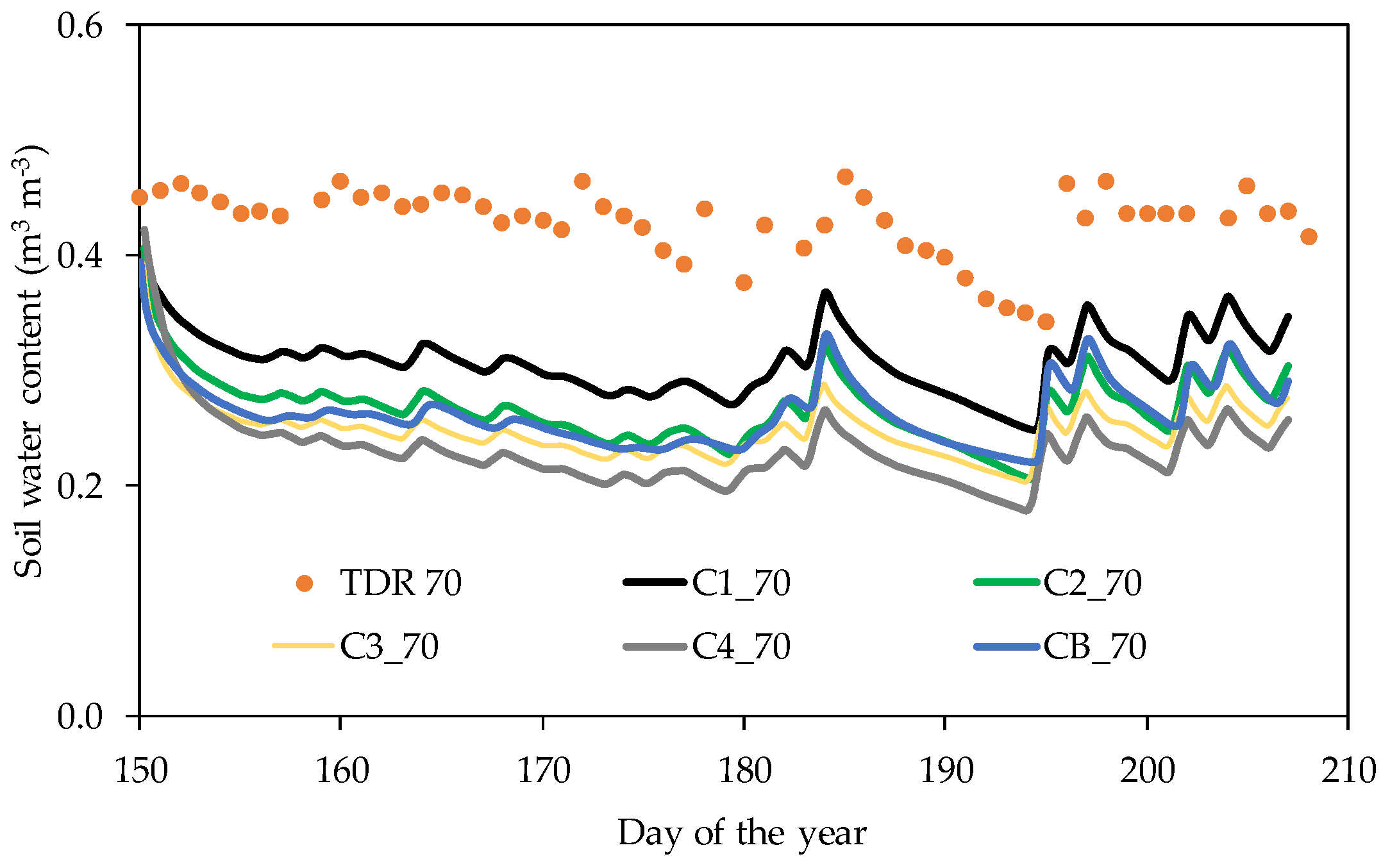
3.3. Saturated Hydraulic Conductivity Measurement Impact

Compared to the other hydraulic parameter, Ks is characterized by a very large variability [37], it changes in space and in time and, for this reason, it is a key parameter for the hydrological models based on Richards equation, as reported in the large bibliography of Šimůnek et al. [7]. However, in agricultural cropping systems, due to the soil tillage carried out for seed bed preparation, this variability can be significantly reduced compared to non-agricultural systems. Indeed, Autovino et al. [2] showed Ks values for their olive orchard system between 20 and 70 cm d⁻¹. To take in account this peculiarity, we have expanded the range of variability in the Ks sensitivity analysis, utilizing the field measurement results for a soil with similar soil textural composition. The imposed variability for Ks, from 300 to almost 4000 cm d⁻¹, had no impact on temporal evolution of SWC and h at any depths (data not shown for −30 and –50 cm), as shown in Figure 11.

With regard to the soil water fluxes, the variations were undetectable for the cumulative variables. For this reason, we considered the daily fluxes instead of the cumulative ones (Figure 12). The variations due to the Ks perturbation occurred following large rain or irrigation events and involved both infiltration and deep percolation, at the top and bottom boundary layer, respectively. In these same periods, also the plant uptake was irregularly and slightly affected. On the contrary, for hroot no impact was detected.

Therefore, with respect to the other parameters of the Mualem-van Genuchten model, Ks showed less sensitivity in influencing the state variables, h and SWC, and the main cumulative and daily fluxes, such as water infiltration, percolation, and uptake. This result should be put in relation to the fact that, in the climatic and agronomic context that we have considered, both the rains and the irrigations have not been so heavy as to create very high gradients of h along the soil profile.

4. Discussion

Horticultural crops are widespread high-income crops in Mediterranean regions but need accurate and rational management for saving water resources [38]. In this investigation, we applied an integrated experimental approach in order to optimize the water use efficiency of a typical horticultural cropping system of Southern Italy, based on drip-irrigated watermelon cultivation. For this purpose, (1) accurate and simplified methods were selected and compared to measure and estimate, respectively, the physical and hydraulic properties of the soil, (2) the model by Coelho and Or [25] was applied to estimate root length density distribution starting from TDR measurements, and (3) the Hydrus-1D software was used to model the system under study, and pros and cons of the applied methods were critically discussed below in light of the available options.

Soil hydraulic properties may be responsible for soil water content field variability, which in turn affects the spatial distribution of root density [39]. Overall, in the literature it is agreed that irrigation scheduling based on soil properties knowledge allows management of the irrigation in a more efficient way [40]. For this, a great debate is still current on the best choice between accurate-lab or simplified methods for soil hydraulic characterization, and the pros and cons have been clearly summarized in the literature [41]. In fact, experimental efforts are often linked with the financial availability and the expected accuracy. Silva Ursulino et al. [5], for example, using TDR probes and Hydrus-1D for modelling one-dimensional flow in two plots in the Gameleira Experimental River Basin, Northeast Brazil, showed that simplified estimates of soil properties by the BEST method [27] may be considered adequate to estimate the hydraulic functions, even with the final aim of modelling the water flow processes and water budget for a soil profile. However, although BEST can be considered quicker and simpler than standard methods, it can be considered more accurate if compared with common PTFs, so it could be suggested as a compromise between the two approaches. In this investigation, accurate measurements of soil hydraulic properties were obtained by the Wind’s evaporation method, coupled with infiltrations of the Uhg type. Overall, Wind’s approach is quite widespread in different experimental conditions, e.g., [42], because it provides multiple and simultaneous measurements of volumetric soil water content and soil pressure head. Moreover, it provides measurements of soil hydraulic properties from a depletion experiment involving an upward water flux that is more representative of natural hydrological processes [13]. Therefore, it is particularly suitable for agronomic applications. On the contrary, relatively worse results were obtained when PTFs of literature were used, confirming that they are useful tools, but specifically suitable for territorial-scale studies. Consequently, if the hydraulic characterization requires non-demanding soil sampling (i.e., few samples to analyze), the former approach should be suggested.

Another aspect that requires a choice a priori is linked to the approach to measure directly or to estimate quickly, and with little experimental burden, the root length density distribution. Overall, the option of digging a trench to establish the actual root development is not always feasible, especially in private farms. Application of the Coelho and Or [25] model and of the TDR probes system at multiple depths allowed us to estimate a deepening of the watermelon roots up to 70 cm of the soil profile, with about 70% of them developed in the first 50 cm. Therefore, this simplified solution seems to be applicable for estimating the watermelon root growth under drip irrigation and plastic mulch.

Finally, findings of this investigation show that the physically based Hydrus-1D model allows us to adequately simulate the water content within the framework of a typical drip-irrigated horticultural system. As a consequence, this free-software can be a viable alternative to more complex and paid license models. Moreover, since Hydrus is a very flexible type of software and allows an accurate spatial discretization of the soil, depending on the real field situations, it was possible to take into account a probable low permeability layer, which was set at an 80-cm depth according to the TDR measurements. This compact layer, which is probably linked to the pedological characteristics of the investigated soil profile, is plausible because the measured bulk density increased by about 10% from upper layers (0–20 cm) to deeper ones (21–40 cm). Consequently, considering this impervious layer was decisive for improving the model calibration performance. On the other hand, the presence of this low-permeability layer may have affected the soil pressure head distribution and, consequently, the relatively small hydraulic gradients reached. This hypothesis and the relatively low irrigation/rainfall events were addressed as the main factors for the observed low sensitivity of Ks to the main soil variables, namely soil pressure head or soil water content, and the main cumulative and daily fluxes, such as water infiltration, percolation, and water uptake. This unexpected finding deserves to be further investigated in the future with ad hoc studies.

5. Conclusions

The results of this study indicate that the physically based Hydrus-1D model allows for simulating fairly well the soil water contents measured at different distances under a typical cultivation scheme of a drip irrigated horticultural system, predicting the measured values with an average root mean square error lower than 9%. As expected: (1) the water flow domain was found to be characterized by two-dimensional pressure gradients, however (2) the fluxes of the “soil–plant–atmosphere” continuum were confined in a restricted soil volume, and (3) therefore it can be considered of one-dimensional type and can be described by a one-dimensional model such as Hydrus-1D.

Among the hydraulic parameters of the hydraulic retention and conductivity functions, it is convenient to directly determine the water content at saturation, θs, and the fitting parameters, α and n, with the laboratory or field methods reported in literature, while for the residual water content, θr, and saturated hydraulic conductivity, Ks, the pedotransfer functions can be suitable.

However, because the results obtained in this study refer to a specific cultivation system, for other physical and agronomical conditions (e.g., other textural and structural characteristics, irrigation methods with high irrigated flow rates), a direct determination of Ks with greater precision using the available measurement methods could be required for a better simulation of the soil water fluxes.

References

1. Ventrella, D.; Charfeddine, M.; Giglio, L.; Castellini, M. Application of DSSAT models for an agronomic adaptation strategy under climate change in Southern of Italy: Optimum sowing and transplanting time for winter durum wheat and tomato. Ital. J. Agron. 2012, 7, e16. [Google Scholar] [CrossRef]
2. Autovino, D.; Rallo, G.; Provenzano, G. Predicting soil and plant water status dynamic in olive orchards under different irrigation systems with Hydrus-2D: Model performance and scenario analysis. Agr. Water Manag. 2018, 203, 225–235. [Google Scholar] [CrossRef]
3. Kader, M.A.; Nakamura, K.; Senge, M.; Mojid, M.A.; Kawashima, S. Numerical simulation of water- and heat-flow regimes of mulched soil in rain-fed soybean field in central Japan. Soil Till. Res. 2019, 191, 142–155. [Google Scholar] [CrossRef]
4. Pinheiro, E.A.R.; de Jong van Lier, Q.; Inforsato, L.; Šimůnek, J. Measuring full-range soil hydraulic properties for the prediction of crop water availability using gamma-ray attenuation and inverse modeling. Agr. Water Manag. 2019, 216, 294–305. [Google Scholar] [CrossRef] [Green Version]
5. Silva Ursulino, B.; Maria Gico Lima Montenegro, S.; Paiva Coutinho, A.; Hugo Rabelo Coelho, V.; Cezar dos Santos Araújo, D.; Cláudia Villar Gusmão, A.; Martins dos Santos Neto, S.; Lassabatere, L.; Angulo-Jaramillo, R. Modelling soil water dynamics from soil hydraulic parameters estimated by an alternative method in a tropical experimental basin. Water 2019, 11, 1007. [Google Scholar] [CrossRef]
6. Di Prima, S.; Castellini, M.; Abou Najm, M.R.; Stewart, R.D.; Angulo-Jaramillo, R.; Winiarski, T.; Lassabatere, L. Experimental assessment of a new comprehensive model for single ring infiltration data. J. Hydrol. 2019, 573, 937–951. [Google Scholar] [CrossRef] [Green Version]
7. Šimůnek, J.; van Genuchten, M.T.; Šejna, M. Recent developments and applications of the HYDRUS computer software packages. Vadose Zone J. 2016, 15. [Google Scholar] [CrossRef]
8. Ventrella, D.; Moahanty, B.P.; Šimůnek, J.; Losavio, N.; van Genuchten, M.T. Use of HYDRUS-1D for simulating water and chloride transport in a bare clayey soil in presence of shallow groundwater. Soil Sci. 2000, 165, 624–631. [Google Scholar] [CrossRef]
9. Han, M.; Zhao, C.; Feng, G.; Yan, Y.; Sheng, Y. Evaluating the effects of mulch and irrigation amount on soil water distribution and root zone water balance using HYDRUS-2D. Water 2015, 7, 2622–2640. [Google Scholar] [CrossRef]
10. Yang, Q.; Zuo, H.; Xiao, X.; Wang, S.; Chen, B.; Chen, J. Modelling the effects of plastic mulch on water, heat and CO2 fluxes over cropland in an arid region. J. Hydrol. 2012, 452–453, 102–118. [Google Scholar] [CrossRef]
11. Zhang, H.; Huang, G.; Xu, X.; Xiong, Y.; Huang, Q. Estimating evapotranspiration of processing tomato under plastic mulch using the SIMDualKc model. Water 2018, 10, 1088. [Google Scholar] [CrossRef]
12. Ghazouani, H.; Autovino, D.; Rallo, G.; Rallo, G.; Provenzano, G. Using HYDRUS-2D model to assess the optimal drip lateral depth for Eggplant crop in a sandy loam soil of central Tunisia. Ital. J. Agrometeorol. 2016, 1079, 47–58. [Google Scholar]
13. Castellini, M.; Iovino, M. Pedotransfer functions for estimating soil water retention curve of Sicilian soils. Arch. Agron. Soil Sci. 2019, 65, 1401–1416. [Google Scholar] [CrossRef]
14. Schaap, M.G.; Leij, F.J.; van Genuchten, M.T. Rosetta: A computer program for estimating soil hydraulic parameters with hierarchical pedotransfer functions. J. Hydrol. 2001, 251, 163–176. [Google Scholar] [CrossRef]
15. Van Genuchten, M.T. A closed-form equation for predicting the hydraulic conductivity of unsaturated soils. Soil Sci. Soc. Am. J. 1980, 44, 892–898. [Google Scholar] [CrossRef]
16. Topp, G.C.; Davis, J.L.; Annan, A.P. Electromagnetic determination of soil water content: Measurements in coaxial transmission lines. Water Resour. Res. 1980, 16, 574–582. [Google Scholar] [CrossRef] [Green Version]
17. Allen, R.G.; Pereira, L.S.; Raes, D.; Smith, M. Crop evapotranspiration—Guidelines for computing crop water requirements. In FAO Irrigation and Drainage; Paper 56; Food and Agriculture Organization: Rome, Italy, 1998; p. 15. [Google Scholar]
18. Šimůnek, J.; Šejna, M.; Saito, H.; Sakai, M.; Van Genuchten, M.T. The HYDRUS-1D Software Package for Simulating the One-Dimensional Movement of Water, Heat, and Multiple Solutes in Variably-Saturated Media; Version 4.17; Department of Environmental Sciences University of California Riverside: Riverside, CA, USA, 2013. [Google Scholar]
19. Feddes, R.A.; Kowalik, P.J.; Zaradny, H. Simulation of field water use and crop yield. In Simulation of Field Water Use and Crop Yield. Simul. Monogr.; Pudoc: Wageningen, The Netherlands, 1978; p. 188. [Google Scholar]
20. Wind, G.P. Capillary conductivity data estimated by a simple method. In Water in the Unsaturated Zone Proc Wageningen Symp; Institute for Land and Water Management Research: Amsterdam, The Netherlands, 1969. [Google Scholar]
21. Klute, A.; Dirksen, C. Hydraulic conductivity and diffusivity: Laboratory methods. In Methods of Soil Analysis: Part 1—Physical and Mineralogical Methods; American Society of Agronomy-Soil Science Society of America: South Segoe Road, MA, USA, 1986; pp. 687–734. [Google Scholar]
22. Bagarello, V.; Castellini, M.; Iovino, M. Comparison of unconfined and confined unsaturated hydraulic conductivity. Geoderma 2007, 137, 394–400. [Google Scholar] [CrossRef]
23. Halbertsma, J.M.; Veerman, G.J. A new calculation procedure and simple set-up for the evaporation method to determine soil hydraulic functions. In Report. 88; Wageningen: Amsterdam, The Netherlands, 1994; p. 21. [Google Scholar]
24. Castellini, M.; Di Prima, S.; Iovino, M. An assessment of the BEST procedure to estimate the soil water retention curve: A comparison with the evaporation method. Geoderma 2018, 320, 82–94. [Google Scholar] [CrossRef]
25. Coelho, E.F.; Or, D. Root distribution and water uptake patterns of corn under surface and subsurface drip irrigation. Plant Soil 1999, 206, 123–136. [Google Scholar] [CrossRef]
26. Braud, I.; De Condappa, D.; Soria, J.M.; Haverkamp, R.; Angulo-Jaramillo, R.; Galle, S.; Vauclin, M. Use of scaled forms of the infiltration equation for the estimation of unsaturated soil hydraulic properties (the Beerkan method). Eur. J. Soil Sci. 2005, 56, 361–374. [Google Scholar] [CrossRef]
27. Lassabatere, L.; Angulo-Jaramillo, R.; Soria Ugalde, J.M.; Cuenca, R.; Braud, I.; Haverkamp, R. Beerkan estimation of soil transfer parameters through infiltration experiments—BEST. Soil Sci. Soc. Am. J. 2006, 70, 521. [Google Scholar] [CrossRef]
28. Stewart, R.D.; Abou Najm, M.R. A Comprehensive Model for Single Ring Infiltration I: Initial Water Content and Soil Hydraulic Properties. Soil Sci. Soc. Am. J. 2018, 82, 548–557. [Google Scholar] [CrossRef]
29. Bagarello, V.; Di Prima, S.; Iovino, M. Estimating saturated soil hydraulic conductivity by the near steady-state phase of a Beerkan infiltration test. Geoderma 2017, 303, 70–77. [Google Scholar] [CrossRef]
30. Fila, G.; Bellocchi, G.; Acutis, M.; Donatelli, M. Irene: A software to evaluate model performance. Eur. J. Agron. 2003, 18, 369–372. [Google Scholar] [CrossRef]
31. Kobayashi, K.; Salam, M.U. Comparing simulated and measured values using mean squared deviation and its components. Agron J. 2000, 92, 345–352. [Google Scholar] [CrossRef]
32. Greenwood, D.J.; Neeteson, J.J.; Draycott, A. Response of potatoes to N fertilizer: Dynamic model. Plant Soil 1985, 85, 185–203. [Google Scholar] [CrossRef]
33. Willmott, C.J.; Wicks, D.E. An Empirical method for the spatial interpolation of monthly precipitation within California. Phys. Geogr. 1980, 1, 59–73. [Google Scholar] [CrossRef]
34. Loague, K.; Green, R.E. Statistical and graphical methods for evaluating solute transport models: Overview and application. J. Contam. Hydrol. 1991, 7, 51–73. [Google Scholar] [CrossRef]
35. Shaeffer, D.L. A model evaluation methodology applicable to environmental assessment models. Ecol. Model. 1980, 8, 275–295. [Google Scholar] [CrossRef] [Green Version]
36. Ventrella, D.; Castellini, M.; Di Giacomo, E.; Giglio, L. Valutazione di diversi metodi di misura per il monitoraggio del contenuto idrico del suolo. In Proceedings of the XXXVII Conference of Italian Society of Agronomy, Il Contributo della Ricerca Agronomica all’Innovazione dei Sistemi Colturali Mediterranei, Catania, Italy, 13–14 September 2007; Cosentino, S.D., Tuttobene, R., Eds.; pp. 249–250. [Google Scholar]
37. Bagarello, V.; Baiamonte, G.; Castellini, M.; Di Prima, S.; Iovino, M. A comparison between the single ring pressure infiltrometer and simplified falling head techniques. Hydrol. Process. 2014, 28, 4843–4853. [Google Scholar] [CrossRef]
38. Fiorentino, C.; Ventrella, D.; Giglio, L.; Giacomo, E.D.; Lopez, R. Land use cover mapping of water melon and cereals in southern Italy. Ital. J. Agron. 2010, 5, 185–192. [Google Scholar] [CrossRef]
39. Rallo, G.; Provenzano, G.; Castellini, M.; Sirera, À.P. Application of EMI and FDR Sensors to assess the fraction of transpirable soil water over an olive grove. Water 2018, 10, 168. [Google Scholar] [CrossRef]
40. Liang, X.; Liakos, V.; Wendroth, O.; Vellidis, G. Scheduling irrigation using an approach based on the van Genuchten model. Agr. Water Manag. 2016, 176, 170–179. [Google Scholar] [CrossRef] [Green Version]
41. Vereecken, H.; Huisman, J.A.; Bogena, H.; Vanderborght, J.; Vrugt, J.A.; Hopmans, J.W. On the value of soil moisture measurements in vadose zone hydrology: A review. Water Resour. Res. 2008, 44, W00D06. [Google Scholar] [CrossRef]
42. Pirastru, M.; Niedda, M.; Castellini, M. Effects of maquis clearing on the properties of the soil and on the near-surface hydrological processes in a semi-arid Mediterranean environment. J. Agric. Eng. 2014, 45, 176. [Google Scholar] [CrossRef]
Figure 1. Photo of a watermelon field at Castellaneta (TA, Italy) and a schematic layout of the water/soil/plant domain. The isosceles triangle indicates the maximum root growth, the brown rectangle the soil domain in which the one-dimensional soil water fluxes take place, and the vertical grey arrows the transpirative fluxes of watermelon. cw is the canopy width measured during the monitored cropping cycle.
Water 11 01657 g001
Figure 2. Measured soil water content profiles from 5 to 13 July (a) and root density profile (b) in a watermelon field.
Water 11 01657 g002
Figure 3. Daily values of minimum and maximum temperature (Tmin and Tmax), reference evapotranspiration (ETref), rain, and irrigation.
Water 11 01657 g003
Figure 4. Hourly values of soil water content (SWC) by time domain reflectometry (TDR) probes horizontally and vertically installed at depths of 10 and 70 cm and in the middle of inter-row space. Daily rain and irrigation are also reported (from [36]).
Water 11 01657 g004
Figure 5. Comparison between measured and simulated soil water content at a 70-cm depth resulting from the five approaches.
Water 11 01657 g005
Figure 6. Soil profile discretization adopted in HYDRUS-1D. The blue, green, and brown colors indicate the first, impervious, and second layers, respectively.
Water 11 01657 g006
Figure 7. Comparison between measured (TDR) and simulated soil water content with the five approaches at five depths (from a to d) after inserting the impervious layer as specified in the text.
Water 11 01657 g007
Figure 8. Comparison between measured (TDR) and simulated soil water content at five depths (from a to d) under the C5 approach and with the “TpNoAdj” exercise described in the text.
Water 11 01657 g008
Figure 9. Temporal trend of soil pressure head (a,c) and soil water content (b,d) obtained by perturbating the van Genuchten parameters under the C5 approach.
Water 11 01657 g009
Figure 10. Temporal trend of soil infiltration (a), water uptake (b), percolation (c), and pressure head of soil root volume (d), obtained perturbating the van Genuchten parameters under the C5 approach.
Water 11 01657 g010
Figure 11. Temporal trend of pressure head (a,c) and soil water content (b,d) under the nine Ks scenarios.
Water 11 01657 g011
Figure 12. Dynamic of daily rates of soil infiltration (a), percolation (c), water uptake (d), and pressure head of soil root volume (b) under the nine Ks scenarios.
Water 11 01657 g012