Optimized Artificial Neural Networks-Based Methods for Statistical Downscaling of Gridded Precipitation Data

 ,
, 

Abstract
:1. Introduction
2. Data and Methods
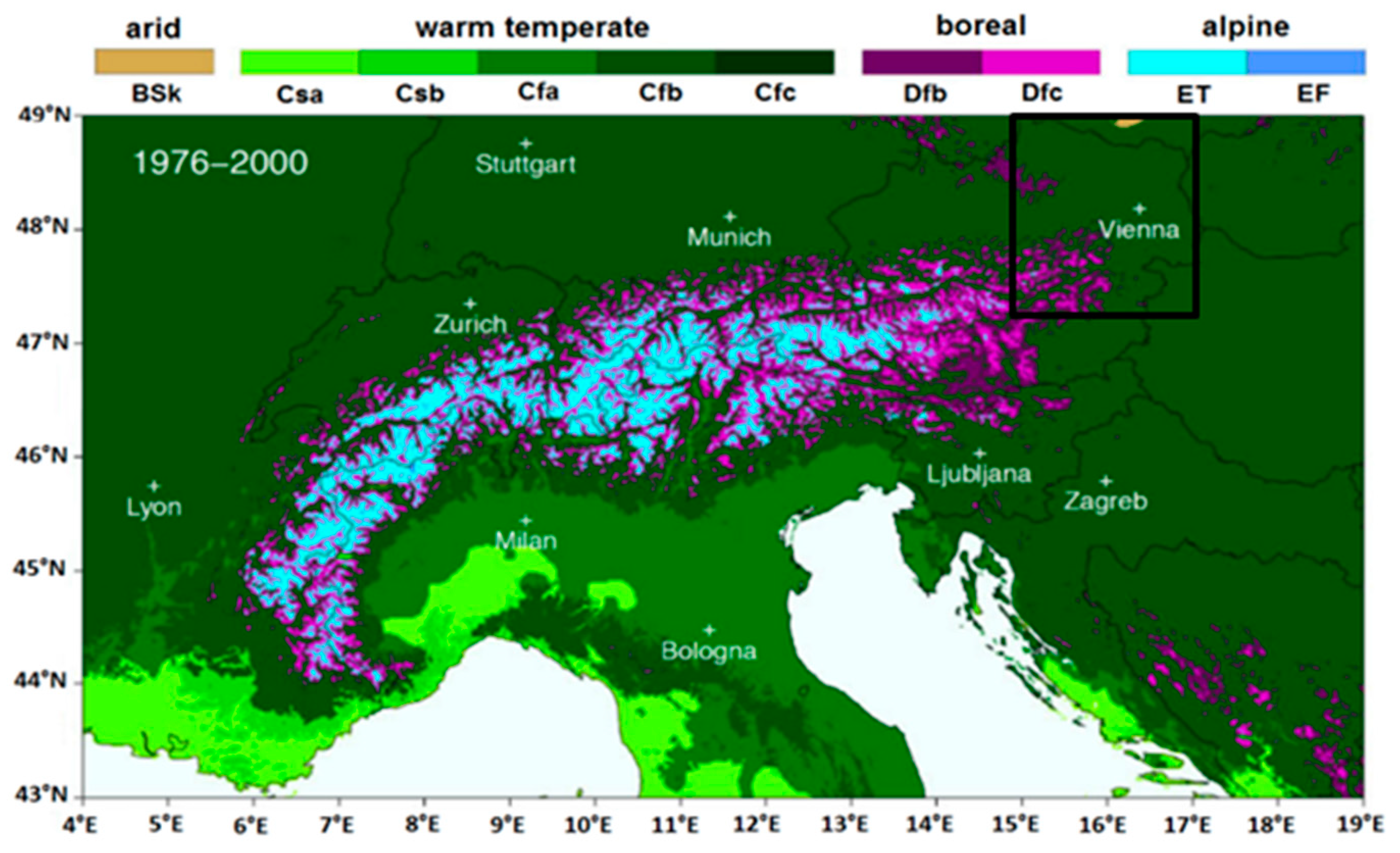
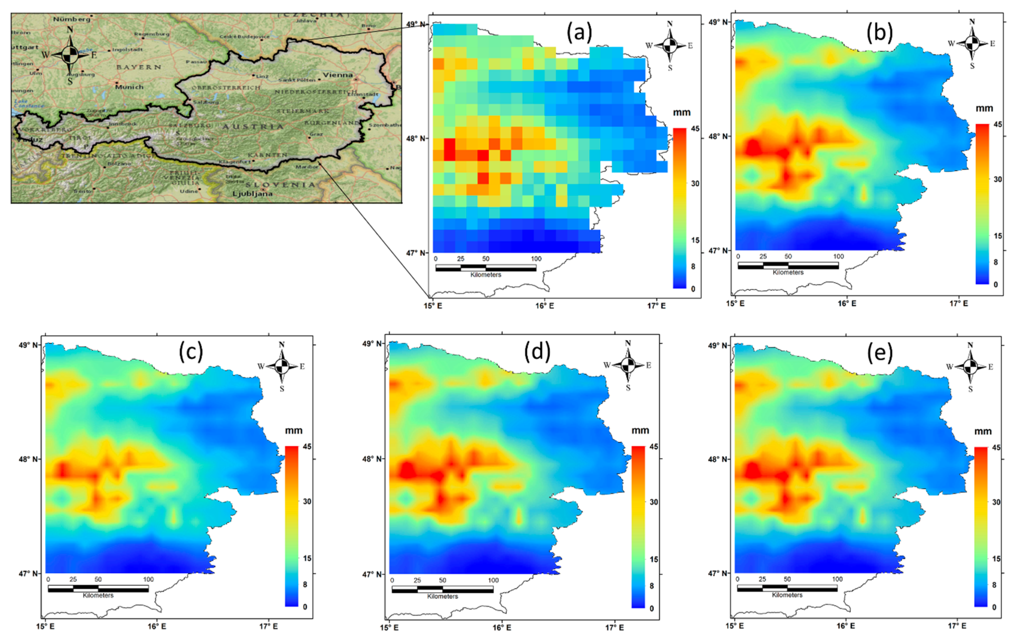
2.1. Data
2.2. Methodology
2.2.1. Artificial Neural Network (ANN)
- (a)
- 70%, 15%, and 15% of the data used for training, verification, and test of the data, respectively.
- (b)
- One hidden layer.
- (c)
- Type of the network: Feed-Forward ANN.
- (d)
- Training function: TRAINLM (Levenberg-Marquardt training algorithm).
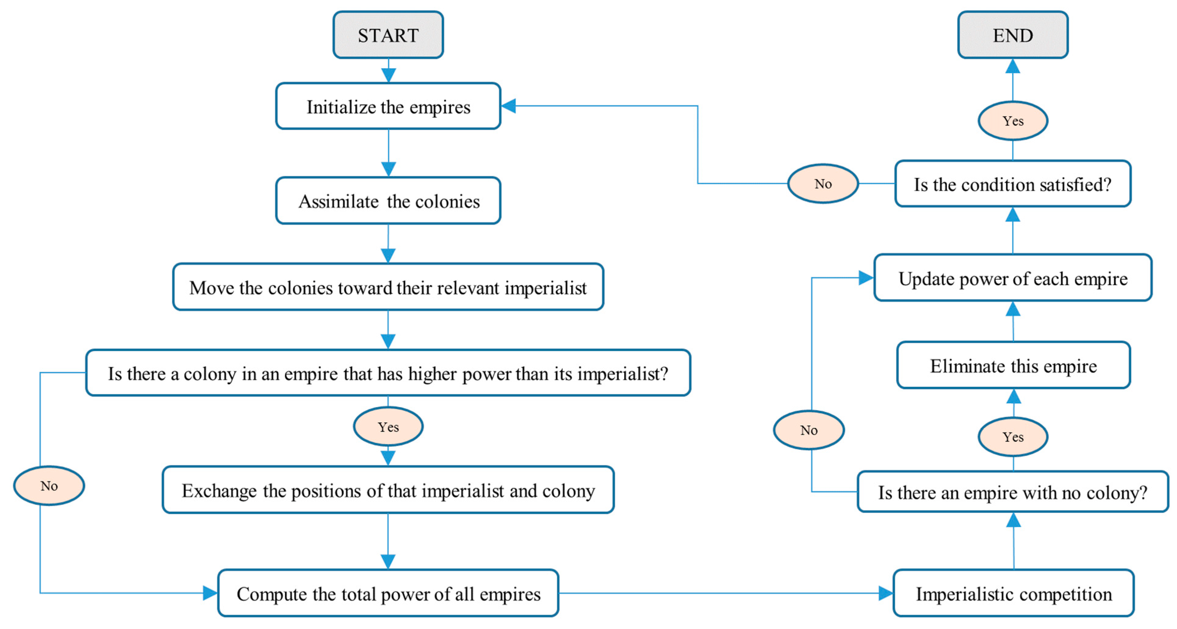
2.2.2. Imperialist Competitive Algorithm (ICA)
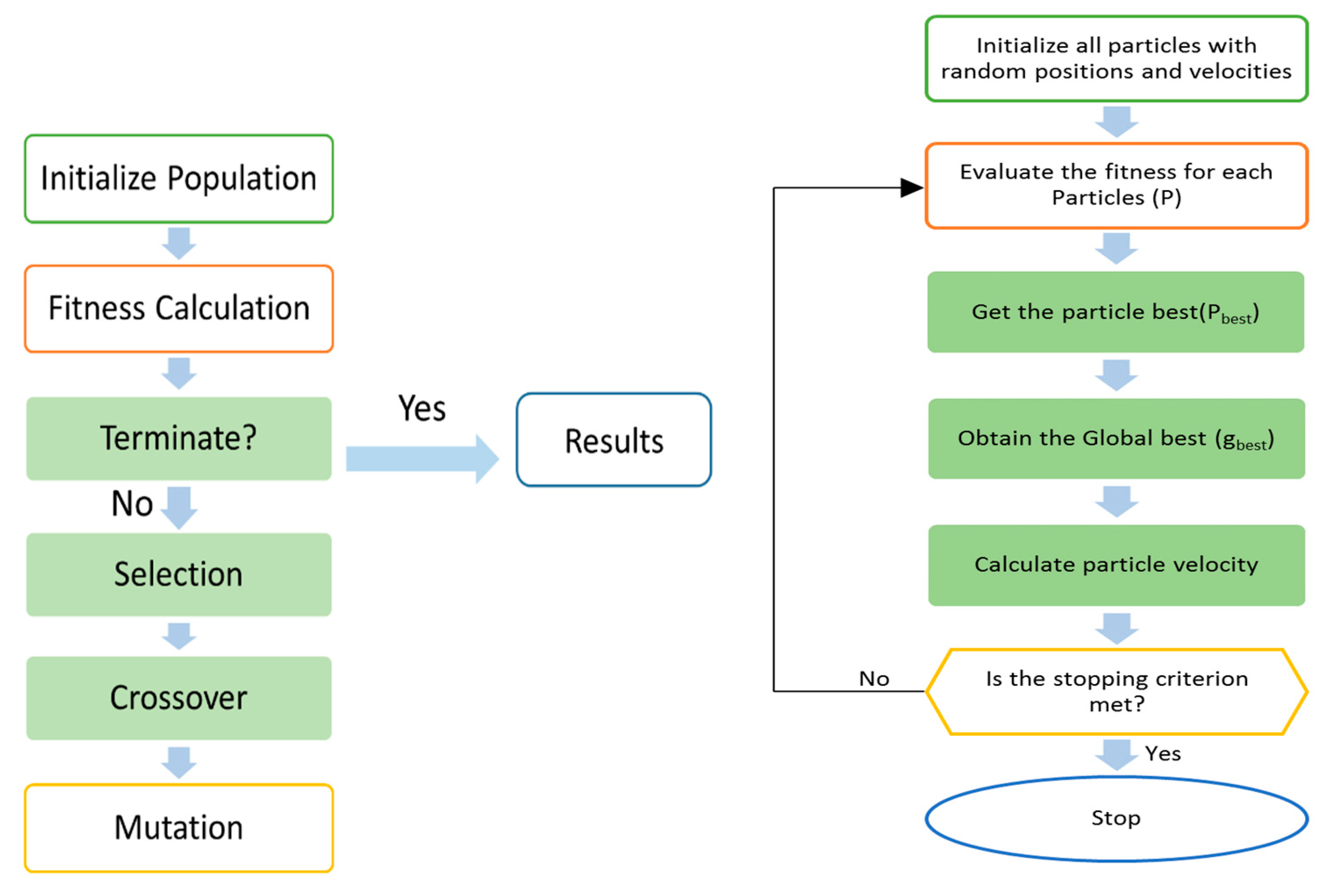
2.2.3. Genetic Algorithm (GA)
2.2.4. Particle Swarm Optimization (PSO) Algorithm
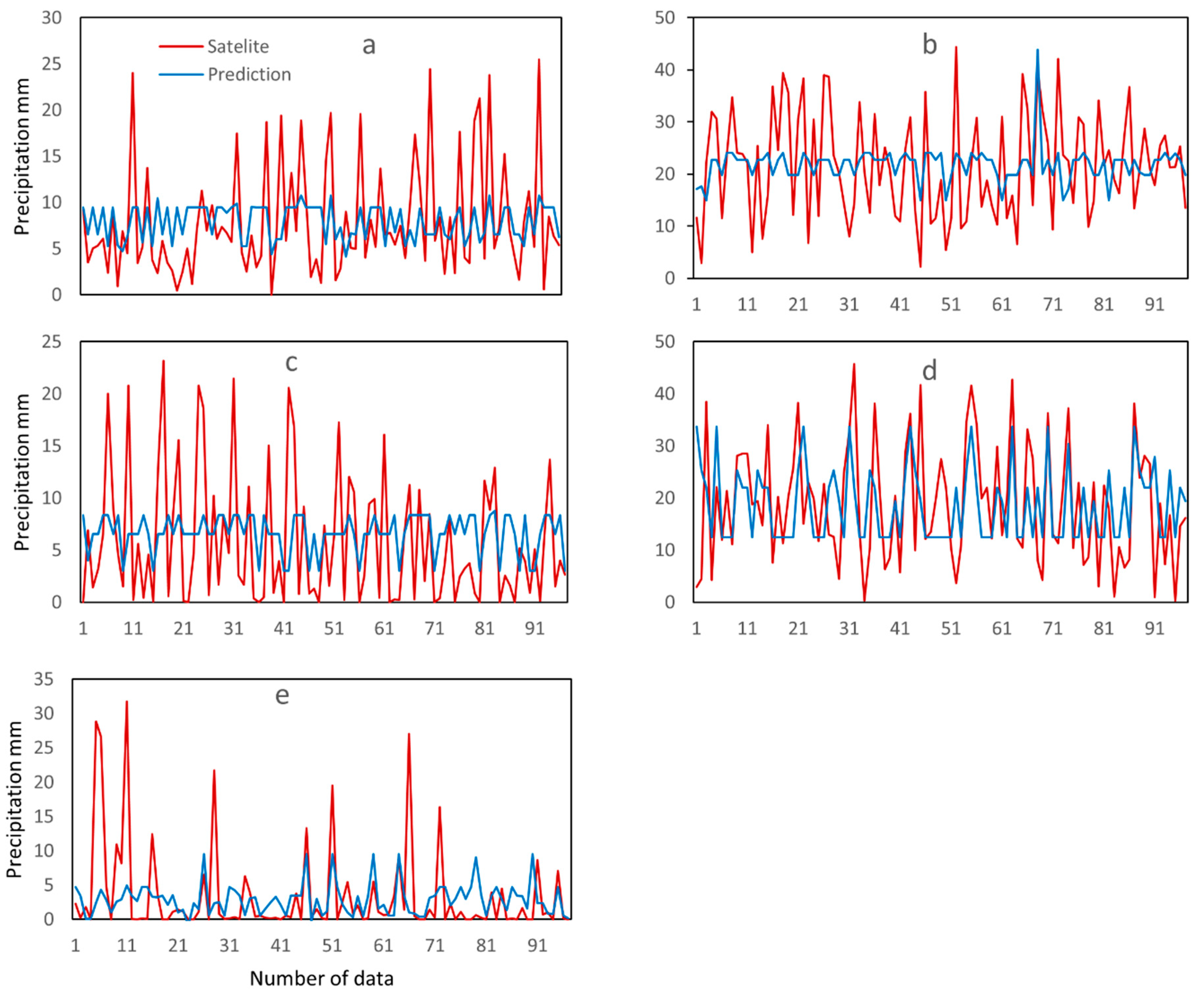
3. Results and Discussion
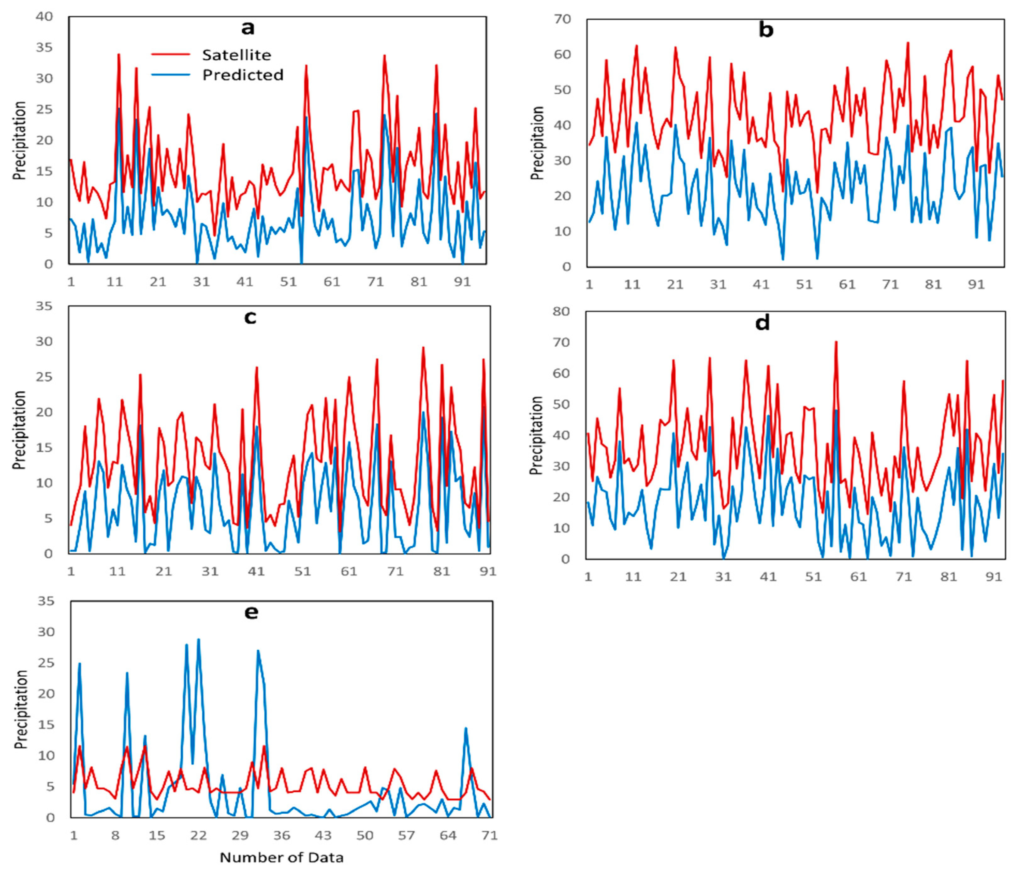
3.1. Precipitation Prediction Using ANN
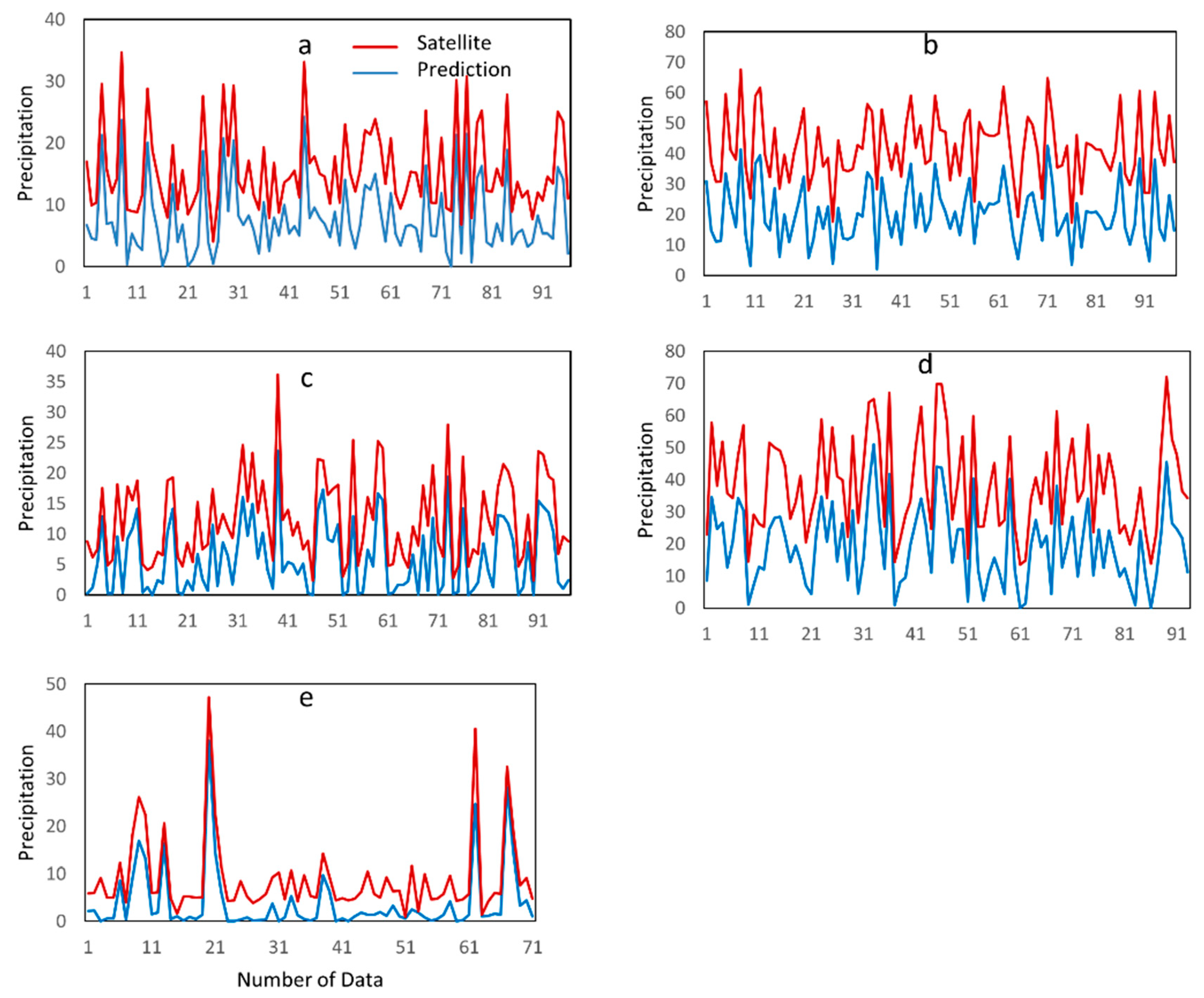
3.2. Precipitation Prediction Using Optimized ANN-based GA
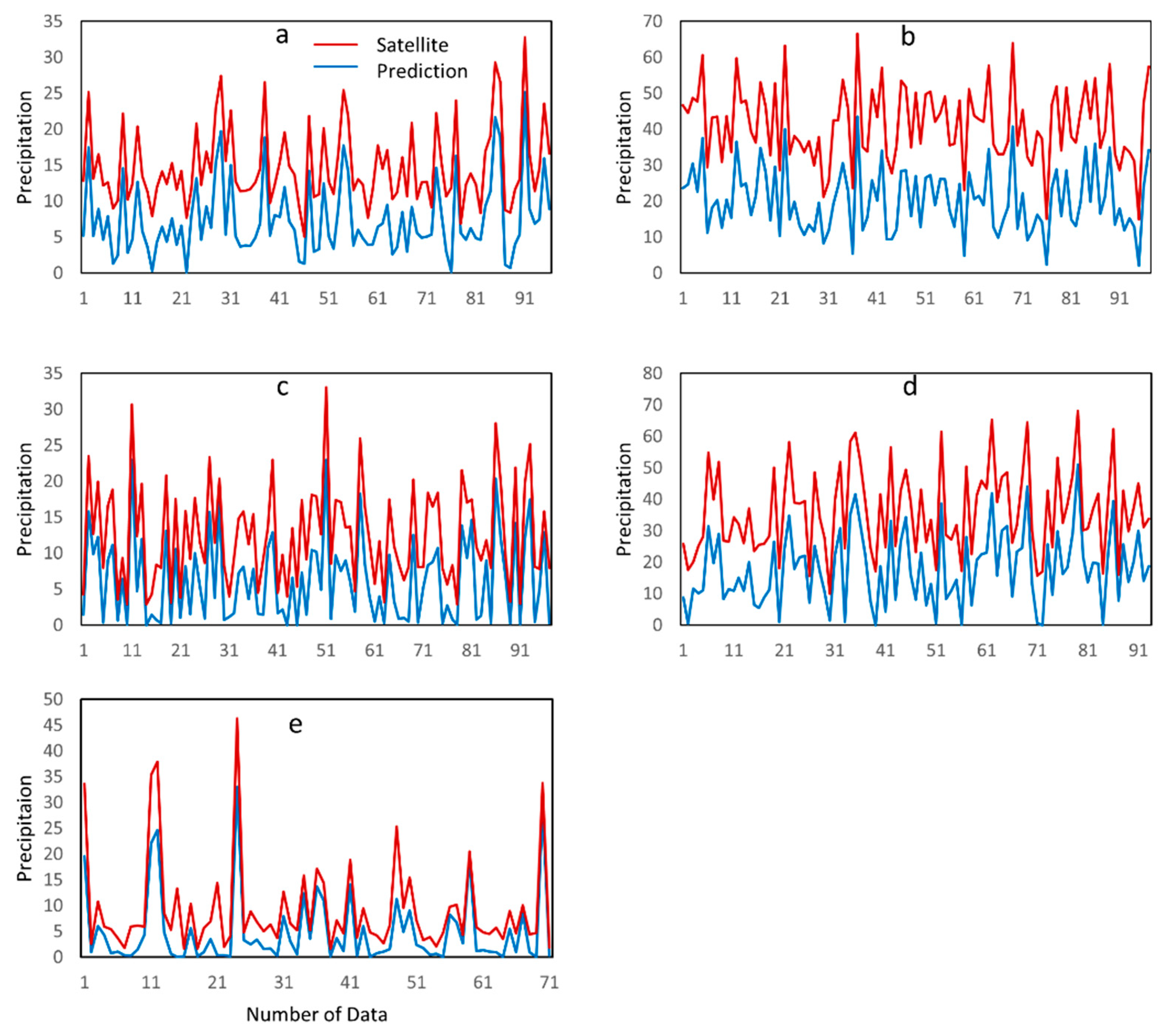
3.3. Precipitation Prediction Using Optimized ANN-based PSO
3.4. Precipitation Prediction Using Optimized ANN-based ICA
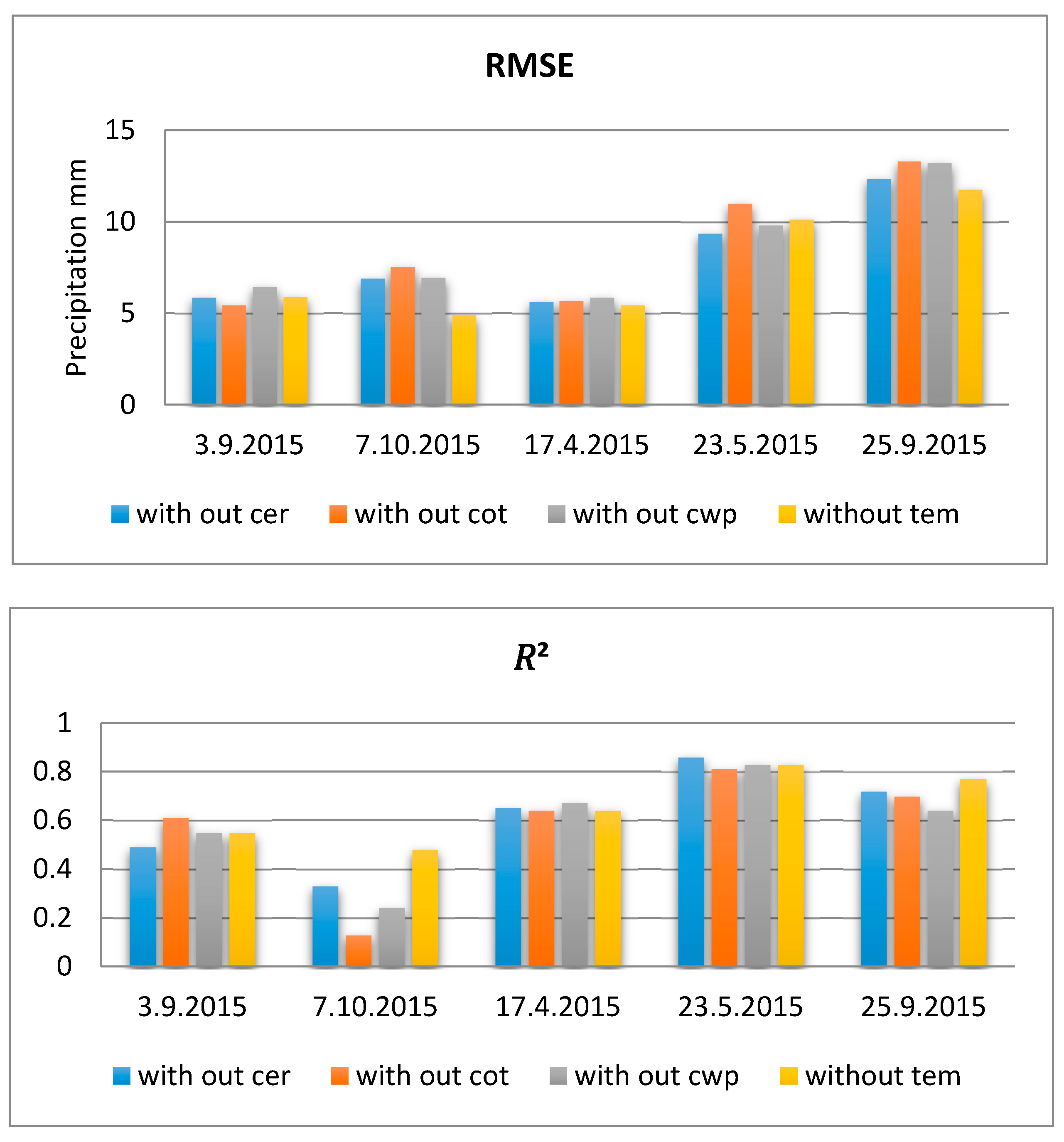
3.5. Sensitivity Analysis
4. Conclusions
Author Contributions
Funding
Acknowledgments
Conflicts of Interest
References
- Prasanna, V.; Subere, J.; Das, D.K.; Govindarajan, S.; Yasunari, T. Development of daily gridded rainfall dataset over the Ganga, Brahmaputra and Meghna river basins. Met. Apps 2014, 21, 278–293. [Google Scholar] [CrossRef]
- Gampe, D.; Ludwig, R. Evaluation of Gridded Precipitation Data Products for Hydrological Applications in Complex Topography. Hydrology 2017, 4, 53. [Google Scholar] [CrossRef]
- Tseng, K.-H.; Shum, C.K.; Lee, H.; Duan, J.; Kuo, C.; Song, S.; Zhu, W. Satellite Observed Environmental Changes over the Qinghai-Tibetan Plateau. Terr. Atmos. Ocean. Sci. 2011, 22, 229–239. [Google Scholar] [CrossRef] [Green Version]
- Chen, D.; Tian, Y.; Yao, T.; Ou, T. Satellite measurements reveal strong anisotropy in spatial coherence of climate variations over the Tibet Plateau. Sci. Rep. 2016, 6, 30304. [Google Scholar] [CrossRef] [PubMed] [Green Version]
- Beck, H.E.; Pan, M.; Roy, T.; Weedon, G.P.; Pappenberger, F.; van Dijk, A.I.J.M.; Huffman, G.J.; Adler, R.F.; Wood, E.F. Daily evaluation of 26 precipitation datasets using Stage-IV gauge-radar data for the CONUS. Hydrol. Earth Syst. Sci. 2019, 23, 207–224. [Google Scholar] [CrossRef] [Green Version]
- Karger, D.N.; Conrad, O.; Böhner, J.; Kawohl, T.; Kreft, H.; Soria-Auza, R.W.; Zimmermann, N.E.; Linder, H.P.; Kessler, M. Climatologies at high resolution for the earth’s land surface areas. Sci. Data 2017, 4, 170122. [Google Scholar] [CrossRef]
- Prakash, S. Performance assessment of CHIRPS, MSWEP, SM2RAIN-CCI, and TMPA precipitation products across India. J. Hydrol. 2019. [Google Scholar] [CrossRef]
- Zhang, A.; Xiao, L.; Min, C.; Chen, S.; Kulie, M.; Huang, C.; Liang, Z. Evaluation of latest GPM-Era high-resolution satellite precipitation products during the May 2017 Guangdong extreme rainfall event. Atmos. Res. 2019, 216, 76–85. [Google Scholar] [CrossRef]
- Sharifi, E.; Steinacker, R.; Saghafian, B. Assessment of GPM-IMERG and Other Precipitation Products against Gauge Data under Different Topographic and Climatic Conditions in Iran: Preliminary Results. Remote Sens. 2016, 8, 135. [Google Scholar] [CrossRef]
- Huffman, G.; Bolvin, D.; Nelkin, E. Integrated Multi-satellitE Retrievals for GPM (IMERG) Technical Documentation. NASA/GSFC Code 2015, 612, 2019. [Google Scholar]
- Huffman, G.J.; Bolvin, D.T.; Nelkin, E.J.; Wolff, D.B.; Adler, R.F.; Gu, G.; Hong, Y.; Bowman, K.P.; Stocker, E.F. The TRMM Multisatellite Precipitation Analysis (TMPA): Quasi-Global, Multiyear, Combined-Sensor Precipitation Estimates at Fine Scales. J. Hydrometeorol. 2007, 8, 38–55. [Google Scholar] [CrossRef]
- Dee, D.P.; Uppala, S.M.; Simmons, A.J.; Berrisford, P.; Poli, P.; Kobayashi, S.; Andrae, U.; Balmaseda, M.A.; Balsamo, G.; Bauer, P.; et al. The ERA-Interim reanalysis: Configuration and performance of the data assimilation system. Q. J. R. Meteorol. Soc. 2011, 137, 553–597. [Google Scholar] [CrossRef]
- Sharifi, E.; Steinacker, R.; Saghafian, B. Multi time-scale evaluation of high-resolution satellite-based precipitation products over northeast of Austria. Atmos. Res. 2018, 206, 46–63. [Google Scholar] [CrossRef]
- Tao, K.; Barros, A.P. Using Fractal Downscaling of Satellite Precipitation Products for Hydrometeorological Applications. J. Atmos. Ocean. Technol. 2010, 27, 409–427. [Google Scholar] [CrossRef] [Green Version]
- Sharifi, E.; Steinacker, R.; Saghafian, B. Hourly Comparison of GPM-IMERG-Final-Run and IMERG-Real-Time (V-03) over a Dense Surface Network in Northeastern Austria. In Proceedings of the European Geosciences Union General Assembly, Vienna, Austria, 23–28 April 2017. [Google Scholar]
- Sharifi, E.; Saghafian, B.; Steinacker, R. Copula-based Stochastic Uncertainty Analysis of Satellite Precipitation Products. J. Hydrol. 2019. [Google Scholar] [CrossRef]
- Coulibaly, P.; Dibike, Y.B.; Anctil, F. Downscaling Precipitation and Temperature with Temporal Neural Networks. J. Hydrometeorol. 2005, 6, 483–496. [Google Scholar] [CrossRef]
- Salimi, A.; Karami, H.; Farzin, S.; Hassanvand, M.; Azad, A.; Kisi, O. Design of water supply system from rivers using artificial intelligence to model water hammer. ISH J. Hydraul. Eng. 2019, 20, 1–10. [Google Scholar] [CrossRef]
- Hassanvand, M.R.; Karami, H.; Mousavi, S.-F. Investigation of neural network and fuzzy inference neural network and their optimization using meta-algorithms in river flood routing. Nat. Hazards 2018, 94, 1057–1080. [Google Scholar] [CrossRef]
- Khan, K.; Sahai, A. A Comparison of BA, GA, PSO, BP and LM for Training Feed forward Neural Networks in e-Learning Context. IJISA 2012, 4, 23–29. [Google Scholar] [CrossRef]
- Such, F.P.; Madhavan, V.; Conti, E.; Lehman, J.; Stanley, K.O.; Clune, J. Deep Neuroevolution: Genetic Algorithms Are a Competitive Alternative for Training Deep Neural Networks for Reinforcement Learning. arXiv 2017, arXiv:1712.06567v3. [Google Scholar]
- Sharifi, E.; Saghafian, B.; Steinacker, R. Downscaling Satellite Precipitation Estimates With Multiple Linear Regression, Artificial Neural Networks, and Spline Interpolation Techniques. J. Geophys. Res. Atmos. 2019, 75, 606. [Google Scholar] [CrossRef]
- Immerzeel, W.W.; Rutten, M.M.; Droogers, P. Spatial downscaling of TRMM precipitation using vegetative response on the Iberian Peninsula. Remote Sens. Environ. 2009, 113, 362–370. [Google Scholar] [CrossRef]
- Platnick, S.; Meyer, K.G.; King, M.D.; Wind, G.; Amarasinghe, N.; Marchant, B.; Arnold, G.T.; Zhang, Z.; Hubanks, P.A.; Holz, R.E.; et al. The MODIS cloud optical and microphysical products: Collection 6 updates and examples from Terra and Aqua. IEEE Trans. Geosci. Remote Sens. 2017, 55, 502–525. [Google Scholar] [CrossRef]
- Retalis, A.; Tymvios, F.; Katsanos, D.; Michaelides, S. Downscaling CHIRPS precipitation data: An artificial neural network modelling approach. Int. J. Remote Sens. 2017, 38, 3943–3959. [Google Scholar] [CrossRef]
- Copernicus Climate Change Service (C3S). Fifth Generation of ECMWF Atmospheric Reanalyses of the Global Climate; Copernicus Climate Change Service. 2017. Available online: https://cds.climate.copernicus.eu/cdsapp#!/home (accessed on 10 August 2019).
- Rubel, F.; Brugger, K.; Haslinger, K.; Auer, I. The climate of the European Alps: Shift of very high resolution Köppen-Geiger climate zones 1800–2100. Metz 2017, 26, 115–125. [Google Scholar] [CrossRef]
- Platnick, S.; King, M.D.; Meyer, K.G.; Wind, G.; Amarasinghe, N.; Marchant, B.; Arnold, G.T.; Zhang, Z.; Hubanks, P.; Ridgway, B.; et al. MODIS Cloud Optical Properties: User Guide for the Collection 6 Level-2 MOD06/MYD06 Product and Associated Level-3 Datasets. 2015. Available online: https://modis-images.gsfc.nasa.gov/_docs/C6MOD06OPUserGuide.pdf (accessed on 10 August 2019).
- Alexakis, D.D.; Tsanis, I.K. Comparison of multiple linear regression and artificial neural network models for downscaling TRMM precipitation products using MODIS data. Environ. Earth Sci. 2016, 75, 606. [Google Scholar] [CrossRef]
- Park, N.-W. Spatial Downscaling of TRMM Precipitation Using Geostatistics and Fine Scale Environmental Variables. Adv. Meteorol. 2013, 2013, 1–9. [Google Scholar] [CrossRef]
- Xu, G.; Xu, X.; Liu, M.; Sun, A.; Wang, K. Spatial Downscaling of TRMM Precipitation Product Using a Combined Multifractal and Regression Approach: Demonstration for South China. Water 2015, 7, 3083–3102. [Google Scholar] [CrossRef] [Green Version]
- He, X.; Chaney, N.W.; Schleiss, M.; Sheffield, J. Spatial downscaling of precipitation using adaptable random forests. Water Resour. Res. 2016, 52, 8217–8237. [Google Scholar] [CrossRef]
- Darji, M.P.; Dabhi, V.K.; Prajapati, H.B. Rainfall forecasting using neural network: A survey. In Proceedings of the 2015 International Conference on Advances in Computer Engineering and Applications (ICACEA), Ghaziabad, India, 19–20 March 2015; pp. 706–713, ISBN 978-1-4673-6911-4. [Google Scholar]
- Coulibaly, P.; Anctil, F.; Bobée, B. Daily reservoir inflow forecasting using artificial neural networks with stopped training approach. J. Hydrol. 2000, 230, 244–257. [Google Scholar] [CrossRef]
- Bishop, C.M. Neural Networks for Pattern Recognition; Clarendon Press: Oxford, UK, 1995; ISBN 0198538642. [Google Scholar]
- Atashpaz-Gargari, E.; Lucas, C. Imperialist competitive algorithm: An algorithm for optimization inspired by imperialistic competition. In Proceedings of the 2007 IEEE Congress on Evolutionary Computation, Singapore, 25–28 September 2007; pp. 4661–4667, ISBN 978-1-4244-1339-3. [Google Scholar]
- Shamshirband, S.; Gocić, M.; Petković, D.; Javidnia, H.; Ab Hamid, S.H.; Mansor, Z.; Qasem, S.N. Clustering project management for drought regions determination: A case study in Serbia. Agric. For. Meteorol. 2015, 200, 57–65. [Google Scholar] [CrossRef]
- McCall, J. Genetic algorithms for modelling and optimisation. J. Comput. Appl. Math. 2005, 184, 205–222. [Google Scholar] [CrossRef]
- Krohling, R.A.; Rey, J.P. Design of optimal disturbance rejection PID controllers using genetic algorithms. IEEE Trans. Evol. Comput. 2001, 5, 78–82. [Google Scholar] [CrossRef]
- Wan, W.; Birch, J.B. An Improved Hybrid Genetic Algorithm with a New Local Search Procedure. J. Appl. Math. 2013, 2013, 1–10. [Google Scholar] [CrossRef] [Green Version]
- Sette, S.; Boullart, L. Genetic programming: Principles and applications. Eng. Appl. Artif. Intell. 2001, 14, 727–736. [Google Scholar] [CrossRef]
- Kennedy, J.; Eberhart, R. Particle swarm optimization. In Proceedings of the ICNN’95-International Conference on Neural Networks, Perth, WA, Australia, 27 November–1 December 1995; pp. 1942–1948, ISBN 0-7803-2768-3. [Google Scholar]
- Hassanvand, M.R.; Karami, H.; Mousavi, S.-F. Use of multi-criteria decision-making for selecting spillway type and optimizing dimensions by applying the harmony search algorithm: Qeshlagh Dam Case Study. Lakes Reserve 2018, 27, 111. [Google Scholar] [CrossRef]


| Temporal Resolution | Spatial Resolution | Spatial Coverage | Parameter | |
|---|---|---|---|---|
| IMERG | 30 min | 0.1° | 60° N-S | Precipitation |
| MODIS | 1–2 images daily | 1 km | 90° N-S | CER, CWP, and COT |
| ERA5 | Hourly | 0.1° | 90° N-S | Temperature |
| Structure | Train Function | Functions | |
|---|---|---|---|
| Parameter | 25 20 output | LM | Tansig purelin |
| Population | Crossover Rate | Mutation Rate | Number of Irritation | Structure | |
|---|---|---|---|---|---|
| Parameter | 50 | 0.7 | 0.1 | 1000 | 25–20 output |
| Swarm Size | Max Iteration | Structure | |
|---|---|---|---|
| Parameter | 300 | 60 | 25–20 output |
| Number of Country | Number of Imperialism | Number of Decades | Revolution | |
|---|---|---|---|---|
| Parameter | 150 | 10 | 50 | 0.1 |
| Method | Index | Days | |||||
|---|---|---|---|---|---|---|---|
| 17 April 2015 | 23 May 2015 | 03 September 2015 | 25 September 2015 | 07 October 2015 | Average | ||
| ANN | RMSE | 5.84 | 9.69 | 6.13 | 11.81 | 6.52 | 8 |
| ANN-GA | 4.96 | 8.75 | 5.4 | 11.32 | 6.82 | 7.45 | |
| ANN-PSO | 5.62 | 8.85 | 5.3 | 11.41 | 6.44 | 7.52 | |
| ANN-ICA | 5.26 | 8.4 | 5.69 | 10.74 | 6.19 | 7.3 | |
| ANN | MAE | 6.21 | 6.22 | 8.01 | 6.98 | 6.21 | 6.726 |
| ANN-GA | 8.61 | 8.81 | 7.73 | 8.06 | 6.48 | 7.9 | |
| ANN-PSO | 6.06 | 6.09 | 6.09 | 6.08 | 4.95 | 5.8 | |
| ANN-ICA | 6.06 | 6.21 | 6.21 | 5.8 | 4.95 | 5.8 | |
| ANN | R2 | 0.65 | 0.69 | 0.49 | 0.7 | 0.25 | 0.56 |
| ANN-GA | 0.67 | 0.86 | 0.62 | 0.71 | 0.35 | 0.64 | |
| ANN-PSO | 0.67 | 0.67 | 0.6 | 0.75 | 0.36 | 0.61 | |
| ANN-ICA | 0.67 | 0.86 | 0.56 | 0.75 | 0.48 | 0.67 | |
| ANN | Bias | −0.01 | 0.03 | 0.52 | −0.1 | −0.27 | 0.17 |
| ANN-GA | −1.27 | 0.91 | 0.21 | 0.88 | −1.06 | −0.07 | |
| ANN-PSO | −0.08 | 1.4 | 0.58 | −0.32 | 1.18 | 0.55 | |
| ANN-ICA | 0.07 | −0.75 | −0.1 | −0.06 | 0.46 | −0.07 | |
| Methods | Index | Days | |||||
|---|---|---|---|---|---|---|---|
| 17 April 2015 | 23 May 2015 | 03 September 2015 | 25 September 2015 | 07 October 2015 | Average | ||
| 2.27 | −10.84 | −8.98 | 9.85 | −1.29 | −1.80 | ||
| 1.77 | −7.92 | −4.45 | −0.27 | −7.86 | −3.75 | ||
| 1.74 | –7.66 | −4.44 | −0.26 | −7.84 | −3.69 | ||
| 1.70 | −7.78 | 0.92 | −0.28 | −7.60 | −2.61 | ||
| Bias (mm) | 1.74 | −7.66 | −4.44 | −0.26 | −7.84 | −3.69 | |
| 0.59 | −12.20 | −2.39 | 0.82 | 1.60 | −2.32 | ||
| –0.43 | −10.42 | −5.54 | 4.68 | −5.22 | −3.39 | ||
| –0.29 | −10.85 | −5.23 | 4.74 | −3.51 | −3.03 | ||
| –1.59 | −10.58 | −5.70 | 4.87 | −5.54 | −3.71 | ||
| 0.65 | 0.51 | 0.25 | 0.16 | -0.07 | 0.30 | ||
| 0.66 | 0.43 | 0.73 | 0.75 | 0.22 | 0.56 | ||
| 0.69 | 0.42 | 0.74 | 0.76 | 0.23 | 0.57 | ||
| 0.69 | 0.44 | −0.69 | 0.76 | 0.39 | 0.32 | ||
| CC | 0.69 | 0.44 | 0.74 | 0.76 | 0.23 | 0.57 | |
| 0.14 | 0.19 | 0.30 | 0.15 | −0.04 | 0.15 | ||
| 0.08 | −0.04 | −0.32 | −0.40 | 0.15 | −0.11 | ||
| 0.42 | 0.10 | 0.14 | −0.07 | −0.12 | 0.09 | ||
| 0.29 | 0.06 | −0.41 | −0.33 | 0.17 | −0.04 | ||
| 4.26 | 12.58 | 9.86 | 13.07 | 10.96 | 10.14 | ||
| 3.93 | 11.06 | 5.45 | 4.78 | 7.87 | 6.62 | ||
| 3.75 | 10.56 | 5.35 | 4.79 | 7.86 | 6.46 | ||
| 3.75 | 10.56 | 13.81 | 4.79 | 7.69 | 8.12 | ||
| MAE (mm) | 3.75 | 10.56 | 5.35 | 4.79 | 7.86 | 6.46 | |
| 5.28 | 13.07 | 7.26 | 14.41 | 10.29 | 10.06 | ||
| 3.84 | 11.32 | 8.99 | 12.01 | 6.01 | 8.43 | ||
| 3.45 | 11.86 | 8.44 | 10.28 | 7.03 | 8.21 | ||
| 3.70 | 11.31 | 9.02 | 10.47 | 6.27 | 8.15 | ||
| 6.28 | 15.15 | 12.97 | 17.37 | 15.76 | 13.50 | ||
| 5.39 | 13.53 | 7.84 | 7.10 | 10.31 | 8.84 | ||
| 5.33 | 12.64 | 7.77 | 7.10 | 10.31 | 8.63 | ||
| 5.33 | 12.64 | 15.67 | 7.10 | 9.88 | 10.12 | ||
| RMSE (mm) | 5.33 | 12.64 | 7.77 | 7.10 | 10.31 | 8.63 | |
| 7.12 | 15.91 | 9.45 | 20.37 | 12.45 | 13.06 | ||
| 5.32 | 14.57 | 11.63 | 14.53 | 8.59 | 10.93 | ||
| 4.81 | 14.82 | 10.85 | 12.79 | 10.61 | 10.77 | ||
| 5.30 | 14.57 | 11.77 | 12.85 | 8.76 | 10.65 |
| DAYS | ERROR | Without CER | Without COT | Without CWP | Without TEM |
|---|---|---|---|---|---|
| 03 September 2015 | RMSE | 5.86 | 5.45 | 6.46 | 5.92 |
| MAE | 6.21 | 6.21 | 6.21 | 6.21 | |
| R2 | 0.49 | 0.61 | 0.55 | 0.55 | |
| 07 October 2015 | RMSE | 6.9 | 7.54 | 6.95 | 4.89 |
| MAE | 8.36 | 8.36 | 8.36 | 8.36 | |
| R2 | 0.33 | 0.13 | 0.24 | 0.48 | |
| 17 April 2015 | RMSE | 5.64 | 5.7 | 5.86 | 5.45 |
| MAE | 6.06 | 6.06 | 6.06 | 6.06 | |
| R2 | 0.65 | 0.64 | 0.67 | 0.64 | |
| 23 May 2015 | RMSE | 9.39 | 11.01 | 9.82 | 10.14 |
| MAE | 6.04 | 6.04 | 6.04 | 6.04 | |
| R2 | 0.86 | 0.81 | 0.83 | 0.83 | |
| 25 September 2015 | RMSE | 12.39 | 13.32 | 13.25 | 11.79 |
| MAE | 6.08 | 6.08 | 6.08 | 6.08 | |
| R2 | 0.72 | 0.7 | 0.64 | 0.77 |
© 2019 by the authors. Licensee MDPI, Basel, Switzerland. This article is an open access article distributed under the terms and conditions of the Creative Commons Attribution (CC BY) license (http://creativecommons.org/licenses/by/4.0/).
Share and Cite
Salimi, A.H.; Masoompour Samakosh, J.; Sharifi, E.; Hassanvand, M.R.; Noori, A.; von Rautenkranz, H. Optimized Artificial Neural Networks-Based Methods for Statistical Downscaling of Gridded Precipitation Data. Water 2019, 11, 1653. https://doi.org/10.3390/w11081653
Salimi AH, Masoompour Samakosh J, Sharifi E, Hassanvand MR, Noori A, von Rautenkranz H. Optimized Artificial Neural Networks-Based Methods for Statistical Downscaling of Gridded Precipitation Data. Water. 2019; 11(8):1653. https://doi.org/10.3390/w11081653
Chicago/Turabian StyleSalimi, Amir Hossein, Jafar Masoompour Samakosh, Ehsan Sharifi, Mohammad Reza Hassanvand, Amir Noori, and Hary von Rautenkranz. 2019. "Optimized Artificial Neural Networks-Based Methods for Statistical Downscaling of Gridded Precipitation Data" Water 11, no. 8: 1653. https://doi.org/10.3390/w11081653